Input Admittance, Directivity and Quality Factor of Biconical Antenna of Arbitrary Cone Angle

A symmetric, coaxial biconical antenna having identical, perfectly conducting (PEC) cones with half angles $\theta_{0}$ and axes aligned is shown in Fig. 1. The region between the two cones is defined by $\theta_{0}\leq\theta\leq\pi-\theta_{0}$, $0<r\leq L$. The cones are terminated in spherical PEC caps at the two ends. An infinitesimal source is assumed to be placed at the apex of the antenna.

We assume operation in a balanced mode where the feed electric field near the apex is an even function of polar angle $\theta$ about $\theta=\pi/2$. The only non-zero components of field in such a case are $E_{r},E_{\theta},$ and $H_{\phi}$ and these are all azimuthally invariant. Such a field constitutes low order TM_r modes, that is, those that have no azimuthal variation. The input admittance, $Y_{\rm in}$, of the antenna is defined as the ratio of apex current $I(0)=:I_{0}$ to the voltage difference between the two cones $V(0)=:V_{0}$

For TM_r modes (non-TEM modes), the complete fields can be obtained in terms of the radial electric field, $E_{r}$, by an application of Bouwkamp-Casimir theorem [21, p. 1-29].

For an $e^{j\omega t}$ time convention at the angular frequency $\omega$, the fields in region-I (viz., for $r<L$) are expressed as

where $\widehat{J}_{\nu_{n}}(\cdot)$ is the spherical Riccati-Bessel function of order, $\nu_{n}$, $M_{\nu_{n}}(\theta)=[P_{\nu_{n}}(\cos\theta)-P_{\nu_{n}}(-\cos\theta)]/2$ is an odd function of $\theta$ about $\theta=\pi/2$, $P_{\nu}(\cdot)$ is the Legendre function of degree $\nu$, $\eta=\sqrt{\mu_{0}/\epsilon_{0}}$ is the intrinsic impedance and $k=\omega\sqrt{\mu_{0}\epsilon_{0}}$ is the wavenumber in free-space at the operating frequency $\omega$. A prime on Bessel functions denotes derivative with respect to its entire argument.

The fields $E_{0},H_{0}$ correspond to outgoing and incoming radial TEM modes and are assumed to be of the form

The constant $K$ is the characteristic impedance of an infinite biconical transmission line and is related to the half-angle of the cone via

and the constant $Y_{t}$ is the terminal admittance at $r=L$ such that

From the field expressions of $E_{0}$ and $H_{0}$ it is clear that $2\pi r\sin\theta E_{0}(L,\theta)=I_{0}\eta$ and $2\pi r\sin\theta$ $H_{0}(L,\theta)=I_{0}KY_{t}$ so that (8) follows directly from these. Note that the non-TEM parts of the electric and magnetic fields in region-I do not contribute to the voltage difference and current at the apex that appear in the definition of input admittance (1). This is due to the small argument behavior of the Bessel function $\widehat{J}_{\nu}(z)\sim O(z^{\nu+1})$ and the fact that $\nu>0$ here. Consequently, the numerator in (1) is independent of $\theta$ as it should.

In order that $E_{r}=0$ on the conical surfaces at $\theta=\theta_{0},\theta=\pi-\theta_{0}$, the order $\nu_{n}$ must be a root of $M_{\nu_{n}}(\theta_{0})=0$, that is, of

Clearly, the distribution of roots depends only on the half-angle $\theta_{0}$ of the biconical antenna and independent of its length. Equation (9) will have a countably infinite number of roots $\nu_{n}>0$ as can be easily ascertained from the asymptotic form of Legendre function [22, p. 419] subject to $q=\sqrt{\left(\nu_{n}+\frac{1}{2}\right)^{2}+\frac{1}{4}}\gg 1$

Using this asymptotic form, the non-integer zeros of the function $M_{\nu_{n}}(\theta_{0})$ and the corresponding derivatives are easily determined as

where $\alpha_{0}=\pi/(\pi/2-\theta_{0})$. For a cone half-angle of $\theta_{0}=\pi/4$, the slopes of linear trends in equations (11) and (12) for $\nu_{n}$ and $d\nu_{n}/d\theta_{0}$ are respectively, $\alpha_{0}=4$ and $\alpha_{0}^{2}/\pi\approx 5.0930$.

The Legendre function $M_{\nu_{n}}(\theta)$ can also be expressed in terms of a hypergeometric function $F(\cdot)$ and the Gamma function $\Gamma(\cdot)$ as [23, p. 178]

so that $\nu_{n}$ is also a root of

The roots $\nu_{n}$ of the equation (14) for a given value of $\theta_{0}$ can be calculated numerically by generating the hypergeometric function $F(\cdot)$ from its governing differential equation [24, Equation 9.151]. The derivative $d\nu_{n}/d\theta_{0}$ can also be calculated numerically using the difference formula $d\nu_{n}/d\theta_{0}\approx[\nu_{n}(\theta_{0}+\delta\theta_{0})-\nu_{n}(\theta_{0})]/\delta\theta_{0}$.

The formulas given in (11), (12) for the roots and the derivatives are very accurate over a wide range of cone angles. To demonstrate this we show in Table I the first thirty roots and the associated derivatives for $\theta_{0}=\pi/4$ using $\delta\theta_{0}=5\times 10^{-4}\,$rad. These numerically generated values from equation (14) are compared with the asymptotic values given in (11) and (12). Figure 2 shows a plot of the roots $\nu_{n}$ and the derivative $d\nu_{n}/d\theta_{0}$ versus $n$ for the numerically and asymptotically generated values. The discrete data are joined by a smooth curve for visual clarity. Excellent agreement is seen between the two sets of data. A linear trend is clearly seen for both $\nu_{n}$ and $d\nu_{n}/d\theta_{0}$ with $n$. For a given cone angle ($\theta_{0}=\pi/4$ here), the numerically calculated values of $\nu_{n}$ and $d\nu_{n}/d\theta_{0}$ can be fit by linear regression to result in

Asymptotic formula based values for the slope and intercept for the linear trends in $\nu_{n}$ and $d\nu_{n}/d\theta_{0}$ given after equation (12) are in excellent agreement with the numerically generated ones in (15) and the relative error for the roots and its derivatives are less than $1.25\times 10^{-2}\%$ and $4.8\times 10^{-2}\%$, respectively. Clearly, the asymptotic values of the roots are already very accurate (less than 0.2 % error) even for $n=1$ and get increasingly better for higher $n$. The asymptotic formulas (11) and (12) are also effective for very low cone angles. For instance, for the extremely small value of $\theta_{0}=1^{o}\approx 0.0175\,$radians, the actual root as computed numerically is $\nu_{1}=1.26$, whereas that predicted by formula (11) is $\nu_{1}\sim 1.46$. Accuracy will only increase as the root order increases. It is noteworthy that the coefficients in formulas (11) and (12) are dependent on the cone-angle and that the functional dependence is attested here by favorable comparison with the numerically generated ones for the special case of $\theta_{0}=\pi/4$. In summary formulas (11) and (12) can be safely employed over a wide range of cone angles.

The remaining unknown coefficients $a_{\nu_{n}}$ in (2)-(4) are determined by an application of the boundary conditions at $r=L$, which will be elaborated upon below. The input admittance as defined in (1) is

where $\Gamma_{\rm in}$ is the reflection coefficient at $r=0$ of the TEM mode. It is obtained from the total field expressions in (3), (5), (4) and (6) as

where $\Gamma_{L}$ is the reflection coefficient of the TEM mode at the truncating surface $r=L$.

The fields in region-II (viz., for $r>L$) are expressed as

where $\widehat{H}_{\ell}^{(2)}(\cdot)$ is the spherical Riccati-Hankel function of the second kind of order $\ell$, $P_{\ell}(\cos\theta)$ is a Legendre function of first kind of integer degree $\ell$ and $c_{\ell}$ are the mode constants to be determined by an enforcement of boundary conditions at $r=L$. As with the interior region, the fields $E_{\theta}$ and $H_{\phi}$ are both even functions of $\theta$ about $\theta=\pi/2$, while $E_{r}$ is an odd function. Bouwkamp and Casimir’s theorem [21, p. 1-29] guarantees that there will be no TEM waves in region-II¹¹ 1 This is because non-trivial fields outside a circumscribing sphere require either a non-zero $E_{r}$ or a non-zero $H_{r}$., so the expansions given in (18)-(20) are complete for region-II. The individual terms contained within the summation signs of (18)-(20) constitute the TM_ℓ,0 modes.

The far-zone fields are obtained by setting $\widehat{H}_{\ell}^{(2)^{\prime}}(kr)\sim j^{\ell+1}e^{-jkr},\ kr\gg 1$, resulting in

By matching the tangential fields $E_{\theta}$ and $H_{\phi}$ at $r=L$ the following relations between the expansion coefficients ${c}_{\ell}$ and $a_{\nu_{n}}$ are obtained

and

Orthogonal properties between the various kernel functions inside the summation sign may now be exploited to get an explicit relation between the coefficients $c_{\ell}$ and $a_{\nu_{n}}$. The following integral relations are easy to establish based on the governing differential equation for Legendre function [21, p. D-15]:

where $\delta_{n}^{m}$ is the Kronecker’s delta equal to 1 if $m=n$ and zero otherwise. Making use of these relations in appropriate integrals with respect to $\theta$ of (22) and (23) and carrying out several algebraic manipulations we are led to

and

where

Equation (31) describes an infinite linear system for the determination of the coefficients $c_{\ell}$ given the electrical length $kL$ and the angle $\theta_{0}$ of the biconical antenna.

To speed up computation of the quantities $g_{ml}$ in the series (32), it is possible to extract out the asymptotic tail of the series and rewrite it is

where $\beta_{m}=\sqrt{m(m+1)}/\alpha_{0}$ and $\psi(x)=d\ln\Gamma(x)/dx$ is the Euler psi-function (a.k.a. digamma function) [24, 8.360-1]. Note that (33) is still an exact expression but the series in (33) converges much faster than that in (32), thereby permitting accurate and rapid computation of the associated mode coefficients $c_{\ell}$. As an illustration of the convergence properties, the terms within the series in (33) behave as $O(n^{-3.8}),\ n\gg 1$ for $m=5,\ell=9$, $\theta_{0}=\pi/4$, and $kL=\pi$.

The infinite linear system of equations contained in (31) can be cast in a matrix form as

where the vector ${\bf c}=[c_{1},c_{3},c_{5},\ldots]^{T},$ the vector

and the symmetric matrix ${\cal G}=\{{\cal G}_{m\ell}\}$ has entries

For a given angle $\theta_{0}$ and electrical length $kL$, the coefficients $c_{\ell}$ can be determined by solving a truncated version of the linear system (34) with entries given in (36), (33) and (35). The coefficients $a_{\nu_{n}}$ are then determined from these and (30). All components of fields in the entire space are completely determined once these mode spectra are known. All of these calculations are made possible for an arbitrary cone angle by the availability of formulas (11) and (12) for the eigenvalues.

It is interesting to compare the radial electric field of a biconical antenna with that of a center-fed, linear electric dipole of length $2L$ placed with its center at the origin and oriented along the $z$-axis. Assuming a triangular current distribution $I(z)=I_{0}(1-\left|{z}\right|/L)$ (valid for a short electric dipole) and using the spherical harmonic expansion outside the circumscribing sphere [21, p. 1-25] and the small argument approximation of the spherical Bessel function $j_{\ell}(x)\sim\frac{2^{\ell}\ell!}{(2\ell+1)!}x^{\ell}$ that is valid with an error less than $4\,\%$ for $x\leq\pi/5$, the radial electric field, $E_{r}^{d}$, in the region $r>L$ of the short electric dipole can be obtained as

Comparing with the expression (18) we define the corresponding mode coefficient, $c_{\ell}^{d}$, for the short electric dipole as

Fig. 3 shows the normalized values of mode coefficients $\left|{c_{m}/c_{1}}\right|$ calculated by truncating the linear system (34) to the first 13 odd modes (that is, $m\in(1,3,\ldots,25)$) for $kL=\pi/4$ and $\theta_{0}=\pi/4$. Clearly the coefficient strengths beyond $m=11$ diminish below 1% of the dominant mode. Also shown in the plot is the normalized mode spectrum $\left|{c_{m}^{d}/c_{1}^{d}}\right|$ for the short electric dipole. It is seen that the short biconical antenna has roughly the same mode content as that of a short dipole outside the circumscribing sphere.

The real and imaginary parts of the mode coefficients for a longer antenna with $kL=\pi$ are shown in Table II as an illustration. For this relatively longer antenna, the mode coefficient $c_{39}$ is seen to be four orders of magnitude less than the dominant one. In general highly accurate results were found by considering $M_{i}\sim 10\lceil kL\rceil$ exterior modes so that the size of the truncated matrix $\cal G$ is of the order of $M_{i}\times M_{i}$. The infinite series in (33) can also be truncated to $N\sim 10\lceil kL\rceil$.

The real and imaginary parts of the normalized input admittance of the antenna $KY_{\rm in}=K(G_{\rm in}+jB_{\rm in})$ as calculated analytically from (16), (17) and (29) are plotted in Fig. 4 as a function of $kL$ for $\theta_{0}=\pi/4$. Also shown for comparison are results from the commercial software package WIPL-D²² 2 A delta-gap generator defined on a cylindrical wire of radius $\Delta/60$, where $\Delta$ was the size of the gap in the central part of the antenna was used to feed the structure. A second feed model was also chosen with a point generator defined at the point where wire radius was equal to zero. In the point gap model, the wire itself had conical shape, with one radius equal to $0$ and the other radius equal to the radius of cone at the point where wire connects to the plate part of the model. Results for the input admittance with these two models were reported to be practically identical [25].. Excellent agreement is seen between the two calculations. For this value of cone angle, the input admittance is seen to vary only slowly beyond $kL=1.25$, thus exhibiting wide-band behavior for sufficiently long antenna lengths.

From complex Poynting theorem applied to the entire space, we know that if $P_{s}=\frac{1}{2}V_{0}I_{0}^{*}$ is the complex power supplied by the source and if the time-averaged electric and magnetic energies stored in the entire volume $V$ are, respectively, $W_{e}=\frac{\epsilon_{0}}{4}\int_{V}{\left|{\bf E}\right|}^{2}\,dv$ and $W_{m}=\frac{\epsilon_{0}}{4}\int_{V}{\left|{\eta{\bf H}}\right|}^{2}\,dv$ then

where the operator $\Im(\cdot)$ stands for the ‘imaginary part of’ a quantity. At resonance $B_{\rm in}=0$ and $W_{e}=W_{m}$. The biconical antenna in Fig. 4 exhibits first resonance at $kL\approx 0.8$, below which it is capacitive (that is, stored electric energy in all space exceeds stored magnetic energy), while it is seen to be inductive beyond the resonance through to $kL\approx 2.5$. These facts have important bearing on the determination of the $Q$-factor in the ensuing analysis.

It is also seen that the frequency derivative of the susceptance, $dB_{\rm in}/dk$, is not a monotonous function of frequency. Fig. 4 shows that the frequency derivative is positive for $0.1<kL<0.7$ and $0.9<kL<2.5$. However, it turns negative for $0.7\leq kL\leq 0.9$. These results confirm the conjecture [26] that Foster’s reactance theorem [21, Ch. 8], which was developed for lossless passive networks does not hold even for perfectly conducting antennas. Such an invalidity of the Foster’s reactance theorem to antennas was also established analytically in [21, Sec. 8.1.3] for the case of an equatorial slot cut on the surface of a perfectly conducting sphere.

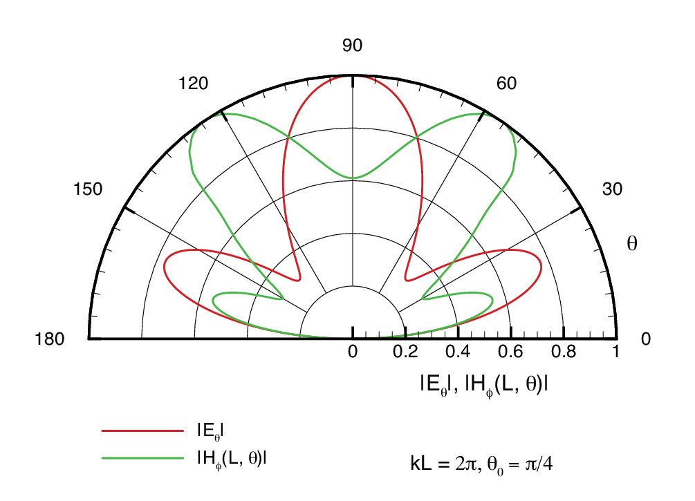
The E-plane variation of far-zone electric field $E_{\theta}$ and near-zone magnetic field $H_{\phi}(r=L,\theta)$ of the antenna with $kL=2\pi,\theta_{0}=\pi/4$ are shown in Fig. 5. Both fields are normalized with respect to their maximum fields. The far-zone pattern for an electrically small biconical antenna resembles that of short dipole. However, for the pattern shown in Fig. 5 for a radius of $L/\lambda=1$, a single-lobed broadside beam is observed for the biconical antenna. This is in contrast to a two wavelength long cylindrical dipole, which will have split beams [18].

Using the field expressions (18)-(20) and the identities (24), (25), the complex power flowing out of a sphere of radius $r>L$ can be shown to be

where $\Omega$ denotes the unit sphere. The real part of the complex power flow gives the power radiated, $P_{\rm rad}^{+}$, in the volume exterior to the antenna. The superscript ⁺ denotes that fields exterior to $r=L$ have been used in obtaining it. The normalized radiated power is

where the Wronskian for the spherical Riccati-Hankel function $W_{H}=\widehat{H}_{\ell}^{(2)\prime}(z)\widehat{H}^{(1)}_{\ell}(z)-\widehat{H}_{\ell}^{(1)\prime}(z)\widehat{H}_{\ell}^{(2)}(z)=-2j$ has been used in arriving at the result. The radiated power is seen to be independent of the radius $r$ as expected.

The radiated power could also be calculated using the field expressions (3), (4) interior to the sphere $r=L$. Utilizing (7), (9), and (27) gives

where the superscript ^- indicates that the fields in the region $r<L$ have been used. The operator $\Re(\cdot)$ denotes ‘real part’ of a quantity. Evidently, $P_{o}^{-}$ is also independent of the radius $r$. It is easy to verify that the quantities on the RHSs of (41) and (42) are identical to each other by following these sequential steps:

1. (i)

   Start from equation (31), multiply both sides of it by $-jc_{m}$ and sum over all $m=1,3,\ldots\infty$,

2. (ii)

   Take the real part of the resulting summation,

3. (iii)

   Utilize the symmetry relation $g_{m\ell}=g_{\ell m}$ and the Wronskian $W_{H}$ to arrive at the end result.

Consequently, we set $P_{\rm rad}^{+}=P_{\rm rad}^{-}=:P_{\rm rad}$ and $P_{o}^{+}=P_{o}^{-}=:P_{o}$. Irrespective of which fields are used in the computation of radiated power, it is seen that finding the mode coefficients $c_{\ell}$ in the exterior region is central.

References

- [1] S. A. Schelkunoff, “Principal and complementary waves in antennas,” Proc. IRE, vol. 34, pp. 23–32, 1946.
- [2] ——, Advanced Antenna Theory. New York, NY: John Wiley & Sons, Inc., 1952.
- [3] C. T. Tai, “On the theory of biconical antennas,” J. Applied Physics, vol. 19, pp. 1155–1159, December 1948.
- [4] R. E. Collin and F. J. Zucker, Antenna Theory, Pt. 1, ser. Inter-University Electronics Series. New York, NY: Mc-Graw-Hill Book Co., 1969, vol. 7.
- [5] C. T. Tai, Antenna Engineering Handbook. New York, NY: Mc-Graw-Hill Book Co., 1984, ch. Ch. 4: Dipoles and Monopoles.
- [6] C. H. Papas and R. W. P. King, “Input impedance of wide-angle conical antennas fed by a coaxial line,” Proc. IRE, vol. 37, pp. 1269–1271, 1949.
- [7] ——, “Radiation from wide-angle conical antennas fed by a coaxial line,” Proc. IRE, vol. 39, pp. 49–51, 1951.
- [8] R. M. Bevensee, Handbook of Conical Antennas and Scatterers. New York: Gordon and Breach, 1973.
- [9] P. E. Mayes and W. Gee, “Tunable, wide-angle conical monopole with selectable bandwidth,” in Proceedings of the 1995 Antenna Applications Symposium. Hanscom AFB, MA: Rome Laboratory, 1995, pp. 352–381.
- [10] S. N. Samaddar and E. L. Mokole, “Biconical antennas with unequal cone angles,” IEEE Trans. Antennas Propagat., vol. 46, no. 2, pp. 181–192, November 1998.
- [11] S. Z. Sapuan, A. Kazemipour, and M. Jenu, “Direct feed biconical anenna as a reference antenna,” in Proceedings of 2011 IEEE International RF and Micorwave Conference (RFM 2011), Seremban, Malaysia, 12-14 December 2011.
- [12] R. Janaswamy, “Biconical antenna: A wideband benchmark antenna for IEEE P2816,” in Proceedings of 2021 IEEE International Symposium on Antennas and Propagation and USNC-URSI Radio Science Meeting, Marina Bay Sands, Singapore, 4-10 December 2021, p. Paper # 1745.
- [13] A. D. Yaghjian and S. R. Best, “Impedance, bandwidth and Q of antennas,” IEEE Trans. Antennas Propagat., vol. 53, no. 4, pp. 1298–1324, April 2005.
- [14] J. S. McLean, “A re-examination of the fundamental limits on the radiation Q of electrically small antennas,” IEEE Trans. Antennas Propagat., vol. 44, no. 5, pp. 672–676, May 1996.
- [15] S. R. Best, “The Foster reactance theorem and quality factor for antennas,” IEEE Antennas Wireless Propagat. Lett., vol. 3, no. 1, pp. 306–309, 2004.
- [16] L. J. Chu, “Physical limitations of omni-directional antennas,” J. Applied Physics, vol. 19, pp. 1163–1175, December 1948.
- [17] M. Gustafsson and C. Sohl and G. Kristensson, “Physical limitations on antennas of arbitrary shape,” Proc. Royal. Soc. A, vol. 463, pp. 2589–2607, July 2007.
- [18] W. L. Stutzman and G. A. Thiele, Antenna Theory and Design, 3rd ed. Hoboken, NJ: John Wiley & Sons, Inc., 2013.
- [19] C. A. Balanis, Advanced Engineering Electromagnetics, 2nd ed. New York: John Wiley & Sons, Inc., 2012.
- [20] J. M. Jin, Theory and Computation of Electromagnetic Fields, 2nd ed. New York, NY: John Wiley & Sons, Inc., 2015.
- [21] R. Janaswamy, Engineering Electrodynamics: A collection of theorems, principles and field representations. Bristol, U.K.: Institute of Physics, December 2020.
- [22] S. A. Schelkunoff, Applied Mathematics for Engineers and Scientists. Princeton, NJ: Van Nostrand, 1965.
- [23] N. N. Lebedev, Special Functions and Their Applications. New York, NY: Dover Publications, 1972.
- [24] I. S. Gradshteyn and I. M. Ryzhik, Tables of Integrals, Series and Products, 7th ed. Academic Press, 2007.
- [25] B. Mrdakovic, “Personal communication,” Head of R&D, WIPL-D Commerical Software, May 26 2021.
- [26] M. Capek and L. Jelinek, “Comments on ‘Stored energy and radiation Q’,” IEEE Trans. Antennas Propagat., vol. 64, pp. 4575–4576, 2016.
- [27] C. J. Reddy, “Personal communication,” VP-Electromagnetics, Altair Feko Commerical Software, November 2021.
- [28] R. F. Harrington, “Effect of antenna size on gain, bandwidth and efficiency,” J. Res. Natl. Bur. Stds.-D, Radio Propagation, vol. 64D, no. 1, pp. 1–12, January-February 1960.
- [29] R. E. Collin and S. Rothschild, “Evaluation of antenna Q,” IEEE Trans. Antennas Propagat., vol. 12, pp. 23–27, January 1964.
- [30] R. L. Fante, “Quality factor of general ideal antennas,” IEEE Trans. Antennas Propagat., vol. AP-17, no. 2, pp. 151–155, March 1969.
- [31] M. Gustafsson and B. L. G. Jonsson, “Stored electromagnetic energy and antenna Q,” Progress in Electromagnetics Research, vol. 150, pp. 13–27, 2015.