Inflation Revisited and Dark Energy Corrections
Abstract
The vacuum model is known to generate a quasi-de Sitter evolution for inflation, using solely the slow-roll assumptions. Using standard reconstruction techniques, we demonstrate that the gravity which actually realizes the quasi-de Sitter evolution is not simply the model but a deformed model which contains extra terms in addition to the model. We analyze in detail the inflationary dynamics of the deformed model and we demonstrate that the predictions are quite close to the ones of the pure model, regardless the values of the free parameters. Basically the deformed model is also a single parameter inflationary model, exactly like the ordinary model. In contrast to the early-time era, where the deformed model is quite similar to the model, at late times, the phenomenological picture is different. The deformed model describes stronger gravity compared to the ordinary with an effectively smaller effective Planck mass. We propose the addition of an early dark energy term which does not affect at all the inflationary era, but takes over the control of the late-time dynamics at late times. We study in some detail the predicted dark energy era evolution, and we demonstrate that the dark energy corrected deformed model can describe a viable dark energy era, compatible with the Planck constraints on cosmological parameters. Furthermore the model is distinct from the -Cold-Dark-Matter model, but shows a qualitatively similar behavior.
pacs
04.50.Kd, 95.36.+x, 98.80.-k, 98.80.Cq,11.25.-wI Introduction
We are nearing the stage four epoch of Cosmic Microwave Background (CMB) experiments, and all the scientific research related to cosmology are focused on finding the -modes of inflation. In general, these curl modes of the CMB can be generated in two ways, firstly from the gravitational lensing conversion of -modes to -modes at small angular scales or large multipoles of the CMB, or by the tensor perturbations at low multipoles of the CMB or at large angular scales. The latter is the main focus of the stage-4 CMB experiments, such as CMB-S4 CMB-S4:2016ple and the Simons Observatory SimonsObservatory:2019qwx. In addition to these stage four CMB experiments, the scientific community of astrophysicists and cosmologists are eagerly anticipating the results of several other scientific experiments and space observatories, which may reveal the existence of primordial gravitational waves, among other things. Future collaborations and experiments like the Einstein Telescope Hild:2010id, the LISA Space-borne Laser Interferometer Space Antenna Baker:2019nia; Smith:2019wny the BBO Crowder:2005nr; Smith:2016jqs, DECIGO Seto:2001qf; Kawamura:2020pcg and finally the SKA (Square Kilometer Array) Pulsar Timing Arrays Bull:2018lat are eagerly expected from theoretical cosmologists and astrophysicists, since all the aforementioned collaborations will shed light to the most mysterious era of our Universe, the early-time post-Planck era. Indeed, inflation and reheating and even the early stages of the radiation domination era will possibly reveal their secrets via the primordial gravitational wave spectrum. In some sense, high energy physicists, theoretical cosmologists and theoretical astrophysicists will focus their interest on the CMB stage 4 experiments and on the space collaborations capturing primordial gravitational waves. The future of theoretical particle physics seems to be in the sky eventually.
In view of these future and nearing experiments, many theoretical models will be scrutinized and stress tests will verify their validity and the limits of their validity. Inflation inflation1; inflation2; inflation3; inflation4 is one of the most successful and elegant theoretical descriptions of the post-Planck early time, since it explains in a rigid way most of the shortcomings of the standard Big Bang cosmology. However, to date, no sign of the -mode polarization in the CMB has ever been observed, nor a sign of a stochastic gravitational wave background has ever been observed. It is conceivable that if a direct signal of -modes in the CMB is observed Kamionkowski:2015yta, or if a stochastic gravitational wave background is observed, this would signify directly that inflation indeed took place.
With all the upcoming experiments which are expected to stir up things in theoretical cosmology, many models of inflation might be in peril to become non-viable. In most cases, inflationary models rely on single scalar fields, minimally or non-minimally coupled. However, another promising approach which can realize a viable inflationary era without relying to scalar fields, or at least not relying solely on scalar fields, is modified gravity in its various forms reviews1; reviews2; reviews3; reviews4; reviews5; reviews6. There are many kinds of modified gravities that can successfully describe inflation, such as gravity Nojiri:2003ft; Capozziello:2005ku; Capozziello:2004vh; Capozziello:2018ddp; Hwang:2001pu; Cognola:2005de; Nojiri:2006gh; Song:2006ej; Capozziello:2008qc; Bean:2006up; Capozziello:2012ie; Faulkner:2006ub; Olmo:2006eh; Sawicki:2007tf; Faraoni:2007yn; Carloni:2007yv; Nojiri:2007as; Capozziello:2007ms; Deruelle:2007pt; Appleby:2008tv; Dunsby:2010wg; Odintsov:2020nwm; Odintsov:2019mlf; Odintsov:2019evb; Oikonomou:2020oex; Oikonomou:2020qah, Gauss-Bonnet gravity Nojiri:2005vv; Nojiri:2005jg; Lidsey:2003sj; Carter:2005fu; Cognola:2006eg; Leith:2007bu; Li:2007jm; Bamba:2010wfw; Odintsov:2020sqy; Kanti:2015dra; Oikonomou:2015qha; Kanti:2015pda; Oikonomou:2021kql and so on, and in some cases a unified description of the inflationary era with the dark energy era can also be described even with the same model, as in the pioneer work Nojiri:2003ft, see also Nojiri:2006gh; Nojiri:2007as; Appleby:2008tv; Odintsov:2019evb; Oikonomou:2020oex; Oikonomou:2020qah for later developments. In this work we shall consider deformations of gravity Starobinsky:1980te; Bezrukov:2007ep caused by demanding a quasi de Sitter evolution during the early-time era, the widely known in the literature as Starobinsky inflation. The reason for this is simple, it is known in the literature that if we solve the gravity equations of motion using the slow-roll conditions, one obtains a quasi-de Sitter evolution. However, in the converse way, if we demand a quasi-de Sitter evolution to be realized by vacuum gravity, by using standard reconstruction techniques, we will show that the resulting gravity contains the model, but there are also other terms in the final form of the quasi-de Sitter realizing gravity. We thoroughly investigate the effect of the extra terms in the inflationary Lagrangian, on the inflationary dynamics of the model, using only the slow-roll condition. As we show, the resulting model is nothing but a slight deformation of the model, the dynamics are very similar and almost identical. However, at late times, the extra terms might affect the dynamics significantly. Specifically, in the small curvature limit, which describes the late-time era, the effective Planck mass is effectively smaller compared to the early time era, thus in some sense, effectively gravity becomes stronger at late times. We also propose the addition of an early dark energy term in the full deformed Lagrangian, which does not affect at all the inflationary era, but strongly affects the late-time era. As we show, the dark energy deformed model provides a viable late-time phenomenology at late times, and serves as a viable deformation of the -Cold-Dark-Matter (CDM) model.
This paper is organized as follows: In section II we discuss the essential features of the quasi-de Sitter evolution and how can this evolution be realized by a vacuum gravity. We also calculate in the same section the form of the gravity and that the resulting form is a deformation of the model. In section III we study in detail the inflationary phenomenology of this model and discuss several limiting cases of the deformed model. In section IV we propose an early dark energy term which does not affect inflation at all, but does affect the late-time era significantly, and we show that the dark energy corrected deformed model can produce a viable dark energy era and mimic to some extent the CDM model. Finally, the conclusions follow in the end of the paper.
Before starting, let us mention that he geometric background which will be assumed, is that of a flat Friedmann-Robertson-Walker (FRW) background of the form,
| (1) |
where being as usual the scale factor. We shall also adopt the natural units physical system of units.
II Quasi-de Sitter Evolution and Realization from Gravity
The inflationary era is basically realized in general relativity by a de Sitter or a quasi-de Sitter evolution at least. It is quite difficult to capture the entire evolution of the Universe during the post-Planck era, however, we have phenomenological and theoretical hints on how the Universe evolves during the various cosmological eras. One hint is that during an accelerating era, the Universe must evolve for a large number of -foldings in a quasi-de Sitter way. We need to stress that this quasi-de Sitter era is a transient era and not a permanent state. The physics of the effective inflationary Lagrangian will stop the quasi-de Sitter era at some point and the Universe will enter the mysterious reheating era, in which the equation of state (EoS) will be described by radiation or some variant form in alternative kination scenarios. Here we shall focus on the quasi-de Sitter phase and we shall analyze in detail the physics of it. We shall reveal interesting features of the standard model, which elevate the role of the standard model to one of the most elegant descriptions of the early Universe, to date at least. To start off, consider the following quasi-de Sitter evolution,
| (2) |
where is basically the scale of inflation and has mass dimensions in natural units , is a parameter which deforms the de-Sitter to a quasi-de Sitter evolution, which plays an important role in the inflationary evolution, and is the time instance on which the quasi-de Sitter evolution commences. From Eq. (2) we easily obtain the scale factor of the quasi-de Sitter evolution, which is,
| (3) |
and the normalization factor can be taken be unity in order for the comoving scales to be identical with real physical scales during inflation, but we leave this as it is. Let us study the behavior of the quasi-de Sitter evolution (2) in order to further understand this evolution patch of our Universe and to better understand this inflationary evolution. In Fig. 1 we present the behavior of the scale factor as a function of the cosmic time (left plot) and the Hubble radius as a function of the cosmic time (right plot). As it can be seen, the scale factor grows exponentially for a sufficient amount of time, however the quasi-de Sitter patch of the Universe starts to drop after some point in time. It is clear that this time instance must be the one for which inflation ends. The Hubble radius accordingly drops until some point where it starts to grow again. Basically the point at which the Hubble radius reaches a minimum, basically indicates the end of the inflationary era.
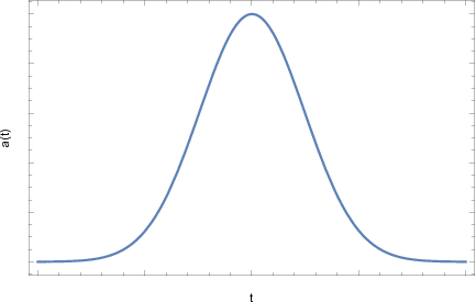
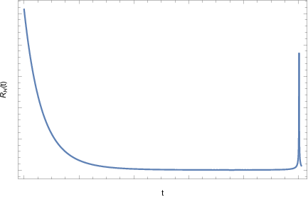
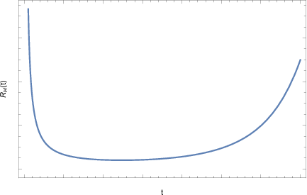
We can calculate analytically this point by finding the critical points of the Hubble radius upon solving , which yields,
| (4) |
and is basically the time instance for which . At this time instance the acceleration era ends, and the Universe starts to decelerate again. Remarkably, if one calculates, for the same scale factor the solution to the equation , one obtains the solution (4), and recall that the condition for which the first slow-roll index becomes of the order , namely, indicates the time instance for which inflation ends. This is a remarkable feature of the quasi-de Sitter evolution (2) which describes in an accurate way a smooth and phenomenologically appealing inflationary era, since the time instance for which inflation ends is exactly the time instance for which the Hubble radius starts to increase. This behavior should be obtained from any viable inflationary model and it describes an ideal and desirable inflationary evolution.
Let us now demonstrate how the quasi-de Sitter cosmology (2) can be realized by gravity. We consider a vacuum gravity theory with action,
| (5) |
with being and with denoting the reduced Planck mass. In the metric formalism, the field equations can be obtained by varying the gravitational action with respect to the metric tensor, so we obtain,
| (6) |
with . We can rewrite (6) as follows,
| (7) |
For the FRW metric (1), the field equations take the form,
| (8) | ||||
| (9) |
with , and , with being the Hubble rate and the Ricci scalar for the FRW metric is .
We can find which gravity can realize the quasi-de Sitter evolution (2) by using the reconstruction technique developed in Nojiri:2009kx, which is based on using the -foldings number instead of the cosmic time, defined in terms of the scale factor as,
| (10) |
In terms of , the Friedmann equation (8) is written as,
| (11) |
where the prime denotes differentiation with respect to the -foldings number. We introduce the function , and therefore the Ricci scalar reads,
| (12) |
and from this one can easily obtain the function . For the quasi-de Sitter evolution (2), we have,
| (13) |
Upon combining Eqs. (12) and (13), we get the -foldings number as a function of the Ricci scalar,
| (14) |
The Friedmann equation can be written in terms of the function as follows,
| (15) |
with and . By using Eq. (14), the Friedmann equation reads,
| (16) |
which can be solved and yields the gravity which can realize the quasi-de Sitter evolution (2), which is,
| (17) |
where and are integration constants. The standard coupling of the Einstein-Hilbert term can be obtained by choosing , so we have,
| (18) |
where the constant of integration has mass dimensions . As it can be seen, the gravity contains the standard model among other alternative terms. The standard gravity in the slow-roll approximation realizes the quasi-de Sitter evolution, and using the reconstruction technique, without assuming for the moment the slow-roll condition, we demonstrated that the quasi-de Sitter evolution is not realized by the model solely, but from the gravity of Eq. (18). In the next section, we shall analyze in detail the inflationary predictions of the model (18).
III Inflationary Phenomenology of the quasi-de Sitter Realizing Extended Gravity
We shall be interested in analyzing in some detail the inflationary phenomenology of the gravity appearing in Eq. (18) which is basically a deformation of the model, under the assumption of slow-roll dynamics,
| (19) |
The slow-roll indices, namely ,, , , basically quantify the inflationary era dynamics and for the case of gravity, these read Hwang:2005hb; reviews1,
| (20) |
Assuming that , and the observational indices of inflation, namely the spectral index of the primordial scalar perturbations, the tensor-to-scalar ratio and the spectral index of the tensor perturbations, expressed in terms of the slow-roll indices are reviews1; Hwang:2005hb; Kaiser:1994vs,
| (21) |
From the Raychaudhuri equation, in the case of vacuum gravity we get the following relation,
| (22) |
Now with regard to the slow-roll index , we shall express it in terms of the first slow-roll index. After some algebra we have,
| (23) |
and by using the slow-roll assumption, is approximately equal to,
| (24) |
where we used the slow-roll approximation condition . Then by combining Eqs. (24) and (23) after some algebra we obtain,
| (25) |
and since is,
| (26) |
we obtain the final expression for the slow-roll index which is,
| (27) |
Let us apply the formalism for the specific deformation of the model in Eq. (18). For convenience, let us introduce the parameter , so that is written in terms of it,
| (28) |
The parameter basically quantifies the deformation of the model (18) compared to the model.
Let us calculate in detail the slow-roll indices for the case at hand, starting with which is,
| (29) |
and can easily be found from Eq. (22). For it suffices to calculate the parameter defined below Eq. (27), which reads,
| (30) |
where is defined as,
| (31) | ||||
By solving we may obtain the time instance that inflation ends, which is , and by solving the equation for the quasi-de Sitter evolution (2) with respect to , we may obtain the latter which is the time instance at the first horizon crossing. At this time instance one needs to evaluate the slow-roll indices and the corresponding observational indices. The first horizon crossing time instance reads, . Evaluating the spectral index of scalar perturbations at for -foldings we get the following approximate expression,
| (32) | ||||
where and are defined as follows,
| (33) | ||||
and by simply assuming that and keeping the leading order terms, we have, regardless the values of the free parameters , , which is quite close to the value which corresponds to the pure model. Now, with regard to the tensor-to-scalar ratio, for -foldings and for this reads,
| (34) |
so by keeping the dominant terms we get at leading order , and this value is obtained irrespective of the values of the free parameters and and it is quite close to the one corresponding to the pure model which is . Accordingly the tensor spectral index for the model at hand reads,
| (35) |
hence by keeping the dominant terms we have approximately irrespective of the values of the free parameters. Thus overall, the pure model and the deformed model (18) have quite similar phenomenology during inflation. This can also be seen in Fig. 2 where we present the combined -plot for the deformed model confronted with the latest Planck likelihood curves for chosen in the range . As it can be seen, the model has quite elegant viability characteristics comparable and almost identical with the standard model.

So far we have not defined the integration constant which is arbitrary. However, at this point we shall fix it by using the asymptotic limit of the deformed gravity (18) at late times, thus for , in which limit the deformed reads,
| (36) | ||||
and we can fix by fixing the asymptotical limit (36) to have zero effective cosmological constant. Thus if we demand for late-time reasoning the last term to vanish, the constant must be chosen as so the asymptotic form of the gravity (36) becomes,
| (37) |
It is notable that the late-time era for the model at hand is described by a rescaled Einstein-Hilbert term. This is an effective theory with a weaker gravity compared to the Einstein-Hilbert term. Basically, the leading order Einstein-Hilbert term is a rescaled Einstein-Hilbert term with a smaller effective Planck mass compared to the simple Einstein-Hilbert term . In the next section, we shall propose an effective correction term which has no effect during the inflationary era, but when it is combined with the gravity (37), results to an early dark energy evolution at late times, and more importantly, it results to a viable dark energy era at present time.
IV Late-time Behavior and Proposal for Dark Energy Correction Terms
In this section we shall investigate the late-time perspectives of the deformed model of Eq. (18) by also adding a correction term of the form where is the present time cosmological constant, eV2 and is the parameter appearing in the deformed model, which in for strictly phenomenological reasons related to the amplitude of the scalar perturbations in the Einstein frame version of the pure model, must be chosen Appleby:2009uf, hence for , is eV. At late-time thus, by using the expansion (37), and by adding the correction term , the late-time gravity reads,
| (38) | ||||
Note that the unified description scheme of inflation with dark energy in the context of gravity, was first proposed in Nojiri:2003ft and extended to a number of models in the review reviews4. Also, one can consider such unification of deformed inflation with dark energy, using other gravity terms which do not affect inflation, but produce a viable dark energy era, such as subdominant power-law terms. A couple of comments prior to continuing to the phenomenological analysis of the model at hand. Firstly, the correction term has no effect during early times, when the curvature takes large values. Thus it is essentially an early dark energy term which is inactive at early times but takes over the control of the dynamics of the model at late times. This issue is important and at this point we shall analyze it in detail. One question is, why did not the early dark energy correction term did not appear from the first place in the gravity which realizes the quasi-de Sitter evolution, namely in Eq. (18). The answer is simple, the gravity in Eq. (18) is the gravity which realizes the quasi-de Sitter patch of the Universe at early times. Hence it is a leading order behavior of the full underlying gravity, which is unknown to us. Hence in general, there might be many other subdominant terms during the quasi-de Sitter era of the Universe, which are unknown to us. One of these possible terms could be the one we introduced , which is truly subdominant during inflation, as we now evince. It is a big problem for scientists to know the exact form of gravity which may control the full evolution history of our Universe, and the problem relies to our inability to find a totally unified evolution of the Universe in terms of a unique Hubble rate. Instead of that, we have only clues for four distinct evolutionary era of our Universe, the inflationary era, usually realized successfully by a quasi-de Sitter evolution, the radiation domination era followed by a matter domination era which lastly is followed by a dark energy era. Thus we basically have patches of evolution for which we know some things and not a unified evolutionary behavior in terms of a unique Hubble rate. An example of a unified scalar factor describing all the eras would be,
| (39) |
where denotes the scale factor at the beginning of the inflationary era, denotes the scale factor at the end of inflation and at the start of the radiation domination era, denotes the scale factor at the end of the radiation domination era and at the beginning of the dark matter domination era, and finally denotes the scale factor at the end of the matter domination era and at the beginning of the dark energy era. As it is apparent from Eq. (39), it is impossible to find using the reconstruction technique we introduced in the previous section which gravity realizes such an evolution, at least in an analytic way. It is simply an inevitable task. However what we certainly do is to find which underlying gravity may realize each evolutionary patch separately. Thus in the previous section we showed that the dominant gravity form which is responsible for the realization of the quasi-de Sitter patch, namely the first term in Eq. (39), is given by the gravity appearing in Eq. (18). It is however highly possible that many subdominant terms appear in the effective inflationary Lagrangian, which are responsible for the realization of one of the three last terms in Eq. (39). An example of this sort is played by the early dark energy term which we added by hand, namely . This term is totally ignorable during inflation, and is actually activated only at late times, and specifically for the redshift range . Let us show that this term is indeed inactive during inflation. As we mentioned in the beginning of this section, for the dark energy era analysis we shall take eV2 and eV and also the scale of inflation is GeV. For these values, and during inflation, in which case , the term is of the order eV, while the term eV and the early dark energy term eV. Thus it is apparent that the early dark energy term is highly subdominant during inflation and therefore it does not affect at all the dynamics during inflation. However as we evince in this section, it affects significantly the late time dynamics of the cosmological system.
Furthermore, the model (38) has effectively a larger effective Newton gravitational constant, or a smaller effective Planck mass, compared to Einstein-Hilbert gravity. This is due to the fact that the deformed gravity of Eq. (18) asymptotically for small curvature values at linear order in behaves as,
| (40) |
and the second term is basically a negative term which effectively reduces the effective Planck mass or equivalently it increases the strength of gravity at late times. Hence for the model at hand, the late-time era gravity is stronger at linear order, compared to the standard Einstein-Hilbert term. Now we shall analyze in detail the late-time dynamics of the model (38), emphasizing in studying quantities of cosmological interest which we now discuss. We shall assume that along with the gravity model (38), radiation and cold dark matter fluids are present, which were neglected during the early time era. For the gravity in the presence of matter fluids, the field equations can be written in the Einstein-Hilbert form in the following way,
| (41) | ||||
where the total energy density is equal to , and and are the matter and radiation fluids energy densities respectively. Also the dark energy density is the geometric contribution of the gravity fluid, which essentially will control the late-time dynamics, and it is defined as follows,
| (42) |
The corresponding total pressure , and the dark energy pressure is defined as,
| (43) |
In order to study the late-time dynamics of the model (38), we shall introduce some statefinder quantities in terms of the redshift, which we shall use as a dynamical parameter. This will facilitate our late-time study. Firstly, the redshift parameter is,
| (44) |
and we assumed that present time scale factor, at , is equal to unity. In this way, physical wavelengths and comoving wavelengths coincide at late times. We introduce the statefinder function Hu:2007nk; Bamba:2012qi; Odintsov:2020vjb; Odintsov:2020nwm; Odintsov:2020qyw; reviews1,
| (45) |
where is the energy density of cold dark matter at present time. Being a statefinder quantity, quantifies the effects of dark energy at late times, and it is certainly different from zero, when geometric terms affect the late-time dynamics. This can be true in two cases, firstly when a cosmological constant is directly present in the effective Lagrangian, or even when geometric terms of a higher order gravity are present in the Lagrangian. If is zero, this case simply describes the Einstein-Hilbert FRW cosmology without a cosmological constant. Using Eq. (41), we can write the function as follows,
| (46) |
where recall that and also we introduced defined as , and denotes the radiation energy density at present time. Also the parameter is defined as eV2, and we used the Planck 2018 constraints on the cosmological parameters, which indicate that eV. Hence the statefinder quantity indicates deviations from the standard CDM model, in which case it would simply be a constant. In the case of gravity, the function indicates the dynamical dark energy character of the late-time behavior. Rewriting the Friedmann equations in terms of the function and using the redshift parameter as a dynamical parameter we get,
| (47) |
where the dimensionless functions , and are defined as,
| (48) | ||||
where we defined and , while . We shall solve numerically the differential equation (47) focusing on the late-time redshift interval , by using following set of initial conditions
| (49) |
which are well motivated and justified by the late moments of the matter domination era Hu:2007nk; Bamba:2012qi; Odintsov:2020vjb; Odintsov:2020nwm; Odintsov:2020qyw; reviews1. For our analysis we shall focus on several physical cosmology quantities of interest, which we shall rewrite in terms of the statefinder function . A vital quantity is the curvature, which in terms of it is written as,
| (50) |
Accordingly, the dark energy density parameter is written as,
| (51) |
and this quantity is quite important since its present day value is accurately constrained by the Planck 2018 constraints Planck:2018vyg. The same applies for the dark energy EoS parameter , which is,
| (52) |
and a parameter which is quite important for the overall behavior of the model is the total EoS parameter which reads,
| (53) |
With regard to popular statefinder quantities, we shall choose the deceleration parameter , which in terms of the redshift is defined as follows,
| (54) |
In the following we shall compare the dark energy corrected model deformed model (38) with the Planck data at present time, or the CDM model where it is possible, with the CDM model Hubble rate in terms of the redshift being defined as follows,
| (55) |
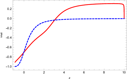
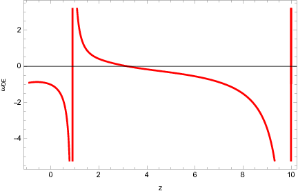
where is the value of the Hubble rate at present day. Moreover, and Planck:2018vyg, while , and recall is defined below Eq. (46). Let us present now the results of our numerical analysis in some detail. In Fig. 3 we present the behavior of the function (left plot), the total EoS parameter (right plot) and the dark energy EoS parameter (bottom plot) as functions of the redshift. The behavior of indicates firstly that the model deviates from the CDM model and it basically describes an early dark energy era. The same conclusion can be obtained by looking at the plot of the dark energy EoS parameter, where two steep acceleration eras appear to have occurred in the past. The total EoS parameter in the right plot of Fig. 3 contains the behavior of the total EoS parameter for the deformed model (red curve) compared with the CDM plot (blue curve). One thing is apparent for sure, qualitatively the deformed model behaves as the CDM model, however it seems that the deformed model is a deformation of the CDM model and there are clear distinctions between the two models.
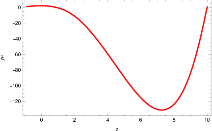
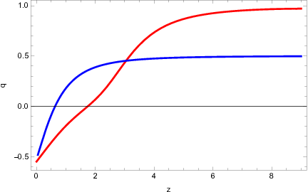
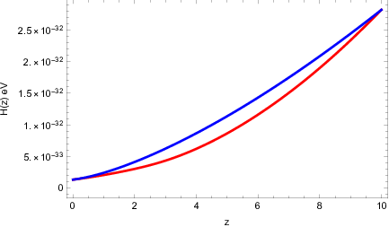
The same conclusion can be reached by looking Fig. 4 where we plot the deceleration parameter for the deformed model (red curves) and for the CDM model (blue curves). A notable feature for the deformed model is that the transition from deceleration to acceleration occurs earlier compared to the CDM model. Finally, in Fig. 5 we plot the Hubble rate for for the deformed model (red curves) and for the CDM model (blue curves). In general the CDM model has larger values for the Hubble rate during the whole range however, at present day the deformed model has slightly elevated value for the Hubble rate compared to the CDM model. In Table 1 we gather some characteristic values for the several physical cosmology quantities of interest. As it can be seen, the dark energy deformed model is quite compatible with the latest Planck constraints on cosmological parameters Planck:2018vyg. One of the most important parameters is the dark energy EoS parameter, which for the deformed model it reads which lies within the viability limits of the Planck constraint . A notable feature, mostly absent in the majority of gravity models is the fact that the dark energy era at present day is slightly phantom. Another important quantity is the dark energy density parameter, which for the deformed model reads, , and the Planck constraints on this are . Also in Table 1 it can be seen that the Hubble rate value at present day is slightly elevated for the deformed model in comparison to the CDM model, and it is contrasted with the overall behavior of the two models for intermediate redshifts.
| Cosmological Parameter | Deformed Gravity Value | Base CDM or Planck 2018 Value |
| 0.684831 | ||
| -1.02159 | ||
| -0.54938 | -0.535 | |
| in eV |
Overall, the dark energy corrected deformed model provides a viable description for the dark energy era, which mimics qualitatively the evolution of the CDM model, without overlaps between the two models though. Thus with the extra dark energy correction term, which during inflation does not affect at all the dynamics, but takes control over the dynamics of the model at late times, it is possible to provide a unified description of the inflationary era and the dark energy era with the same gravity model.
V Conclusions
In this work we pointed out that a quasi-de Sitter evolution in gravity is not solely realized by the vacuum model, as it is widely known in the literature, but from a deformed gravity, containing the model. By using a standard reconstruction technique, we calculated the exact form of the gravity which generates an exact quasi-de Sitter evolution. For the gravity we found, we calculated in detail the slow-roll indices and the observational indices of inflation, focusing on the spectral index of the primordial scalar and tensor perturbations, and the tensor-to-scalar ratio. As we demonstrated, the resulting model generates and inflationary evolution which is quantitatively similar to the model. The deformed model which generates the exact quasi-de Sitter evolution, at late-times yields an interesting characteristic, a stronger gravity in terms of the effective Newton’s constant at late times, or equivalently a smaller effective Planck mass at late times. We introduced an effective early dark energy correction term, which although did not affect the inflationary era, it affects the late-time evolution. Particularly, the dark energy era predicted by the deformed model we found is a deformed version of the CDM model, which is viable when confronted with the Planck 2018 data at present day, concerning the dark energy EoS and density parameters. Thus with this work, we revealed a hidden aspect of an inflationary quasi-de Sitter evolution in the context of gravity and we showed that there are effective correction terms to the standard model, which although they slightly affect the early time era, these may affect significantly the late-time era. The importance of the quasi-de Sitter evolution compels to perform further realizations of this important evolution patch of the Universe in other modified gravity frameworks, such as pure extended Gauss-Bonnet gravity Oikonomou:2015qha or even Einstein-Gauss-Bonnet gravity Koh:2014bka; Odintsov:2020sqy, or extensions of these theories, like Horndeski theories Bayarsaikhan:2020jww. We hope to address these issues in future works.
Acknowledgments
This work was supported by MINECO (Spain), project PID2019-104397GB-I00 (S.D.O).
References
- (1) K. N. Abazajian et al. [CMB-S4], [arXiv:1610.02743 [astro-ph.CO]].
- (2) M. H. Abitbol et al. [Simons Observatory], Bull. Am. Astron. Soc. 51 (2019), 147 [arXiv:1907.08284 [astro-ph.IM]].
- (3) S. Hild, M. Abernathy, F. Acernese, P. Amaro-Seoane, N. Andersson, K. Arun, F. Barone, B. Barr, M. Barsuglia and M. Beker, et al. Class. Quant. Grav. 28 (2011), 094013 doi:10.1088/0264-9381/28/9/094013 [arXiv:1012.0908 [gr-qc]].
- (4) J. Baker, J. Bellovary, P. L. Bender, E. Berti, R. Caldwell, J. Camp, J. W. Conklin, N. Cornish, C. Cutler and R. DeRosa, et al. [arXiv:1907.06482 [astro-ph.IM]].
- (5) T. L. Smith and R. Caldwell, Phys. Rev. D 100 (2019) no.10, 104055 doi:10.1103/PhysRevD.100.104055 [arXiv:1908.00546 [astro-ph.CO]].
- (6) J. Crowder and N. J. Cornish, Phys. Rev. D 72 (2005), 083005 doi:10.1103/PhysRevD.72.083005 [arXiv:gr-qc/0506015 [gr-qc]].
- (7) T. L. Smith and R. Caldwell, Phys. Rev. D 95 (2017) no.4, 044036 doi:10.1103/PhysRevD.95.044036 [arXiv:1609.05901 [gr-qc]].
- (8) N. Seto, S. Kawamura and T. Nakamura, Phys. Rev. Lett. 87 (2001), 221103 doi:10.1103/PhysRevLett.87.221103 [arXiv:astro-ph/0108011 [astro-ph]].
- (9) S. Kawamura, M. Ando, N. Seto, S. Sato, M. Musha, I. Kawano, J. Yokoyama, T. Tanaka, K. Ioka and T. Akutsu, et al. [arXiv:2006.13545 [gr-qc]].
- (10) A. Weltman, P. Bull, S. Camera, K. Kelley, H. Padmanabhan, J. Pritchard, A. Raccanelli, S. Riemer-Sørensen, L. Shao and S. Andrianomena, et al. Publ. Astron. Soc. Austral. 37 (2020), e002 doi:10.1017/pasa.2019.42 [arXiv:1810.02680 [astro-ph.CO]].
- (11) A. D. Linde, Lect. Notes Phys. 738 (2008) 1 [arXiv:0705.0164 [hep-th]].
- (12) D. S. Gorbunov and V. A. Rubakov, “Introduction to the theory of the early universe: Cosmological perturbations and inflationary theory,” Hackensack, USA: World Scientific (2011) 489 p;
- (13) A. Linde, arXiv:1402.0526 [hep-th];
- (14) D. H. Lyth and A. Riotto, Phys. Rept. 314 (1999) 1 [hep-ph/9807278].
- (15) M. Kamionkowski and E. D. Kovetz, Ann. Rev. Astron. Astrophys. 54 (2016) 227 doi:10.1146/annurev-astro-081915-023433 [arXiv:1510.06042 [astro-ph.CO]].
- (16) S. Nojiri, S. D. Odintsov and V. K. Oikonomou, Phys. Rept. 692 (2017) 1 [arXiv:1705.11098 [gr-qc]].
- (17)
S. Capozziello, M. De Laurentis,
Phys. Rept. 509, 167 (2011);
V. Faraoni and S. Capozziello, Fundam. Theor. Phys. 170 (2010). - (18) S. Nojiri, S.D. Odintsov, eConf C0602061, 06 (2006) [Int. J. Geom. Meth. Mod. Phys. 4, 115 (2007)].
- (19) S. Nojiri, S.D. Odintsov, Phys. Rept. 505, 59 (2011);
- (20) A. de la Cruz-Dombriz and D. Saez-Gomez, Entropy 14 (2012) 1717 [arXiv:1207.2663 [gr-qc]].
- (21) G. J. Olmo, Int. J. Mod. Phys. D 20 (2011) 413 [arXiv:1101.3864 [gr-qc]].
- (22) S. Nojiri and S. D. Odintsov, Phys. Rev. D 68 (2003), 123512 doi:10.1103/PhysRevD.68.123512 [arXiv:hep-th/0307288 [hep-th]].
- (23) S. Capozziello, V. F. Cardone and A. Troisi, Phys. Rev. D 71 (2005), 043503 doi:10.1103/PhysRevD.71.043503 [arXiv:astro-ph/0501426 [astro-ph]].
- (24) S. Capozziello, C. A. Mantica and L. G. Molinari, Int. J. Geom. Meth. Mod. Phys. 16 (2018) no.01, 1950008 doi:10.1142/S0219887819500087 [arXiv:1810.03204 [gr-qc]].
- (25) S. Capozziello, V. F. Cardone and M. Francaviglia, Gen. Rel. Grav. 38 (2006), 711-734 doi:10.1007/s10714-006-0261-x [arXiv:astro-ph/0410135 [astro-ph]].
- (26) J. c. Hwang and H. Noh, Phys. Lett. B 506 (2001), 13-19 doi:10.1016/S0370-2693(01)00404-X [arXiv:astro-ph/0102423 [astro-ph]].
- (27) G. Cognola, E. Elizalde, S. Nojiri, S. D. Odintsov and S. Zerbini, JCAP 02 (2005), 010 doi:10.1088/1475-7516/2005/02/010 [arXiv:hep-th/0501096 [hep-th]].
- (28) S. Nojiri and S. D. Odintsov, Phys. Rev. D 74 (2006), 086005 doi:10.1103/PhysRevD.74.086005 [arXiv:hep-th/0608008 [hep-th]].
- (29) Y. S. Song, W. Hu and I. Sawicki, Phys. Rev. D 75 (2007), 044004 doi:10.1103/PhysRevD.75.044004 [arXiv:astro-ph/0610532 [astro-ph]].
- (30) S. Capozziello, V. F. Cardone and V. Salzano, Phys. Rev. D 78 (2008), 063504 doi:10.1103/PhysRevD.78.063504 [arXiv:0802.1583 [astro-ph]].
- (31) R. Bean, D. Bernat, L. Pogosian, A. Silvestri and M. Trodden, Phys. Rev. D 75 (2007), 064020 doi:10.1103/PhysRevD.75.064020 [arXiv:astro-ph/0611321 [astro-ph]].
- (32) S. Capozziello and M. De Laurentis, Annalen Phys. 524 (2012), 545-578 doi:10.1002/andp.201200109
- (33) T. Faulkner, M. Tegmark, E. F. Bunn and Y. Mao, Phys. Rev. D 76 (2007), 063505 doi:10.1103/PhysRevD.76.063505 [arXiv:astro-ph/0612569 [astro-ph]].
- (34) G. J. Olmo, Phys. Rev. D 75 (2007), 023511 doi:10.1103/PhysRevD.75.023511 [arXiv:gr-qc/0612047 [gr-qc]].
- (35) I. Sawicki and W. Hu, Phys. Rev. D 75 (2007), 127502 doi:10.1103/PhysRevD.75.127502 [arXiv:astro-ph/0702278 [astro-ph]].
- (36) V. Faraoni, Phys. Rev. D 75 (2007), 067302 doi:10.1103/PhysRevD.75.067302 [arXiv:gr-qc/0703044 [gr-qc]].
- (37) S. Carloni, P. K. S. Dunsby and A. Troisi, Phys. Rev. D 77 (2008), 024024 doi:10.1103/PhysRevD.77.024024 [arXiv:0707.0106 [gr-qc]].
- (38) S. Nojiri and S. D. Odintsov, Phys. Lett. B 657 (2007), 238-245 doi:10.1016/j.physletb.2007.10.027 [arXiv:0707.1941 [hep-th]].
- (39) S. Capozziello, A. Stabile and A. Troisi, Phys. Rev. D 76 (2007), 104019 doi:10.1103/PhysRevD.76.104019 [arXiv:0708.0723 [gr-qc]].
- (40) N. Deruelle, M. Sasaki and Y. Sendouda, Prog. Theor. Phys. 119 (2008), 237-251 doi:10.1143/PTP.119.237 [arXiv:0711.1150 [gr-qc]].
- (41) S. A. Appleby and R. A. Battye, JCAP 05 (2008), 019 doi:10.1088/1475-7516/2008/05/019 [arXiv:0803.1081 [astro-ph]].
- (42) P. K. S. Dunsby, E. Elizalde, R. Goswami, S. Odintsov and D. S. Gomez, Phys. Rev. D 82 (2010), 023519 doi:10.1103/PhysRevD.82.023519 [arXiv:1005.2205 [gr-qc]].
- (43) S. D. Odintsov and V. K. Oikonomou, Phys. Rev. D 101 (2020) no.4, 044009 doi:10.1103/PhysRevD.101.044009 [arXiv:2001.06830 [gr-qc]].
- (44) S. D. Odintsov and V. K. Oikonomou, Phys. Rev. D 99 (2019) no.6, 064049 doi:10.1103/PhysRevD.99.064049 [arXiv:1901.05363 [gr-qc]].
- (45) S. D. Odintsov and V. K. Oikonomou, Phys. Rev. D 99 (2019) no.10, 104070 doi:10.1103/PhysRevD.99.104070 [arXiv:1905.03496 [gr-qc]].
- (46) V. K. Oikonomou, Phys. Rev. D 103 (2021) no.12, 124028 doi:10.1103/PhysRevD.103.124028 [arXiv:2012.01312 [gr-qc]].
- (47) V. K. Oikonomou, Phys. Rev. D 103 (2021) no.4, 044036 doi:10.1103/PhysRevD.103.044036 [arXiv:2012.00586 [astro-ph.CO]].
- (48) S. Nojiri, S. D. Odintsov and M. Sasaki, Phys. Rev. D 71 (2005), 123509 doi:10.1103/PhysRevD.71.123509 [arXiv:hep-th/0504052 [hep-th]].
- (49) S. Nojiri and S. D. Odintsov, Phys. Lett. B 631 (2005), 1-6 doi:10.1016/j.physletb.2005.10.010 [arXiv:hep-th/0508049 [hep-th]].
- (50) J. E. Lidsey and N. J. Nunes, Phys. Rev. D 67 (2003), 103510 doi:10.1103/PhysRevD.67.103510 [arXiv:astro-ph/0303168 [astro-ph]].
- (51) B. M. N. Carter and I. P. Neupane, JCAP 06 (2006), 004 doi:10.1088/1475-7516/2006/06/004 [arXiv:hep-th/0512262 [hep-th]].
- (52) G. Cognola, E. Elizalde, S. Nojiri, S. D. Odintsov and S. Zerbini, Phys. Rev. D 73 (2006), 084007 doi:10.1103/PhysRevD.73.084007 [arXiv:hep-th/0601008 [hep-th]].
- (53) B. M. Leith and I. P. Neupane, JCAP 05 (2007), 019 doi:10.1088/1475-7516/2007/05/019 [arXiv:hep-th/0702002 [hep-th]].
- (54) B. Li, J. D. Barrow and D. F. Mota, Phys. Rev. D 76 (2007), 044027 doi:10.1103/PhysRevD.76.044027 [arXiv:0705.3795 [gr-qc]].
- (55) K. Bamba, S. D. Odintsov, L. Sebastiani and S. Zerbini, Eur. Phys. J. C 67 (2010), 295-310 doi:10.1140/epjc/s10052-010-1292-8 [arXiv:0911.4390 [hep-th]].
- (56) S. D. Odintsov, V. K. Oikonomou and F. P. Fronimos, Nucl. Phys. B 958 (2020), 115135 doi:10.1016/j.nuclphysb.2020.115135 [arXiv:2003.13724 [gr-qc]].
- (57) P. Kanti, R. Gannouji and N. Dadhich, Phys. Rev. D 92 (2015) no.8, 083524 doi:10.1103/PhysRevD.92.083524 [arXiv:1506.04667 [hep-th]].
- (58) V. K. Oikonomou, Phys. Rev. D 92 (2015) no.12, 124027 doi:10.1103/PhysRevD.92.124027 [arXiv:1509.05827 [gr-qc]].
- (59) P. Kanti, R. Gannouji and N. Dadhich, Phys. Rev. D 92 (2015) no.4, 041302 doi:10.1103/PhysRevD.92.041302 [arXiv:1503.01579 [hep-th]].
- (60) V. K. Oikonomou, Class. Quant. Grav. 38 (2021) no.19, 195025 doi:10.1088/1361-6382/ac2168 [arXiv:2108.10460 [gr-qc]].
- (61) A. A. Starobinsky, Phys. Lett. B 91 (1980), 99-102 doi:10.1016/0370-2693(80)90670-X
- (62) F. L. Bezrukov and M. Shaposhnikov, Phys. Lett. B 659 (2008), 703-706 doi:10.1016/j.physletb.2007.11.072 [arXiv:0710.3755 [hep-th]].
- (63) S. Nojiri, S. D. Odintsov and D. Saez-Gomez, Phys. Lett. B 681 (2009), 74-80 doi:10.1016/j.physletb.2009.09.045 [arXiv:0908.1269 [hep-th]].
- (64) J. c. Hwang and H. Noh, Phys. Rev. D 71 (2005), 063536 doi:10.1103/PhysRevD.71.063536 [arXiv:gr-qc/0412126 [gr-qc]].
- (65) D. I. Kaiser, Phys. Rev. D 52 (1995), 4295-4306 doi:10.1103/PhysRevD.52.4295 [arXiv:astro-ph/9408044 [astro-ph]].
- (66) S. A. Appleby, R. A. Battye and A. A. Starobinsky, JCAP 06 (2010), 005 doi:10.1088/1475-7516/2010/06/005 [arXiv:0909.1737 [astro-ph.CO]].
- (67) W. Hu and I. Sawicki, Phys. Rev. D 76 (2007), 064004 doi:10.1103/PhysRevD.76.064004 [arXiv:0705.1158 [astro-ph]].
- (68) K. Bamba, A. Lopez-Revelles, R. Myrzakulov, S. D. Odintsov and L. Sebastiani, Class. Quant. Grav. 30 (2013), 015008 doi:10.1088/0264-9381/30/1/015008 [arXiv:1207.1009 [gr-qc]].
- (69) S. D. Odintsov, V. K. Oikonomou, F. P. Fronimos and K. V. Fasoulakos, Phys. Rev. D 102 (2020) no.10, 104042 doi:10.1103/PhysRevD.102.104042 [arXiv:2010.13580 [gr-qc]].
- (70) S. D. Odintsov, V. K. Oikonomou and F. P. Fronimos, Phys. Dark Univ. 29 (2020), 100563 doi:10.1016/j.dark.2020.100563 [arXiv:2004.08884 [gr-qc]].
- (71) N. Aghanim et al. [Planck], Astron. Astrophys. 641 (2020), A6 [erratum: Astron. Astrophys. 652 (2021), C4] doi:10.1051/0004-6361/201833910 [arXiv:1807.06209 [astro-ph.CO]].
- (72) V. K. Oikonomou, Phys. Rev. D 92 (2015) no.12, 124027 doi:10.1103/PhysRevD.92.124027 [arXiv:1509.05827 [gr-qc]].
- (73) S. Koh, B. H. Lee, W. Lee and G. Tumurtushaa, Phys. Rev. D 90 (2014) no.6, 063527 doi:10.1103/PhysRevD.90.063527 [arXiv:1404.6096 [gr-qc]].
- (74) S. D. Odintsov, V. K. Oikonomou and F. P. Fronimos, Nucl. Phys. B 958 (2020), 115135 doi:10.1016/j.nuclphysb.2020.115135 [arXiv:2003.13724 [gr-qc]].
- (75) B. Bayarsaikhan, S. Koh, E. Tsedenbaljir and G. Tumurtushaa, JCAP 11 (2020), 057 doi:10.1088/1475-7516/2020/11/057 [arXiv:2005.11171 [gr-qc]].