Impact of Massive Binary Star and Cosmic Evolution on Gravitational Wave Observations II: Double Compact Object Rates and Properties2021Impact of Massive Binary Star and Cosmic Evolution on Gravitational Wave Observations II: Double Compact Object Rates and Properties–13
Abstract
Making the most of the rapidly increasing population of gravitational-wave detections of BH (BH) and NS (NS) mergers requires comparing observations with population synthesis predictions. In this work we investigate the combined impact from the key uncertainties in population synthesis modelling of the isolated binary evolution channel: the physical processes in massive binary-star evolution and the star formation history as a function of metallicity, , and redshift , . Considering these uncertainties we create different publicly available model realizations and calculate the rate and distribution characteristics of detectable BHBH, BHNS, and NSNS mergers. We find that our stellar evolution and variations can impact the predicted intrinsic and detectable merger rates by factors –. We find that BHBH rates are dominantly impacted by variations, NSNS rates by stellar evolution variations and BHNS rates by both. We then consider the combined impact from all uncertainties considered in this work on the detectable mass distribution shapes (chirp mass, individual masses and mass ratio). We find that the BHNS mass distributions are predominantly impacted by massive binary-star evolution changes. For BHBH and NSNS we find that both uncertainties are important. We also find that the shape of the delay time and birth metallicity distributions are typically dominated by the choice of for BHBH, BHNS and NSNS. We identify several examples of robust features in the mass distributions predicted by all models, such that we expect more than 95 percent of BHBH detections to contain a BH and have mass ratios . Our work demonstrates that it is essential to consider a wide range of allowed models to study double compact object merger rates and properties. Conversely, larger observed samples could allow us to decipher currently unconstrained stages of stellar and binary evolution.
Keywords:
(transients:) black hole - neutron star mergers – gravitational waves – stars: evolution1 Introduction
The population of detected GW (GW) events from BHBH (BHBH), BHNS (BHNS) and NSNS (NSNS) mergers is rapidly increasing (Abbott et al. 2019; Abbott et al. 2020a; Abbott et al. 2021a; The LIGO Scientific Collaboration et al. 2021b). These mergers carry unique information about the properties of BH and NS (such as their masses and spins), which in turn probes the formation, lives, and explosive deaths of massive stars throughout cosmic history (Abbott et al. 2021b; The LIGO Scientific Collaboration et al. 2021c, e.g.). To extract information from these DCO (DCO) detections requires comparing their observed properties, to theoretically simulated populations modelling their formation pathways.
A variety of formation channels for DCO mergers have been proposed (see Mandel & Farmer 2018; Mapelli 2021, for reviews), with one of the most prominent pathways being the isolated binary evolution channel, where the merging DCO systems are assumed to form from pairs of massive stars in wide, isolated, binary systems. This formation pathway can currently account for the observed DCO rates (Mandel & Broekgaarden 2021) and many of the observed DCO source properties (e.g., Vigna-Gómez et al. 2018; Belczynski et al. 2020, Broekgaarden & Berger 2021, but see §4.2 for a discussion).
However, modelling theoretical populations of DCO mergers from the isolated binary evolution channel is challenging as the simulations suffer from two key uncertainties: First, various physical processes in massive binary star evolution are uncertain; these include key evolutionary stages such as wind mass loss, stable mass transfer, CE (CE) episodes, and SN, which significantly impact the predicted rates and properties of DCO mergers. Second, there are critical uncertainties in the cosmic star formation and chemical evolution history, which impact the metallicity-dependent star formation rate density , which is a function of birth metallicity and redshift . Uncertainties in also significantly impact the predicted rate and properties of DCO mergers as the birth metallicity significantly affects stellar evolution, including mass loss through line-driven winds and the (maximum) radial expansion.
Earlier works investigating the impact from stellar evolution and uncertainties on the simulated DCO population typically focused on exploring only one of these two sets of uncertainties. For example, studies including Dominik et al. 2015, Giacobbo & Mapelli 2018, Kruckow et al. 2018, and Belczynski et al. 2020 explored population synthesis models with a large number of different massive binary stellar evolution assumptions, but only investigated one or a few models. On the other hand, studies including Chruślińska et al. 2019, Neijssel et al. 2019, Tang et al. 2020, and Briel et al. 2021 focused on exploring a wide range of models, but only considered one or a few different stellar evolution realizations. By only focusing on one of the two uncertainties it remains challenging to directly understand the combined or relative impact from the massive (binary) stellar evolution and uncertainties on the detectable DCO population. This limits our ability to learn from GW observations and constrain the models.
Recently, Santoliquido et al. 2021 improved on this by presenting a large set of binary star evolution model variations (for mass transfer, CE phases and SN) as well as models, exploring the impact from each of the uncertainties on the predicted DCO merger rates (although the authors do not present the combined impact from both uncertainties except for their and model variations in their Figure 7). In addition, Chu et al. 2021 carried out a large study investigating the impact from variations in the CE phase and SN kicks in combination with four different models focusing on their impact on the merger rates of NSNS mergers. However, besides impacting the merger rates, variations in stellar evolution models and are also expected to impact the DCO merger distribution shapes of the properties of the detectable mergers. A large systematic study exploring this for GW events from all three types of DCO mergers (BHBH, BHNS and NSNS) is currently missing.
In Broekgaarden et al. 2021, we improved on this by investigating the combined impact from uncertainties in both massive binary star evolution and the on the predicted rate and distribution shapes focusing on, as a first step, the GW-detectable BHNS mergers. Here we continue this work by studying all three GW-detectable DCO merger types and by adding extra model realizations. We use rapid binary stellar evolution synthesis simulations coupled with analytical prescriptions for to present the DCO rate and properties for a total of model realizations. Our method is described in §2. We present the impact from the physical processes in massive binary star evolution and on the predicted rate and shape of the distribution functions for DCO mergers in §3. We discuss these results in §4 and present our conclusions in §5.
2 Method
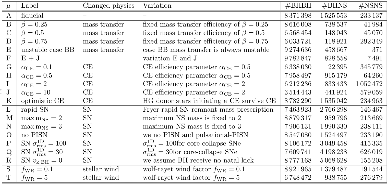
We use the simulations and methodology presented in 32. Here we add new models F, G, J, S and T, which leads to a minor shift in the model labels. Our models explore the key assumptions in both massive (binary) star evolution and , leading to ( binary stellar evolution ) model realizations. We particularly choose our model variations to explore a broad span of uncertainty in the modelling. For that reason some of the variations are somewhat extreme (e.g., models S and T), but are chosen to explore their possible impact on the rate and distribution shapes of DCO mergers. We summarize our most important model assumptions below and summarize the model variations in Table 1 (massive binary star evolution) and Table 2 (). More details can be found in the Appendix and in 32.
2.1 Massive binary-star population models
We simulate populations of GW sources with the rapid binary population synthesis code from the COMPAS11 1 Compact Object Mergers: Population Astrophysics and Statistics, https://compas.science suite (Stevenson et al. 2017; Barrett et al. 2018; Vigna-Gómez et al. 2018; Broekgaarden et al. 2019; Neijssel et al. 2019; Team COMPAS: J. Riley et al. 2021). We model the formation of BH and NS mergers from the isolated binary evolution channel where the merging DCO form from massive stars born in a binary system (Smarr & Blandford 1976; Srinivasan 1989). We explore uncertainties in our massive (binary) star evolution assumptions by studying binary population synthesis model variations. We further use the efficient sampling algorithm STROOPWAFEL (Broekgaarden et al. 2019) to simulate binary systems for 53 different values, resulting in typically DCO mergers in each simulation, making it one of the best-sampled population synthesis studies of its kind.
For our default model (A) settings we use the fiducial model summarized in 32. For the remaining models we change one population parameter at a time (relative to the fiducial model) to explore the impact of the uncertain model assumptions. The only exception is model F (E+K), which combines the model changes from both models E and K. Our models are summarized in Table 1 and we refer to them throughout the rest of the paper by the letters A to T and the abbreviated label names given in the second column of Table 1. We focus on (and decide to use) the stellar evolution and the variations mentioned below as these are commonly used in population synthesis settings, see Broekgaarden et al. 2021 for more details.
| Label | Variation | |
| A | fiducial | – |
| B | fixed mass transfer efficiency of | |
| C | fixed mass transfer efficiency of | |
| D | fixed mass transfer efficiency of | |
| E | unstable/no case BB | case BB mass transfer is always unstable |
| F | E + K | case BB mass transfer is always unstable |
| HG donor stars initiating a CE may survive | ||
| G | CE efficiency parameter | |
| H | CE efficiency parameter | |
| I | CE efficiency parameter | |
| J | CE efficiency parameter | |
| K | optimistic CE | HG donor stars initiating a CE may survive |
| L | rapid SN | Fryer rapid SN remnant mass model |
| M | maximum NS mass is fixed to | |
| N | maximum NS mass is fixed to | |
| O | no PISN | no PISN and pulsational-PISN |
| P | for core-collapse SNe | |
| Q | for core-collapse SNe | |
| R | we assume BH receive no natal kick | |
| S | Wolf-Rayet wind factor | |
| T | Wolf-Rayet wind factor |
.
In models B, C, D, E and F we explore uncertainties in binary mass transfer prescriptions. Of these, models B, C and D vary the mass transfer efficiency. This is defined in COMPAS by the parameter , which determines for a given donated mass rate the fraction that is accreted by the companion star: , with and being the mass of the accretor and donor stars, respectively, and the time (where is the simulation time step). The excess mass is assumed to leave the binary from the vicinity of the accreting star through ‘isotropic re-emission’ (Massevitch & Yungelson 1975; Bhattacharya & van den Heuvel 1991; Soberman et al. 1997, e.g.,) and the angular momentum loss is calculated accordingly (cf., Equations 32 and 33 in Belczynski et al. 2008). Our fiducial model (A) assumes the accretion rate is limited by the star’s thermal timescale: , where is the Kelvin-Helmholtz (thermal) timescale22 2 Given in Equation 61 of Hurley et al. 2002, where we use a pre-factor of 30 Myr from Equation 2 in Kalogera & Webbink 1996., and the factor of 10 is added to take into account the expansion of the accretor due to mass transfer (cf., Paczyński & Sienkiewicz 1972, Hurley et al. 2002 and Schneider et al. 2015). Models B, C and D assume a different accretion rate limit for stars by fixing to , , and , respectively. All of our models assume an Eddington-limited accretion rate for compact objects. In our fiducial model we assume that case BB mass transfer, which is mass transfer from a stripped post-helium-burning star onto the accretor (Delgado & Thomas 1981), is always stable. Model E explores a variation where case BB (and case BC, but these are more rare) mass transfer is assumed to always be unstable, leading to a CE phase. This assumption causes case BB mass transferring systems to merge as stars in model E as our fiducial model assumes the now unstable CE phase initiated by a (helium) Hertzsprung Gap star is unsuccessful and leads to a merger (as described further in the ‘pessimistic CE assumption’ in the next paragraph). We therefore also add model F, which explores the effect of assuming unstable case BB mass transfer, but allowing Hertzsprung Gap donor stars to survive a CE phase (the ‘optimistic CE assumption’).
In models G, H, I, J and K we explore the effect of changing the CE prescription assumptions, which in COMPAS are parameterized using the ‘–’ formalism from Webbink 1984 and de Kool 1990. Our fiducial model assumes a CE efficiency of and uses for the “Nanjing lambda” prescription (Dominik et al. 2012, cf.,), which is based on models from Xu & Li 2010a; Xu & Li 2010b. In models G, H, I and J we change the CE efficiency to fixed values of , , and , respectively. Compared to the fiducial model, lower and higher values of reduce and increase the efficiency with which the CE is ejected, respectively. In model K (and model F) we allow Hertzsprung gap stars that initiate a CE to possibly survive the CE (also known as the ‘optimistic’ CE assumption), whereas in our fiducial model these are assumed to always lead to an unsuccessful CE ejection (and merger), the ‘pessimistic’ CE scenario (Dominik et al. 2012, cf.,).
In models L, M, N, O, P, Q and R we vary the SN prescription assumptions. In model L we use the ‘rapid’ SN remnant mass model of Fryer et al. 2012 instead of their ‘delayed’ model, which is implemented in our fiducial model. The rapid model creates a mass gap between , where no BH form, whereas in the delayed model such BH can form. Models M and N change our assumption for the maximum NS mass, by default 2.5 , to and , respectively and we adapt the remnant mass prescription from Fryer et al. 2012 accordingly. In model O we do not use the prescription for pair-instability SN and pulsational pair-instability SN, therefore allowing the formation of BH in the mass range of . In models P and Q we change the root mean square velocity dispersion () for the Maxwellian SN natal kick distribution for both BH and NS, to 100 and 30, respectively (the fiducial model uses ). For all our models we assume that a fraction of the ejected material () falls back onto the compact object and we adjust the remnant mass and re-scale the SN kick magnitude accordingly (cf., Fryer et al. 2012). For ultra-stripped SN and electron-capture SN we always draw the SN kick using a one-dimensional root-mean-square velocity dispersion of following Pfahl et al. 2002 and Podsiadlowski et al. 2004. In model R we assume instead that only all BH receive zero natal kicks, .
Finally, models S and T explore the assumptions for the mass loss rate in Wolf-Rayet winds. Our Wolf-Rayet wind prescription follows Belczynski et al. 2010, which is based on Hamann & Koesterke 1998 and Vink & de Koter 2005, by parameterizing the wind strength with a multiplicative parameter (cf., Barrett et al. 2018). By default we use and in models S and T we vary this to and , respectively, which largely spans the possible range for Wolf-Rayet winds inferred from observations (e.g., Vink 2017; Hamann et al. 2019; Shenar et al. 2019; Sander & Vink 2020).
2.2 Metallicity-dependent star formation rate density models
The time between formation and merger of a DCO can range up to many Gyr (Neijssel et al. 2019, e.g.,). As a result, the DCO that are detected by current ground-based GW observatories can originate from stars that formed throughout a wide range of redshifts with a large variety of birth metallicities (Chruślińska & Nelemans 2019, e.g.,). Similar to 32, we follow the method of Neijssel et al. 2019 to create a metallicity-dependent star formation rate density , which describes the star formation history as a function of birth (initial) metallicity33 3 Where Z is the fractional metallicity, such that with X and Y the mass fractions of hydrogen and helium, respectively. and redshift . To explore uncertainties in , we use a total of models. Each model convolves a SFRD (SFRD)44 4 We use for the metallicity-dependent star formation rate density as a function of metallicity and redshift and SFRD for the total star formation rate density across all metallicities, which we model as only a function of redshift. with a metallicity probability distribution function, . Our first model (see Table 2 for the labeling) is the so-called ‘preferred’ phenomenological model from Neijssel et al. 2019, which they fit to match the BHBH observations from the first two observing runs by LIGO and Virgo. The other 27 () models are constructed by combining a SFRD with a GSMF (GSMF), and a MZR (MZR). The three variations for each SFRD, GSMF and MZR that we consider are given in Table 2. Although many of the prescriptions in these models oversimplify the complex that is evident from observations, these prescriptions provide a convenient parametrization for binary population synthesis studies. For more details about caveats and uncertainties in the modelling of within binary population synthesis we refer the reader to Chruślińska & Nelemans 2019, Neijssel et al. 2019, Boco et al. 2021 and references therein.
3 Results
3.1 Metallicity specific merger yields

In Figure 1 we show the calculated formation yields () for BHBH, BHNS and NSNS mergers per unit solar mass of stars formed () as a function of for our binary population synthesis models. This formation yield only includes DCO systems that have a GW driven inspiral time () that is smaller than the Hubble time () and is given by
| (1) |
where we convert the number of mergers in our COMPAS realizations to formation yields by integrating our simulation range over the full initial parameter space of binary systems (e.g., the full initial mass range of stars) and assuming a corrected55 5 Corrected to take into account the differences in parameter range between population synthesis and observations, see de Mink & Belczynski 2015. binary fraction of (Sana 2017, consistent with e.g.,). Details are given in 32.
3.1.1 Impact from the binary massive star evolution assumptions and metallicity
Figure 1 demonstrates that the variation in the BHBH merger formation yield is typically dominated by , causing variations on the order of between and . Variations in our massive binary population synthesis assumptions impact the BHBH merger yield only with factors of up to at and on the order of for most stellar evolution models at higher . The exceptions to this include model T (), which has a much lower BHBH yield (by ) compared to other stellar evolution models for where BH formation is drastically reduced due to the strong stellar wind mass loss. Other examples include the optimistic CE models (F and K) that have higher BHBH yields compared to other stellar evolution models for .
The scatter in the BHNS and NSNS formation yields, on the other hand, are typically dominated by variations in the stellar and binary evolution models over most of the range, leading to variations of in the rates, compared to typical ranges of from variations in for most models.
3.1.2 Trends in the metallicity-dependent formation yields
As can be seen in Figure 1, the formation yield of BHBH mergers is constant at low metallicities and then steeply declines at for all model variations. This steep decline of merging BHBHs at higher metallicities has been pointed out previously (Belczynski et al. 2010; Dominik et al. 2012, e.g.,), and is consistent with various recent works including Giacobbo et al. 2018, Giacobbo & Mapelli 2018, Klencki et al. 2018, Chruślińska & Nelemans 2019, Neijssel et al. 2019 and Santoliquido et al. 2021, demonstrating that this trend is present among many different population synthesis studies and simulation settings. This decline is due to several metallicity dependent effects. First, stronger stellar winds at higher metallicities lead to increased mass loss and hence wider binaries with less massive DCO, reducing the fraction of BHBH that will merge in a Hubble time. In addition, the less massive BH are assumed to have smaller amounts of fallback and hence receive larger natal kicks in our simulations, increasing the fraction that is disrupted during the SN (Fryer et al. 2012; Klencki et al. 2018; Renzo et al. 2019, cf.,). Indeed, in the model variations where BH receive lower or no SN kick (Q and R) or the Wolf-Rayet winds are weaker (model S) the decline in BHBH yield is less severe in Figure 1. Second, there is a metallicity dependence of the radius expansion of stars in our single star evolution tracks (Hurley et al. 2000), leading more stars to enter the CE phase during the Hertzsprung Gap instead of during the giant phase at higher () metallicities (cf., Figure 2 in Belczynski et al. 2010, Figure 7 in Linden et al. 2010 and Section 3.1.1 in Bavera et al. 2021). In our fiducial simulation such Hertzsprung Gap donor stars do not survive the CE phase. In models F (E+K) and K (optimistic CE) we instead assume these systems do survive, leading to a visible boost in BBH yields at higher , as seen in Figure 1.
The behavior of the BHNS yield in most models, on the other hand, first modestly increases as a function of and then declines around (Figure 1; cf., Klencki et al. 2018; Chruślińska & Nelemans 2019; Román-Garza et al. 2021). This causes the yield to broadly peak in the range , where the location of the peak varies between models as shown in Figure 1. The same metallicity dependent effects as described for BHBH mergers above are at play for BHNS mergers. However, since BHNS systems typically already form DCO with lower mass BH and form from lower mass stars compared to BHBH mergers, these BHNS systems do not experience the same boost in formation yields at low metallicities compared to the BHBH mergers, leading to lower yields at lower . In addition, the peak in BHNS yield is caused by the maximum radial extent of stars in the Hertzsprung Gap, which generally increases with but decreases between in our simulations for the zero-age main sequence mass range of BHNS progenitors (initial primary masses of ). This is based on the single star evolution prescriptions from Hurley et al. 2000 implemented in COMPAS. As a result of the smaller radii there are typically fewer stellar mergers in our simulations as fewer stars completely engulf their companion during mass transfer (Giacobbo & Mapelli 2018, as discussed by) and the average initial separations of binaries that form merging BHNS shifts to smaller values, which are more commonly formed. See also the discussion in §4.1.2 in Klencki et al. 2018 for additional details.
We find that the NSNS merger yield remains roughly constant as a function of (Chruślińska et al. 2018; Klencki et al. 2018; Giacobbo & Mapelli 2018; Neijssel et al. 2019, cf.,) as the metallicity-dependent effects described above are less significant for lower-mass stars that form NSNS binaries. The strong increase in formation yield around in Figure 1 that is particularly noticeable for NSNS binaries is due to a bifurcation in our prescription for the envelope binding energy (relevant for the CE phase) and is an artifact in our modelling. More orbital energy is needed to successfully unbind the envelope for in our models. This means that the binary engulfed in the CE will need to move to tighter orbits in order to successfully eject the envelope. This results in tighter post-CE binaries that survive the second SN and can merge in a Hubble time, thereby increasing the rate. Finally, we note that the scatter in model E (unstable case BB) is caused by sampling noise as a consequence of the very small number of NSNS mergers (only 371) in this simulation66 6 See our online table .. In the next Section we discuss this model and show that it under-predicts the inferred NSNS rate from GW observations by two orders of magnitude.
Comparing the panels in Figure 1 we find that at low the formation yield of merging BHBH in a Hubble time exceeds that of merging BHNS and NSNS. The merging BHNS formation yield starts dominating over the BHBH yield at , whereas for merging NSNS this occurs at for most models. We show these merging DCO ratios in Figure 11. Using our models we can translate these transition metallicities into approximate typical redshifts. For example, Figure 12 shows that the average metallicity of star formation is at and for the and models, respectively. These two models correspond to the highest and lowest average metallicity of star formation within our simulated models and, as we will show in the next section, to one of the lowest and highest DCO merger rate density predictions, respectively.
3.2 Intrinsic merger rates
In Figure 2 we show the population synthesis calculated local (intrinsic) merger rate densities for BHBH, BHNS and NSNS binaries. There are three main findings that we describe in more detail below. First, we find that the combined variations in our massive binary star and assumptions impact the intrinsic DCO rates with resulting ranges of . Second, only a subset of the models matches the ranges for the inferred BHBH, BHNS and NSNS merger rate density from GW observations (The LIGO Scientific Collaboration et al. 2021c). Third, we find that the calculated merger rates for different types of DCO are sensitive to different uncertainties in the modelling. Most strikingly, we find that the BHBH merger rates are primarily sensitive to variations in models, whereas the NSNS merger rates are predominantly impacted by binary stellar evolution model variations. This means that the observed BHBH and NSNS rates can provide a test-bed for and stellar evolution uncertainties, respectively.
The intrinsic rates are calculated using the formation yields from Equation 1 and by taking into account the weighting discussed in §2.2. The local merger rate is then obtained using in the equation (i.e. evaluating the equation at the center of our lowest redshift bin for )
| (2) |
where again is time in the source frame measured from the Big Bang77 7 Where we use the WMAP9–cosmology from Astropy (Hinshaw et al. 2013). This assumption does not drastically impact our results., is the time of the DCO merger, is the delay time between the formation of the DCO and its merger, and is the co-moving volume. The delay time is , the total time from the onset of hydrogen burning at ZAMS to forming a DCO, i.e., until the second SN (), and the time it takes the DCO to coalesce from the moment of the second SN (); see Figure 1 in 32 for more details. The binary initially forms at , which we set as in this equation. For the we use the models from Table 2. In practice we estimate Equation 2 with a Riemann sum where we sum over our metallicity grid and redshift (time) bins.
To quantify the scatter in the predicted intrinsic rates we calculate the mean of the ratios between the maximum and minimum predicted rates given by
| (3) |
and
| (4) |
where we used the short-hand notation and and are the stellar evolution and labels, respectively. Intuitively, Equation 3 represents the uncertainty range from stellar evolution as averaged over the models, whereas Equation 4 represents the uncertainty range from as averaged over the stellar evolution models. Large (small) values for and correspond to large (small) impacts by binary star evolution and variations, respectively.
3.2.1 BHBH merger rates
We find that the intrinsic merging BHBH rates are predicted to lie in the range as shown in the top panel in Figure 2. The combined uncertainty thus impacts the predicted rates with a factor of up to88 8 This is the ratio between the minimum and maximum predicted rates quoted with the error bar in the left of each panel in Figure 2. This is not the same as multiplying and , as the latter are averages calculated using Equations 3 and 4, and because the impacts from stellar evolution and variations are not (fully) independent. . We find that the variations in stellar and binary evolution impact the BHBH rate on average with , while variations in our models impact the predicted BHBH rate with uncertainties of .
We find that the majority of our stellar and binary evolution model variations do not impact the BHBH rate with more than a factor , as can be seen in the top panel of Figure 2 when comparing the predicted rates with our fiducial model. Model T () has the highest impact on the rates. The other largest BHBH rate changes are from stellar evolution models that change the CE assumptions (e.g., models F, G and K).
The credible intervals from the GW inferred rate of merging BHBH spans based on the GWTC-3 catalog from The LIGO Scientific Collaboration et al. 2021c99 9 From hereon we quote the rate range from the ‘merged’ row in Table II in The LIGO Scientific Collaboration et al. 2021c that represents the union of 90 credible intervals from their PDB, MS and BGP models.. Figure 2 shows that only a subset of our models (lower lines in the top panel) predict merging BHBH rates that are consistent with this range. The realizations that typically over-predict the observed BHBH rate for all stellar evolution models are the ones with an implementation of the Langer & Norman 2006 MZR . This MZR model corresponds to the lowest average among our MZR variations (right panel, Figure 12), which significantly increases the BHBH yield. The over-prediction is even more significant if other formation channels than the isolated binary evolution channel further contribute to the observed BHBH rate (Abbott et al. 2021b; Zevin et al. 2021, e.g.,).
3.2.2 BHNS merger rates
For the merging BHNS systems we find rates in the range as shown in the middle panel of Figure 2. Our combined model variations impact the predicted BHNS rates with an uncertainty factor of up to . We find that variations in the rate are typically for binary evolution variations, while the impact from variations typically leads to a range of .
Almost all predicted BHNS rates are consistent with the range spanned by the credible intervals from observations (The LIGO Scientific Collaboration et al. 2021c). The exceptions are a few of the models in combination with models D, E and G that under-predict the BHNS rate and a few of the models with in combination with stellar evolution model P, Q and R (lower SN kicks), which slightly over-predict the observed upper limit. The latter models have reduced SN kicks, which increases the fraction of systems that stay bound during the SN compared to our fiducial model (see 32 for a more detailed discussion). Future improved constraints might enable ruling out models.
3.2.3 NSNS merger rates
The bottom panel in Figure 2 shows our predicted merging NSNS rates. We find values in the range . Combined, our model realizations impact the estimated NSNS rates up to a factor of . The uncertainty from stellar and binary evolution dominates the scatter in the calculated NSNS rates (cf., Santoliquido et al. 2021), impacting the rate by compared to when varying the .
All of our calculated NSNS merger rates except those involving model E match the observed merger rate density range of (The LIGO Scientific Collaboration et al. 2021c), although the majority of rates fall in the lower end of the observed NSNS merger rate range. Models I, J, P and Q have the highest predicted NSNS merger rate densities as the NSNS rate is boosted in these models. For example, in models I and J fewer binaries merge during the CE phase compared to the fiducial model. In models P and Q the smaller value for the root-mean-square velocity dispersion reduces the kick velocities that decreases the number of binaries that disrupts during the SN. Only model E is in particular an outlier in the predicted NSNS merger rate. In this channel the formation yield of merging NSNS is extremely low (Figure 1). This is because the majority of systems leading to merging NSNS experience a case BB mass transfer phase that ultra-strips the NS progenitor (Dewi & Pols 2003; Tauris et al. 2017). In our model variation E we assume this phase of mass transfer to be unstable, leading to a stellar merger in combination with our pessimistic CE assumption. Indeed, in model F where we have the same settings as in model E but add the ‘optimistic’ CE assumptions, we obtain NSNS rates consistent with our fiducial model. If we exclude model E we find instead (while remains unchanged).
3.2.4 Trends with stellar evolution variations
There are a few trends visible in the rates in Figure 2. First, the predicted BHNS rate declines with increasing mass transfer efficiency, (models B, C and D). The increase in leads the secondary to accrete more mass during the first stable mass transfer phase, resulting in more massive secondaries and typically larger separations because the mass transfer is more conservative. The larger masses and/or larger separations at higher values results in more binaries eventually disrupting during a SN, merging during the CE phase, and/or forming a BHBH binary instead of a BHNS (cf., Kruckow et al. 2018). In addition, this also impacts in a complex way due to the interplay of the typically larger separation after the first stable mass transfer phase, as well as more orbital shrinking during the CE phase because the star has to eject a more massive envelope.
The BHBH and NSNS rates instead increase with increasing values for . This different behavior comes from a non-trivial combination of ways in which the formation pathways of binaries leading to merging BHNS are different from merging BHBH and NSNS and how changing impacts this. An example is that the impact from on the evolution of the binary is connected with the mass ratios of the binary (e.g. the mass ratio impacts the size of the Roche lobes, whether the mass transfer is stable or unstable and whether the mass transfer causes the binary orbit to widen or shrink). The merging BHBH and NSNS populations are DCO with more equal (i.e. ) mass ratio distributions compared to BHNS (see also §3.4). The binaries that form merging BHBH and NSNS originate thus from different mass ratio populations at the same evolutionary stages compared to merging BHNS. This results in the parameter impacting the populations differently. Another difference is that the merging BHNS typically form from different formation channels within isolated binary evolution compared to BHBH and NSNS. For example, in our fiducial model (A) a substantial fraction ( of all merging BHBH in our simulation) of the BHBH form through only stable mass transfer episodes, without engaging a CE, whereas for BHNS this is much smaller (). The parameter has a different impact on each of these formation channels.
Second, the BHNS rate increases with increasing values for (models G, H, I and J) as a result of more efficient ejection of the CE. This causes typically fewer systems to merge during the CE (cf., Kruckow et al. 2018, Figure 17). On the other hand, the rates slightly decline for the highest values as in this case binaries do not shrink enough to merge in a Hubble time (see also the discussion on in §3.1.1 from Bavera et al. 2021).
3.3 GW detectable merger rates
The top panel in Figure 3 shows the predicted detectable merger rates for our model variations. These are calculated by volume integrating Equation 2 and taking into account the sensitivity of a GW detector, quantified by the probability of observing a merging binary of specified masses at a given redshift and corresponding distance. Here we assume a detector sensitivity comparable to Advanced LIGO in its design configuration (hereafter, design sensitivity; LIGO Scientific Collaboration et al. 2015; Abbott et al. 2020a). We follow Barrett et al. 2018 and choose a detector signal-to-noise ratio threshold of 8 as a proxy for detectability by a GW detector network (e.g., LVK). The detectable merger rate is given by:
| (5) |
where is the time in the detector (i.e., the observer) frame, and and are the component masses of the DCO in the source frame (see 32 for further details).
Considering the model variations we find predicted detected rates for an LVK detector network at design sensitivity in the range , and , as shown in the top panel of Figure 3. We find that the stellar, binary, and cosmic evolution combined impact the predicted detectable merger rates by factors of up to . This is slightly higher compared to the intrinsic rates as the detectable population is biased to higher masses, where our simulations are relatively more sensitive to stellar evolution and assumptions.
3.3.1 Relative merger rates
The bottom panel of Figure 3 shows the relative merger rates between the different DCO channels for LVK at design sensitivity. We find that almost all of our models predict a higher BHNS detection rate compared to the NSNS detection rate, except for model D (which has a mass transfer efficiency of ) and model G (which assumes ) in which a subset of the models lead to higher NSNS detection rates. The higher BHNS rate is a result from both the high intrinsic yield of BHNS mergers compared to NSNS mergers (Figure 1) and the larger detection volume for BHNS compared to NSNS mergers as a result from their larger masses (§3.4).
3.4 GW detectable mass distribution functions
The uncertainties in stellar and binary evolution and also impact the shapes of the mass distributions of detectable DCO mergers, in addition to the overall merger rate densities. We show this in Figures 4 (BHBH), 5 (BHNS) and 6 (NSNS) for our model realizations. Each Figure shows the normalized distributions for the DCO component masses and , chirp mass , and mass ratio , where we use subscripts ‘1’ and ‘2’ to indicate the more massive and less massive component in the double compact object system, respectively. To compare the shapes we show kernel density distributions for the chirp mass and summary statistics (i.e., median, 50, and distribution percentiles) for the individual masses, chirp mass and mass ratio for the BHBH, BHNS and NSNS mergers. All distributions are weighted for the detection volume and sensitivity of LVK at design sensitivity using Equation 3.3 and given by the differential detectable merger rate , with being one of the mass parameters mentioned above.1010 10 From hereon we will use the short notation for this differential detection rate that describes the ‘shape’ of the distributions.


3.4.1 Impact from binary star and cosmic evolution on the distribution shapes
We qualitatively compare the impact on the shape of the detectable mass distributions from variations in stellar and binary evolution and variations in by analyzing how the distributions (and distribution statistics) vary; see Figures 4, 5 and 6. Distributions that are similar between vertical panels (different colors) indicate that changes in stellar and binary evolution assumptions do not significantly impact the distribution shape. On the other hand, distributions that are similar between variations plotted within one sub-panel indicate these realizations do not significantly impact the shape of the distributions. By comparing these two effects directly we can qualitatively analyze which of the two uncertainties dominates the shape of the detectable mass distributions.
For merging BHBH systems we find that the uncertainty in the shape of the mass distribution is significantly impacted by both variations in stellar evolution and the . The impact from the reflects the metallicity dependence of BHBH formation (§3.1), which also strongly impacts the resulting BH masses (Belczynski et al. 2010; Giacobbo & Mapelli 2018, cf.,). For example, the peak in the detectable BHBH chirp mass distribution around – that is visible in the majority of models in Figure 4 disappears in a small subset of the models. These are the models with the Panter et al. 2004 GSMF and Ma et al. 2016 MZR (113, 213 and 313), which correspond to realizations with high average metallicities compared to the other models (see Figure B1 in 32) and lead to fewer massive BHBH mergers. The stellar and binary evolution variation that impacts the mass distributions most drastically is the model in which we assume pair-instability SN do not occur (model O), leading to the formation of BH with masses . This model assumption may be unrealistic (Woosley 2017; Farmer et al. 2019, e.g.,). Other significant changes, best visible in the kernel density functions (left-most column in Figure 4), are present for models K (optimistic CE), L (rapid SN remnant model) and T (), where, for example, the chirp mass peaks shift, disappear or are created compared to the fiducial model A (e.g., in the ‘optimistic CE’ model due to the many additional BHBH systems added around lower chirp masses).
For merging BHNS systems, on the other hand, the distribution shapes are predominantly impacted by the stellar and binary evolution model variations compared to the variations (Figure 5). Primary effects include models E (unstable case BB), L (rapid SN), M (max ) and N (max ), where the median and distribution percentiles are visibly different compared to the fiducial model A. Our variations do not significantly impact the distribution shapes (i.e. changing more than a factor 2) for most of the models except model B, G and H.
For NSNS systems the shape of the normalized mass distributions are impacted by both sets of variations (Figure 6). Among the binary stellar evolution variations, the models that impact the shape of the distribution significantly are realizations that change the SN remnant mass or kick velocity, and/or the CE efficiency (models G, H, I, J, K, L, M, N, P and Q). The distributions from model E (unstable case BB mass transfer) are dominated by sampling noise as a result of the low NSNS yield in this model (§3.1). For the particularly all our models with the Langer & Norman 2006 MZR model () significantly impact the NSNS mass distributions, shifting the distributions to higher median masses in the panels of Figure 6.
In summary, we find that for BHNS, the variations in the distribution shapes are typically dominated by stellar and binary evolution assumptions, suggesting that observations of BHNS systems could aid in constraining stellar evolution models. For merging BHBH and NSNS the distribution shapes are impacted by both sets of variations (Figures 4 and 6). We therefore argue that constraining stellar evolution or models solely from the distribution shapes of merging BHBHs or NSNSs may be challenging. We discuss this further in §4.
3.4.2 Distribution properties considering all model realizations
In the previous section we showed that the model uncertainties in binary and stellar evolution, and can significantly impact the shapes of the DCO mass distributions. Here we instead discuss several specific examples of features in the mass distributions in Figures 4, 5 and 6 that are robust across all model variations explored in this work.
- •
First, in all model variations () of the detectable BHBH mergers have mass ratios () (right-most column in Figure 4). The BHBH distribution medians and percentiles furthermore indicate that in all model variations BHBH from isolated binary evolution prefer order unity mass ratios. Detecting a significant fraction () of BHBH mergers with large mass ratios () would point to other formation pathways or missing physics in our simulations. This is consistent with the 72 BHBH detections announced by LVK with a false alarm rate , which most of are inferred to have mass ratios consistent with unity (The LIGO Scientific Collaboration et al. 2021b). However, the BHBH merger GW190412 (; Abbott et al. 2020b) and the BHBH merger candidate GW190814 (; Abbott et al. 2020d), if common, could hint to the existence of a population with more extreme mass ratios (see also Arca Sedda 2021; Lu et al. 2021; Zevin et al. 2020a, and references therein).
- •
Second, of all BHBH mergers are expected to contain a BH with in all model variations (third column of Figure 4). This is not the case for BH in BHNS systems where typically of the detectable mergers are expected to contain a BH of (Figure 5). Our models predict the secondary BH in the population of detected BHBH mergers to also commonly be massive (), although many of our models do allow for at least of the BHBH mergers to contain a secondary BH with . For the currently reported BHBH detections by LVK with a false alarm rate (but even for those with a false alarm rate ) all of the inferred medians of the primary BH mass have BH masses (The LIGO Scientific Collaboration et al. 2021c, Table I), consistent with our models.
- •
Third, in all model variations of the detectable merging BHNS systems have BH masses (third column of Figure 5). As discussed in 32, this is due to the fact that more equal mass stars more readily survive important stellar evolution phases in the formation pathways to BHNS mergers; to form a BHNS one of the stars needs to be of sufficiently low mass to form a NS, leading to a preference for the other star to also be of lower mass than is typical in BHBH. Consequently, we find that in all our model realizations of BHNS mergers have chirp masses of . This suggests that detecting a BHNS merger with a BH mass could indicate that the system did not form from isolated binary evolution processes our models include, but instead from chemically homogeneous evolution and/or dynamical formation where such high BH masses are more commonly expected (Marchant et al. 2017; McKernan et al. 2020; Rastello et al. 2020, e.g.,). The two detected BHNS systems with a false alarm rate , GW200105 and GW200115, have (at the credible interval) (Abbott et al. 2021c) consistent with our models (Broekgaarden & Berger 2021; Broekgaarden et al. 2021, see also).
- •
Fourth, we find that in all model variations the NS in detectable NSNS mergers typically have lower NS masses compared to those in detectable BHNS mergers (Figures 5 and 6). We find this is true for both NS components in the NSNS mergers. This is again due to the preferrence for equal mass binaries to survive important evolutionary phases leading to BHNS formation, thereby favoring more massive pre-NS stars to form a BHNS system (see 32 for more details). To date two NSNS and BHNS detections have been announced by LVK with a false alarm rate (The LIGO Scientific Collaboration et al. 2021c). For the NSNS detections the NS masses are and (GW170817; Abbott et al. 2017) and and (GW190425; Abbott et al. 2020c), which may indicate a NSNS mass distribution that is not consistent with Galactic NSNS observations (Vigna-Gómez et al. 2018; The LIGO Scientific Collaboration et al. 2021c, e.g.). For the BHNS detections the NS masses were found to be (GW200105) and (GW200115) (Abbott et al. 2021c). More detections are needed to calculate robust median NS masses in NSNS and BHNS detections.
Besides the four specific points above, more common trends throughout our model variations are visible in Figures 4, 5 and 6, particularly in the lower and upper bounds for the BH and NS masses. Several of these trends, however, are direct results from the remnant mass prescriptions used in our models. For example, all models with the exception of model O (no PISN) predict that of the detected BHBH mergers have chirp masses in the range –. The upper limit is set by the maximum possible BH masses of allowed due to the implementation of pair-instability SN in our models (Marchant et al. 2019; Stevenson et al. 2019, e.g.,); in model O we do not implement pair-instability SN, and find BH masses up to about and BHBH chirp masses up to about . In addition, in most of our model realizations the majority of NS in NSNS mergers have masses of (consistent with e.g., Tauris et al. 2017; Vigna-Gómez et al. 2018). This is because many NSNS experience at least one ECSN (ECSN), which in COMPAS are mapped to a mass of (Timmes et al. 1996, Team COMPAS: J. Riley et al. 2021). In addition, many NSNS mergers in our models originate from relatively low mass stars with carbon-oxygen cores of at the time of the SN, which in the delayed SN remnant mass prescription are mapped to a fixed value of (Fryer et al. 2012). Combined, this results in a peak of NS masses at . Exceptions to this are the rapid SN remnant mass model (model I) where these low mass stars are instead mapped to NS masses of leading to a broader peak at . The lower and upper NS limits are also artificially set in our models to and , respectively (Fryer et al. 2012, cf.,), except in models M and N where we set the upper limit to 2 and 3, respectively.
3.5 Delay time and birth metallicity distributions


The uncertainties in the stellar evolution and prescriptions in population synthesis modelling can also impact the expected delay time () and birth metallicity () distributions of the detectable DCO mergers. We show the impact from the model realizations explored in this study in Figures 7, 8 and 9. We focus on the and distributions as these properties can be (indirectly) constrained from observations (Im et al. 2017; Safarzadeh et al. 2019; Fishbach & Kalogera 2021, e.g.,). In addition, these distributions provide insights into the range of birth metallicities and star formation redshifts that current GW observations probe, which can be informative for future modelling (e.g., help understand where to focus computational time and which to simulate). We note that impacts on the distribution also impact (indirectly) the distribution of , because the birth metallicity distribution (; §2.2) evolves as a function of redshift.
The most striking feature of the and distributions is that both are significantly impacted by the variations for all three DCO merger types. This is particularly discernible in the large scatter of the distribution percentiles (see each sub-panel). We find that the impact from models is particularly significant for our variations in the choice of the metallicity probability function (), which describes the distribution of birth metallicities of stars at a given redshift. This is because the birth metallicity strongly impacts the properties and rate of the DCO mergers, including through the metallicity-dependent formation yields, through mass loss that impact the DCO masses and can widen the orbit of the binary, and through the metallicity-dependent radial expansion of stars, which impacts mass transfer phases in our models (§3.1). In the convolution to obtain the detectable DCO mergers in Equation 3.3 all of these properties impact the resulting population. Thus, the and distributions of the detectable DCO mergers are significantly impacted by the choice of () and .
Variations in the stellar and binary evolution assumptions can also significantly impact the and distributions. For example, model T (), which increases the mass loss through stellar winds, drastically suppresses the number of BHBH and BHNS events that can form at higher metallicities (), thereby leading to fewer of the detectable BHBH and BHNS mergers forming from these metallicities (Figures 7 and 8). Another example is Model J (), which results in longer and lower compared to our fiducial model in Figures 8 and 9. In model J orbital angular momentum of the binary can much more efficiently be transformed into ejecting the CE. This leads to less orbital shrinking during the CE phase and longer inspiral times. As a result only BHNS and NSNS that formed early in the Universe with low have had long enough the time to inspiral and be detectable today. Model J does not impact the BHBH distributions as significantly because most detectable BHBH mergers in our simulations only go through stable mass transfer phases (as these produce more massive BHBH in our simulations that the detectable population is biased to, cf. van Son et al. 2021).
Overall, we find that the delay time distributions span a broad range between a few Myr and the Hubble time with possible peaks both at short () and long () delay times, reflecting contributions from binaries born at lower and higher redshifts, respectively. This is a result from the interplay between the being a function of redshift in combination with the DCO properties and formation efficiencies being dependent. We find that our model variations indicate that the detectable BHBH mergers (Figure 7) probe systems with the longest median delay times, compared to BHNS and NSNS mergers (Figures 8 and 9). However, exceptions exist, including model J () where the median delay times of detected BHNS and NSNS mergers are larger than those of BHBH mergers for the reasons discussed above.
For the birth metallicity distribution shapes the right panels of Figures 7, 8 and 9 show that the detectable DCO mergers arise from a broad range of birth metallicities. As expected from the formation yield efficiencies, BHBH mergers typically originate from the lowest birth metallicities, with most of our models having a median of , whereas the detectable BHNS and NSNS populations originate in our models from higher with most models having median of .
4 Discussion
4.1 A realistic view of population synthesis models
In this paper we demonstrate the importance of considering the uncertainties in both massive star and binary evolution, as well as the when aiming to learn about the formation, evolution, and mergers of binaries through a comparison of population synthesis models to GW observations. Here we discuss the implications of our results for interpreting population synthesis studies.
On the one hand, our findings provide a cautionary note for using GW observations to uncover stellar and binary evolution properties. Studies that draw conclusions by comparing population synthesis results with GW observations without considering the wide range of uncertainties in both stellar/binary evolution and assumptions could be drastically biased by the specific model realization that is chosen to derive the results (Belczynski et al. 2021; Bouffanais et al. 2021, cf.). For example, studies including Zevin et al. 2017, Bouffanais et al. 2019, Franciolini et al. 2021, Ng et al. 2021 and Zevin et al. 2021 aim to determine the contributions of different formation channels to the observed BHBH population. Further examples include Fragione 2021, which estimates the number of BHNS mergers with an electromagnetic counterpart. Our work shows that uncertainties in both stellar and binary evolution and modelling can drastically impact the rate and distribution shapes of the BHBH, BHNS and NSNS populations, challenging the ability to draw strong conclusions when only considering a few population synthesis models at this stage.
The situation is even more complex when considering that our larger suite of models ( realizations) still only represents a subset of the overall uncertainties in population synthesis studies. For example, even our broader set of models does not account for uncertainties in the stellar evolution tracks (Laplace et al. 2020; Agrawal et al. 2020, e.g.,), internal mixing (Schootemeijer et al. 2019, e.g.,), stellar rotation (de Mink & Mandel 2016; Mapelli et al. 2020, e.g.,), the more complex physics of the CE phase (Klencki et al. 2021; Ivanova et al. 2020; Marchant et al. 2021; Olejak et al. 2021, e.g.,), the additional possible remnant mass prescriptions (Dabrowny et al. 2021; Mandel et al. 2021, e.g.), the initial conditions of binary systems (de Mink & Belczynski 2015; Moe & Di Stefano 2017; Klencki et al. 2018, e.g.,), and the possible contributions from other formation channels (Zevin et al. 2021, e.g.,). In addition, there are model variations that we did not explore, including alternative analytical prescriptions (Chruślińska et al. 2019; Tang et al. 2020, e.g.,), prescriptions derived from cosmological (zoom-in) simulations (e.g., FIRE, Illustris, EAGLE, Millennium; Lamberts et al. 2016; Mapelli et al. 2017; du Buisson et al. 2020; Briel et al. 2021; Chu et al. 2021), and prescriptions inferred more directly from observations (Chruślińska & Nelemans 2019; Chruślińska et al. 2021, e.g., ).
On the other hand, the fact that model predictions are sensitive to the model assumptions also has positive consequences. As the true DCO merger rates and properties become more constrained by observations, then identifying which models are inconsistent with reality aids in excluding some combinations of model assumptions, and so helps to constrain stellar evolution and cosmic history. To do this we need to sufficiently understand how the uncertainties in our assumptions affect the model output. The results in this paper show that simultaneously modelling the impact of uncertainties from stellar evolution and on the rates and distribution shapes of all three DCO merger types can help. For example, in §3.2 we found that the BHBH merger rate densities predicted from binary population synthesis are relatively sensitive to uncertainties and might thereby present a good test bed to constrain prescriptions. Similarly, we found that the NSNS merger rate densities might be a good test bed to constrain stellar evolution models. These findings are in agreement with, and expand on, earlier work by Chruślińska et al. 2019; Neijssel et al. 2019; Tang et al. 2020; Santoliquido et al. 2021. Simultaneously comparing the predictions for all three DCO flavors can further aid in constraining models, as shown in Figure 2 for the merger rate densities. Another example is that we showed in §3.4 that the BHNS distribution shapes might particularly be a good test bed for stellar evolution models (Figure 5), whilst the shape of the mass distributions of BHBH and NSNS detections are impacted by both stellar evolution and our model assumptions (Figure 4). We emphasize that understanding to which uncertainty these different DCO observable properties are sensitive to also aids in understanding where to best spend computational time and work in the simulations. We showed in §3.4.2 that some population synthesis results are robust under our model variations. These features are important when identifying distinguishable characteristics of the isolated binary evolution channel compared to other formation channels. Constraining and learning from population synthesis models can be further aided in the future by additional constraints including those from redshift dependent rates and redshift dependent distribution shapes (Briel et al. 2021; Chu et al. 2021; Santoliquido et al. 2021, cf.) and additional observational constraints including those from electromagnetic observations of X-ray binaries (Belczynski et al. 2020; Vinciguerra et al. 2020, e.g.,), Galactic pulsar binaries (Kruckow et al. 2018; Vigna-Gómez et al. 2018; Chattopadhyay et al. 2020; Chattopadhyay et al. 2021, e.g.), short gamma-ray bursts (Mandhai et al. 2021; Zevin et al. 2020b, e.g.), or GW detections beyond LVK including Cosmic Explorer and LISA (Shao & Li 2018; Ng et al. 2021; Wagg et al. 2021, e.g.).
4.2 Comparison with GW mergers


At the time of writing the LVK collaboration published the latest GW catalog (GWTC-3; The LIGO Scientific Collaboration et al. 2021b) containing a total of 76 events with a false alarm rate of , consisting of 72 BHBH mergers, 2 NSNS mergers and 2 BHNS events The LIGO Scientific Collaboration et al. 2021c1111 11 We follow the most likely classification as reported in The LIGO Scientific Collaboration et al. 2021c. This includes classifying GW190814 as a BHBH event.. From these detections, the LVK inferred local merger rate densities1212 12 Assuming a merger rate constant in redshift. of , , and (The LIGO Scientific Collaboration et al. 2021c). We showed in Figure 2 that the majority of our model realizations match these inferred local merger rates. However, we also found that a subset of the models overestimate the BHBH merger rate, and that most of our models are at the lower end of the NSNS merger rate. If we scale our predicted merger ratios (Figure 3) to the 72 BHBH detections, we find a predicted range of BHNS and NSNS detections. Although these simulation ranges encompass the DCO numbers found in the GWTC-3 catalog, the majority of models seem to particularly underestimate the number of NSNS mergers. This is consistent with findings by other studies on isolated binary evolution populations (e.g., Giacobbo & Mapelli 2018; Chruślińska et al. 2018; Santoliquido et al. 2021), which indicated that matching the observed NSNS rate might require higher values for and/or smaller SN natal kicks. The NSNS rates could also relatively increase by changes in the mass transfer stability prescriptions () and envelope binding energy models (), which are not explored in our study (see Han et al. 2020; Lau et al. 2021, and references therein). Future observations and simulations can further constrain this.
Beyond the merger rates, GWTC-3 also provides the inferred mass distributions of the detected BHBH mergers. In Figure 10 we provide a comparison between the inferred BHBH chirp mass distribution and our set of simulations. We find that the majority of our models predict chirp mass distributions that are largely consistent with the inferred chirp mass distribution (and individual posterior distributions) for . Figure 10 shows that particularly the SN remnant mass model variations (model L, M, N and O) significantly impact the lower and higher chirp mass end of the distributions in this comparison. On the other hand, we find that most of model realizations do not match the several detected BHBH mergers with chirp masses . Examples include GW190521 with , GW190602 with , GW190620 with , GW190701 with and GW190706 with , which all have at least one component with an inferred median BH mass of , which is our implemented (pulsational) pair-instability SN BH mass limit. Moreover, even in model O, the model in which we assume that pair-instability SN do not occur, we find that of the detectable BHBH chirp masses are expected to be below (Figure 4), making it challenging to explain the inferred BH mass in GW190521 and the higher mass range of the chirp mass distribution as shown in Figure 10. The origin of these massive BH systems is still under debate. One possibility is that the location of the pair-instability mass gap could be shifted to higher masses (Spera & Mapelli 2017; Farmer et al. 2019; Farmer et al. 2020; Costa et al. 2021; Mehta et al. 2021; Woosley & Heger 2021, e.g.). Another possibility is that BHBH mergers with massive BH formed through channels other than the isolated binary evolution channel. For example, Tanikawa et al. 2021 showed that formation from population III stars can account for the missing high mass BHBH mergers in isolated binary evolution studies like ours that only model population I and II stars. Other formation channels have also been suggested for these massive BHBH mergers including hierarchical dynamical mergers (Rodriguez et al. 2015; Rodriguez et al. 2016; Anagnostou et al. 2020, e.g.), stellar mergers (Spera et al. 2019; Di Carlo et al. 2020; Kremer et al. 2020, e.g.), triples (Vigna-Gómez et al. 2021, e.g.) or mergers in AGN disks (Secunda et al. 2020, e.g.). For a more detailed discussion see, for example, Abbott et al. 2020e and Kimball et al. 2021 and references therein. Future studies should explore a full comparison with LVK data to further constrain models.
5 Conclusions
In this study we simulated the rates and properties of BHBH, BHNS and NSNS mergers detectable with existing GW detectors. We simultaneously examined the impact of two key modelling uncertainties in population synthesis studies: uncertainties arising from massive binary star evolution, and from the metallicity-dependent star formation history, . We accomplish this by simulating populations of binaries over a grid of 53 birth metallicity values and taking into account the and GW detection probability. The resulting suite of model realizations ( binary stellar evolution variations variations) is the largest of its kind, and made publicly available. Our main findings within the context of the variations we considered are summarized below.
- •
Merging DCO formation yields: We find for all our stellar evolution variations that the merging BHBH (BHNS) formation yield is typically a rapidly decreasing function of metallicity at () as a result of line-driven Wolf-Rayet like winds. The NSNS yield, on the other hand, is relatively independent of metallicity. We find that the formation yield of BHBH mergers for is remarkably constant over massive binary-star models and . The formation yields of BHNS and NSNS mergers are impacted over the full metallicity range by our massive binary-star assumptions (see Figure 1).
- •
Merging DCO rates: We find that the calculated intrinsic and detectable merger rate densities ( and , respectively) can be impacted by factors – due to combined uncertainties in stellar evolution and . The model variations lead to estimated merger rate densities in the ranges – and – for BHBH, – and – for BHNS, and – and – for NSNS, for a ground-based GW detector consisting of LIGO-Virgo-KAGRA at design sensitivity. In particular, we found that the estimated BHBH merger rate densities are relatively sensitive to our explored uncertainties and might thereby present a good test bed to constrain prescriptions. On the other hand, we found that the NSNS merger rate densities are sensitive to stellar evolution models and therefore might be a good test bed to constrain stellar evolution models. For BHNS we find that the calculated rates are significantly impacted by both uncertainties (see Figures 2 and 3).
- •
Merging DCO mass distribution shapes: We show in Figures 4, 5 and 6 the impact from the massive binary-star and variations on the (normalized) shape of the detectable DCO mass distributions (chirp mass, individual component masses and mass ratios). We find that the shape of the BHNS mass distributions are dominated by variations in binary stellar evolution within our model explorations. For BHBH and NSNS mergers we find that the mass distribution shapes are impacted by both variations in stellar evolution and .
- •
Merging DCO and distribution shapes: We show in Figures 7, 8 and 9 the impact from binary stellar evolution and variations on the delay time and birth metallicity distributions calculated in our models. We find that the has a significant impact for BHBH, BHNS and NSNS on the shape of the delay time and metallicity distributions of detectable mergers. Several stellar evolution models, including those affecting stellar winds, can also significantly impact the delay time and distribution shapes.
- •
Consistent features among our model variations: We find several features in the DCO mass distributions that are consistent among all our model variations. First, we find that at least of the detectable BHBH mergers have mass ratios in all model variations (fifth column Figure 4). Second, we find that more than of BHBH mergers are always expected to contain a BH with a mass (third column Figure 4). Third, we find that less than of the detectable merging BHNS systems have BH masses (third column Figure 5). Fourth we find that NS in NSNS mergers are expected to have lower masses on average compared to NS in BHNS mergers (Figures 5 and 6). We discuss how these findings are marginally consistent with GW observations from GWTC-3 in §3.4.2 and §4.2.
Overall, our results highlight the importance of considering the uncertainty in both the stellar evolution and metallicity-dependent star formation history when exploring population synthesis simulations of BHNS, BHBH and NSNS mergers and when trying to infer model properties from GW data.
Acknowledgements
The authors thank everyone in the COMPAS collaboration and Berger Time-Domain Group for help. In addition, the authors thank the Harvard FAS research computing group for technical support on the simulations and high performance computing part of the research. The authors also thank Shanika Galaudage and Victoria DiTomasso for their help with this paper. FSB thanks Christopher Brown and Katie Callam for organizing the ‘writing oasis’. Lastly, FSB wants to acknowledge the amount of serendipity and privilege that was involved to end up pursuing this astronomy research. The Berger Time-Domain Group is supported in part by NSF and NASA grants. Some of the authors are supported by the Australian Research Council Centre of Excellence for Gravitational Wave Discovery (OzGrav), through project number CE170100004. FSB is supported in part by the Prins Bernard Cultuurfonds studiebeurs 2021. IM is a recipient of the Australian Research Council Future Fellowship FT190100574. A.V-G. acknowledges funding support by the Danish National Research Foundation (DNRF132). SJ, LvS and SdM acknowledge funding from the Netherlands Organisation for Scientific Research (NWO), as part of the Vidi research program BinWaves (project number 639.042.728) and the European Union’s Horizon 2020 research and innovation program from the European Research Council (ERC, Grant agreement No. 715063). LvS, TW and SdM acknowledge support by the National Science Foundation under Grant No. (NSF 2009131). This research has made use of NASA’s Astrophysics Data System Bibliographic Services. This research has made use of data, software and/or web tools obtained from the Gravitational Wave Open Science Center (https://www.gw-openscience.org/), a service of LIGO Laboratory, the LIGO Scientific Collaboration and the Virgo Collaboration. LIGO Laboratory and Advanced LIGO (LIGO Scientific Collaboration et al. 2015) are funded by the United States National Science Foundation (NSF) as well as the Science and Technology Facilities Council (STFC) of the United Kingdom, the Max-Planck-Society (MPS), and the State of Niedersachsen/Germany for support of the construction of Advanced LIGO and construction and operation of the GEO600 detector. Additional support for Advanced LIGO was provided by the Australian Research Council. Virgo (Acernese et al. 2015) is funded, through the European Gravitational Observatory (EGO), by the French Centre National de Recherche Scientifique (CNRS), the Italian Istituto Nazionale di Fisica Nucleare (INFN) and the Dutch Nikhef, with contributions by institutions from Belgium, Germany, Greece, Hungary, Ireland, Japan, Monaco, Poland, Portugal, Spain (The LIGO Scientific Collaboration et al. 2021a).
Data availability
All data used in this work is publicly available on Zenodo at Broekgaarden 2021a Broekgaarden 2021b and Broekgaarden 2021c. All code to reproduce the results and figures in this paper (and additional figures) are publicly available on Github at https://github.com/FloorBroekgaarden/Double-Compact-Object-Mergers .
Software
Simulations in this paper made use of the COMPAS rapid binary population synthesis code, which is freely available at http://github.com/TeamCOMPAS/COMPAS (Team COMPAS: J. Riley et al. 2021) including work based on (Stevenson et al. 2017; Barrett et al. 2018; Vigna-Gómez et al. 2018; Broekgaarden et al. 2019). The simulations performed in this work were simulated with a COMPAS version that predates the publicly available code. Our version of the code is most similar to version 02.13.01 of the publicly available COMPAS code. Requests for the original code can be made to the lead author. The authors used STROOPWAFEL from (Broekgaarden et al. 2019), publicly available at https://github.com/FloorBroekgaarden/STROOPWAFEL1313 13 For the latest pip installable version of STROOPWAFEL please contact the corresponding author..
The authors made use of Python from the Python Software Foundation. Python Language Reference, version 3.6. Available at http://www.python.org (van Rossum 1995). In addition the following Python packages were used: matplotlib (Hunter 2007), NumPy (Harris et al. 2020), SciPy (Virtanen et al. 2020), ipythonjupyter (Perez & Granger 2007; Kluyver et al. 2016), pandas (Wes McKinney 2010), Seaborn (Waskom & the seaborn development team 2020), Astropy (Astropy Collaboration et al. 2018) and hdf5 (Collette 2013).
Figure 10 makes use of the makeplotsVamana.py code by Vaibhav Tiwari on behalf of the LIGO Scientific Collaboration, Virgo Collaboration and KAGRA Collaboration provided under the Creative Commons Attribution 4.0 licence. We obtained their code from Zenodo doi:10.5281/zenodo.5655785, which makes use of the kernel density estimator as provided in https://dcc.ligo.org/LIGO-T2100447/public (Sadiq et al. 2021). The simulations were performed on the super computers from the Harvard FAS research computing group.
References
- Abbott et al. (2017) Abbott B. P., et al., 2017, Phys. Rev. Lett., 119, 161101
- Abbott et al. (2019) Abbott B. P., et al., 2019, Physical Review X, 9, 031040
- Abbott et al. (2020a) Abbott B. P., Abbott R., Abbott T. D., others Zweizig J., 2020a, Living Reviews in Relativity, 23, 3
- Abbott et al. (2020b) Abbott R., et al., 2020b, Phys. Rev. D, 102, 043015
- Abbott et al. (2020c) Abbott B. P., et al., 2020c, ApJ, 892, L3
- Abbott et al. (2020d) Abbott R., et al., 2020d, ApJ, 896, L44
- Abbott et al. (2020e) Abbott R., et al., 2020e, ApJ, 900, L13
- Abbott et al. (2021a) Abbott R., et al., 2021a, Physical Review X, 11, 021053
- Abbott et al. (2021b) Abbott R., et al., 2021b, ApJ, 913, L7
- Abbott et al. (2021c) Abbott R., et al., 2021c, ApJ, 915, L5
- Acernese et al. (2015) Acernese F., et al., 2015, Classical and Quantum Gravity, 32, 024001
- Agrawal et al. (2020) Agrawal P., Hurley J., Stevenson S., Szécsi D., Flynn C., 2020, MNRAS, 497, 4549
- Anagnostou et al. (2020) Anagnostou O., Trenti M., Melatos A., 2020, arXiv e-prints, p. arXiv:2010.06161
- Arca Sedda (2021) Arca Sedda M., 2021, ApJ, 908, L38
- Astropy Collaboration et al. (2018) Astropy Collaboration et al., 2018, AJ, 156, 123
- Barrett et al. (2018) Barrett J. W., Gaebel S. M., Neijssel C. J., Vigna-Gómez A., Stevenson S., Berry C. P. L., Farr W. M., Mandel I., 2018, MNRAS, 477, 4685
- Bavera et al. (2021) Bavera S. S., et al., 2021, A&A, 647, A153
- Belczynski et al. (2008) Belczynski K., Kalogera V., Rasio F. A., Taam R. E., Zezas A., Bulik T., Maccarone T. J., Ivanova N., 2008, ApJS, 174, 223
- Belczynski et al. (2010) Belczynski K., Dominik M., Bulik T., O’Shaughnessy R., Fryer C., Holz D. E., 2010, ApJ, 715, L138
- Belczynski et al. (2020) Belczynski K., et al., 2020, A&A, 636, A104
- Belczynski et al. (2021) Belczynski K., et al., 2021, arXiv e-prints, p. arXiv:2108.10885
- Bhattacharya & van den Heuvel (1991) Bhattacharya D., van den Heuvel E. P. J., 1991, Phys. Rep., 203, 1
- Boco et al. (2021) Boco L., Lapi A., Chruslinska M., Donevski D., Sicilia A., Danese L., 2021, ApJ, 907, 110
- Bouffanais et al. (2019) Bouffanais Y., Mapelli M., Gerosa D., Di Carlo U. N., Giacobbo N., Berti E., Baibhav V., 2019, ApJ, 886, 25
- Bouffanais et al. (2021) Bouffanais Y., Mapelli M., Santoliquido F., Giacobbo N., Di Carlo U. N., Rastello S., Artale M. C., Iorio G., 2021, MNRAS, 507, 5224
- Briel et al. (2021) Briel M. M., Eldridge J. J., Stanway E. R., Stevance H. F., Chrimes A. A., 2021, arXiv e-prints, p. arXiv:2111.08124
- Broekgaarden (2021a) Broekgaarden F. S., 2021a, BHBH simulations from: Impact of Massive Binary Star and Cosmic Evolution on Gravitational Wave Observations II: Double Compact Object Mergers, doi:10.5281/zenodo.5651073, https://doi.org/10.5281/zenodo.5651073
- Broekgaarden (2021b) Broekgaarden F. S., 2021b, BHNS simulations from: Impact of Massive Binary Star and Cosmic Evolution on Gravitational Wave Observations II: Double Compact Object Mergers, doi:10.5281/zenodo.5178777, https://doi.org/10.5281/zenodo.5178777
- Broekgaarden (2021c) Broekgaarden F. S., 2021c, NSNS simulations from: Impact of Massive Binary Star and Cosmic Evolution on Gravitational Wave Observations II: Double Compact Object Mergers, doi:10.5281/zenodo.5189849, https://doi.org/10.5281/zenodo.5189849
- Broekgaarden & Berger (2021) Broekgaarden F. S., Berger E., 2021, ApJ, 920, L13
- Broekgaarden et al. (2019) Broekgaarden F. S., et al., 2019, MNRAS, 490, 5228
- Broekgaarden et al. (2021) Broekgaarden F. S., et al., 2021, MNRAS,
- Chattopadhyay et al. (2020) Chattopadhyay D., Stevenson S., Hurley J. R., Rossi L. J., Flynn C., 2020, MNRAS, 494, 1587
- Chattopadhyay et al. (2021) Chattopadhyay D., Stevenson S., Hurley J. R., Bailes M., Broekgaarden F., 2021, MNRAS, 504, 3682
- Chruślińska & Nelemans (2019) Chruślińska M., Nelemans G., 2019, MNRAS, 488, 5300
- Chruślińska et al. (2018) Chruślińska M., Belczynski K., Klencki J., Benacquista M., 2018, MNRAS, 474, 2937
- Chruślińska et al. (2019) Chruślińska M., Nelemans G., Belczynski K., 2019, MNRAS, 482, 5012
- Chruślińska et al. (2021) Chruślińska M., Nelemans G., Boco L., Lapi A., 2021, MNRAS,
- Chu et al. (2021) Chu Q., Yu S., Lu Y., 2021, MNRAS,
- Collette (2013) Collette A., 2013, Python and HDF5. O’Reilly
- Costa et al. (2021) Costa G., Bressan A., Mapelli M., Marigo P., Iorio G., Spera M., 2021, MNRAS, 501, 4514
- Dabrowny et al. (2021) Dabrowny M., Giacobbo N., Gerosa D., 2021, Rendiconti Lincei. Scienze Fisiche e Naturali,
- de Kool (1990) de Kool M., 1990, ApJ, 358, 189
- de Mink & Belczynski (2015) de Mink S. E., Belczynski K., 2015, ApJ, 814, 58
- de Mink & Mandel (2016) de Mink S. E., Mandel I., 2016, MNRAS, 460, 3545
- Delgado & Thomas (1981) Delgado A. J., Thomas H. C., 1981, A&A, 96, 142
- Dewi & Pols (2003) Dewi J. D. M., Pols O. R., 2003, MNRAS, 344, 629
- Di Carlo et al. (2020) Di Carlo U. N., Mapelli M., Bouffanais Y., Giacobbo N., Santoliquido F., Bressan A., Spera M., Haardt F., 2020, MNRAS, 497, 1043
- Dominik et al. (2012) Dominik M., Belczynski K., Fryer C., Holz D. E., Berti E., Bulik T., Mand el I., O’Shaughnessy R., 2012, ApJ, 759, 52
- Dominik et al. (2015) Dominik M., et al., 2015, ApJ, 806, 263
- du Buisson et al. (2020) du Buisson L., et al., 2020, MNRAS, 499, 5941
- Farmer et al. (2019) Farmer R., Renzo M., de Mink S. E., Marchant P., Justham S., 2019, ApJ, 887, 53
- Farmer et al. (2020) Farmer R., Renzo M., de Mink S. E., Fishbach M., Justham S., 2020, ApJ, 902, L36
- Fishbach & Kalogera (2021) Fishbach M., Kalogera V., 2021, ApJ, 914, L30
- Fragione (2021) Fragione G., 2021, arXiv e-prints, p. arXiv:2110.09604
- Franciolini et al. (2021) Franciolini G., et al., 2021, arXiv e-prints, p. arXiv:2105.03349
- Fryer et al. (2012) Fryer C. L., Belczynski K., Wiktorowicz G., Dominik M., Kalogera V., Holz D. E., 2012, ApJ, 749, 91
- Furlong et al. (2015) Furlong M., et al., 2015, MNRAS, 450, 4486
- Giacobbo & Mapelli (2018) Giacobbo N., Mapelli M., 2018, MNRAS, 480, 2011
- Giacobbo et al. (2018) Giacobbo N., Mapelli M., Spera M., 2018, MNRAS, 474, 2959
- Hamann & Koesterke (1998) Hamann W. R., Koesterke L., 1998, A&A, 335, 1003
- Hamann et al. (2019) Hamann W. R., et al., 2019, A&A, 625, A57
- Han et al. (2020) Han Z.-W., Ge H.-W., Chen X.-F., Chen H.-L., 2020, Research in Astronomy and Astrophysics, 20, 161
- Harris et al. (2020) Harris C. R., et al., 2020, Nature, 585, 357–362
- Hinshaw et al. (2013) Hinshaw G., et al., 2013, ApJS, 208, 19
- Hunter (2007) Hunter J. D., 2007, Computing in Science and Engineering, 9, 90
- Hurley et al. (2000) Hurley J. R., Pols O. R., Tout C. A., 2000, MNRAS, 315, 543
- Hurley et al. (2002) Hurley J. R., Tout C. A., Pols O. R., 2002, MNRAS, 329, 897
- Im et al. (2017) Im M., et al., 2017, ApJ, 849, L16
- Ivanova et al. (2020) Ivanova N., Justham S., Ricker P., 2020, Common Envelope Evolution, doi:10.1088/2514-3433/abb6f0.
- Kalogera & Webbink (1996) Kalogera V., Webbink R. F., 1996, ApJ, 458, 301
- Kimball et al. (2021) Kimball C., et al., 2021, ApJ, 915, L35
- Klencki et al. (2018) Klencki J., Moe M., Gladysz W., Chruslinska M., Holz D. E., Belczynski K., 2018, A&A, 619, A77
- Klencki et al. (2021) Klencki J., Nelemans G., Istrate A. G., Chruslinska M., 2021, A&A, 645, A54
- Kluyver et al. (2016) Kluyver T., et al., 2016, in ELPUB. pp 87–90
- Kremer et al. (2020) Kremer K., et al., 2020, ApJ, 903, 45
- Kruckow et al. (2018) Kruckow M. U., Tauris T. M., Langer N., Kramer M., Izzard R. G., 2018, MNRAS, 481, 1908
- LIGO Scientific Collaboration et al. (2015) LIGO Scientific Collaboration et al., 2015, Classical and Quantum Gravity, 32, 074001
- Lamberts et al. (2016) Lamberts A., Garrison-Kimmel S., Clausen D. R., Hopkins P. F., 2016, MNRAS, 463, L31
- Langer & Norman (2006) Langer N., Norman C. A., 2006, ApJ, 638, L63
- Laplace et al. (2020) Laplace E., Götberg Y., de Mink S. E., Justham S., Farmer R., 2020, A&A, 637, A6
- Lau et al. (2021) Lau M. Y. M., Hirai R., González-Bolívar M., Price D. J., De Marco O., Mandel I., 2021, arXiv e-prints, p. arXiv:2111.00923
- Linden et al. (2010) Linden T., Kalogera V., Sepinsky J. F., Prestwich A., Zezas A., Gallagher J. S., 2010, ApJ, 725, 1984
- Lu et al. (2021) Lu W., Beniamini P., Bonnerot C., 2021, MNRAS, 500, 1817
- Ma et al. (2016) Ma X., Hopkins P. F., Faucher-Giguère C.-A., Zolman N., Muratov A. L., Kereš D., Quataert E., 2016, MNRAS, 456, 2140
- Madau & Dickinson (2014) Madau P., Dickinson M., 2014, ARA&A, 52, 415
- Madau & Fragos (2017) Madau P., Fragos T., 2017, ApJ, 840, 39
- Mandel & Broekgaarden (2021) Mandel I., Broekgaarden F. S., 2021, arXiv e-prints, p. arXiv:2107.14239
- Mandel & Farmer (2018) Mandel I., Farmer A., 2018, arXiv e-prints, p. arXiv:1806.05820
- Mandel et al. (2021) Mandel I., Müller B., Riley J., de Mink S. E., Vigna-Gómez A., Chattopadhyay D., 2021, MNRAS, 500, 1380
- Mandhai et al. (2021) Mandhai S., Lamb G. P., Tanvir N. R., Bray J., Nixon C. J., Eyles-Ferris R. A. J., Levan A. J., Gompertz B. P., 2021, arXiv e-prints, p. arXiv:2109.09714
- Mapelli (2021) Mapelli M., 2021, Formation Channels of Single and Binary Stellar-Mass Black Holes. p. 4, doi:10.1007/978-981-15-4702-7_16-1
- Mapelli et al. (2017) Mapelli M., Giacobbo N., Ripamonti E., Spera M., 2017, MNRAS, 472, 2422
- Mapelli et al. (2020) Mapelli M., Spera M., Montanari E., Limongi M., Chieffi A., Giacobbo N., Bressan A., Bouffanais Y., 2020, ApJ, 888, 76
- Marchant et al. (2017) Marchant P., Langer N., Podsiadlowski P., Tauris T. M., de Mink S., Mandel I., Moriya T. J., 2017, A&A, 604, A55
- Marchant et al. (2019) Marchant P., Renzo M., Farmer R., Pappas K. M. W., Taam R. E., de Mink S. E., Kalogera V., 2019, ApJ, 882, 36
- Marchant et al. (2021) Marchant P., Pappas K. M. W., Gallegos-Garcia M., Berry C. P. L., Taam R. E., Kalogera V., Podsiadlowski P., 2021, A&A, 650, A107
- Massevitch & Yungelson (1975) Massevitch A., Yungelson L., 1975, Mem. Soc. Astron. Italiana, 46, 217
- McKernan et al. (2020) McKernan B., Ford K. E. S., O’Shaughnessy R., 2020, MNRAS, 498, 4088
- Mehta et al. (2021) Mehta A. K., Buonanno A., Gair J., Miller M. C., Farag E., deBoer R. J., Wiescher M., Timmes F. X., 2021, arXiv e-prints, p. arXiv:2105.06366
- Moe & Di Stefano (2017) Moe M., Di Stefano R., 2017, The Astrophysical Journal Supplement Series, 230, 15
- Neijssel et al. (2019) Neijssel C. J., et al., 2019, MNRAS, 490, 3740
- Ng et al. (2021) Ng K. K. Y., Vitale S., Farr W. M., Rodriguez C. L., 2021, ApJ, 913, L5
- Olejak et al. (2021) Olejak A., Belczynski K., Ivanova N., 2021, A&A, 651, A100
- Paczyński & Sienkiewicz (1972) Paczyński B., Sienkiewicz R., 1972, Acta Astron., 22, 73
- Panter et al. (2004) Panter B., Heavens A. F., Jimenez R., 2004, MNRAS, 355, 764
- Perez & Granger (2007) Perez F., Granger B. E., 2007, Computing in Science and Engineering, 9, 21
- Pfahl et al. (2002) Pfahl E., Rappaport S., Podsiadlowski P., 2002, ApJ, 571, L37
- Podsiadlowski et al. (2004) Podsiadlowski P., Langer N., Poelarends A. J. T., Rappaport S., Heger A., Pfahl E., 2004, ApJ, 612, 1044
- Rastello et al. (2020) Rastello S., Mapelli M., Di Carlo U. N., Giacobbo N., Santoliquido F., Spera M., Ballone A., Iorio G., 2020, MNRAS, 497, 1563
- Renzo et al. (2019) Renzo M., et al., 2019, A&A, 624, A66
- Rodriguez et al. (2015) Rodriguez C. L., Morscher M., Pattabiraman B., Chatterjee S., Haster C.-J., Rasio F. A., 2015, Phys. Rev. Lett., 115, 051101
- Rodriguez et al. (2016) Rodriguez C. L., Chatterjee S., Rasio F. A., 2016, Phys. Rev. D, 93, 084029
- Román-Garza et al. (2021) Román-Garza J., et al., 2021, ApJ, 912, L23
- Sadiq et al. (2021) Sadiq J., Dent T., Wysocki D., 2021, Available as LIGO-T2100447
- Safarzadeh et al. (2019) Safarzadeh M., Berger E., Ng K. K. Y., Chen H.-Y., Vitale S., Whittle C., Scannapieco E., 2019, ApJ, 878, L13
- Sana (2017) Sana H., 2017, in Eldridge J. J., Bray J. C., McClelland L. A. S., Xiao L., eds, IAU Symposium Vol. 329, The Lives and Death-Throes of Massive Stars. pp 110–117 (arXiv:1703.01608), doi:10.1017/S1743921317003209
- Sander & Vink (2020) Sander A. A. C., Vink J. S., 2020, MNRAS, 499, 873
- Santoliquido et al. (2021) Santoliquido F., Mapelli M., Giacobbo N., Bouffanais Y., Artale M. C., 2021, MNRAS, 502, 4877
- Schneider et al. (2015) Schneider F. R. N., Izzard R. G., Langer N., de Mink S. E., 2015, ApJ, 805, 20
- Schootemeijer et al. (2019) Schootemeijer A., Langer N., Grin N. J., Wang C., 2019, A&A, 625, A132
- Secunda et al. (2020) Secunda A., et al., 2020, ApJ, 903, 133
- Shao & Li (2018) Shao Y., Li X.-D., 2018, ApJ, 867, 124
- Shenar et al. (2019) Shenar T., et al., 2019, A&A, 627, A151
- Smarr & Blandford (1976) Smarr L. L., Blandford R., 1976, ApJ, 207, 574
- Soberman et al. (1997) Soberman G. E., Phinney E. S., van den Heuvel E. P. J., 1997, A&A, 327, 620
- Spera & Mapelli (2017) Spera M., Mapelli M., 2017, MNRAS, 470, 4739
- Spera et al. (2019) Spera M., Mapelli M., Giacobbo N., Trani A. A., Bressan A., Costa G., 2019, MNRAS, 485, 889
- Srinivasan (1989) Srinivasan G., 1989, A&ARv, 1, 209
- Stevenson et al. (2017) Stevenson S., Vigna-Gómez A., Mandel I., Barrett J. W., Neijssel C. J., Perkins D., de Mink S. E., 2017, Nature Communications, 8, 14906
- Stevenson et al. (2019) Stevenson S., Sampson M., Powell J., Vigna-Gómez A., Neijssel C. J., Szécsi D., Mandel I., 2019, ApJ, 882, 121
- Strolger et al. (2004) Strolger L.-G., et al., 2004, ApJ, 613, 200
- Tang et al. (2020) Tang P. N., Eldridge J. J., Stanway E. R., Bray J. C., 2020, MNRAS, 493, L6
- Tanikawa et al. (2021) Tanikawa A., Yoshida T., Kinugawa T., Trani A. A., Hosokawa T., Susa H., Omukai K., 2021, arXiv e-prints, p. arXiv:2110.10846
- Tauris et al. (2017) Tauris T. M., et al., 2017, ApJ, 846, 170
- Team COMPAS: J. Riley et al. (2021) Team COMPAS: J. Riley et al., 2021, arXiv e-prints, p. arXiv:2109.10352
- The LIGO Scientific Collaboration et al. (2021a) The LIGO Scientific Collaboration the Virgo Collaboration the KAGRA Collaboration 2021a, The population of merging compact binaries inferred using gravitational waves through GWTC-3 - Data release, doi:10.5281/zenodo.5655785, https://doi.org/10.5281/zenodo.5655785
- The LIGO Scientific Collaboration et al. (2021b) The LIGO Scientific Collaboration et al., 2021b, arXiv e-prints, p. arXiv:2111.03606
- The LIGO Scientific Collaboration et al. (2021c) The LIGO Scientific Collaboration et al., 2021c, arXiv e-prints, p. arXiv:2111.03634
- Timmes et al. (1996) Timmes F. X., Woosley S. E., Weaver T. A., 1996, ApJ, 457, 834
- van Rossum (1995) van Rossum G., 1995, Technical Report CS-R9526, Python tutorial. Centrum voor Wiskunde en Informatica (CWI), Amsterdam
- van Son et al. (2021) van Son L. A. C., et al., 2021, arXiv e-prints, p. arXiv:2110.01634
- Vigna-Gómez et al. (2018) Vigna-Gómez A., et al., 2018, MNRAS, 481, 4009
- Vigna-Gómez et al. (2021) Vigna-Gómez A., Toonen S., Ramirez-Ruiz E., Leigh N. W. C., Riley J., Haster C.-J., 2021, ApJ, 907, L19
- Vinciguerra et al. (2020) Vinciguerra S., et al., 2020, MNRAS, 498, 4705
- Vink (2017) Vink J. S., 2017, A&A, 607, L8
- Vink & de Koter (2005) Vink J. S., de Koter A., 2005, A&A, 442, 587
- Virtanen et al. (2020) Virtanen P., et al., 2020, Nature Methods, 17, 261
- Wagg et al. (2021) Wagg T., Broekgaarden F. S., de Mink S. E., van Son L. A. C., Frankel N., Justham S., 2021, arXiv e-prints, p. arXiv:2111.13704
- Waskom & the seaborn development team (2020) Waskom M., the seaborn development team 2020, mwaskom/seaborn, doi:10.5281/zenodo.592845, https://doi.org/10.5281/zenodo.592845
- Webbink (1984) Webbink R. F., 1984, ApJ, 277, 355
- Wes McKinney (2010) Wes McKinney 2010, in Stéfan van der Walt Jarrod Millman eds, Proceedings of the 9th Python in Science Conference. pp 56 – 61, doi:10.25080/Majora-92bf1922-00a
- Woosley (2017) Woosley S. E., 2017, ApJ, 836, 244
- Woosley & Heger (2021) Woosley S. E., Heger A., 2021, ApJ, 912, L31
- Xu & Li (2010a) Xu X.-J., Li X.-D., 2010a, ApJ, 716, 114
- Xu & Li (2010b) Xu X.-J., Li X.-D., 2010b, ApJ, 722, 1985
- Zevin et al. (2017) Zevin M., Pankow C., Rodriguez C. L., Sampson L., Chase E., Kalogera V., Rasio F. A., 2017, ApJ, 846, 82
- Zevin et al. (2020a) Zevin M., Spera M., Berry C. P. L., Kalogera V., 2020a, ApJ, 899, L1
- Zevin et al. (2020b) Zevin M., Kelley L. Z., Nugent A., Fong W.-f., Berry C. P. L., Kalogera V., 2020b, ApJ, 904, 190
- Zevin et al. (2021) Zevin M., et al., 2021, ApJ, 910, 152
Appendix A Additional tables and figures
In this appendix we show a Table and three additional figures that are mentioned throughout the main text.
First, Table 2 summarizes the models that are explored in this study. More details about the assumptions in each model can be found in Broekgaarden et al. 2021 and Neijssel et al. 2019.
| xyz index | SFRD [x] | GSMF [y] | MZR [z] |
|---|---|---|---|
| 000 | preferred phenomenological model from Neijssel et al. 2019 | ||
| 1 | Madau & Dickinson 2014 | Panter et al. 2004 | Langer & Norman 2006 |
| 2 | Strolger et al. 2004 | Furlong et al. 2015 single Schechter | Langer & Norman 2006 offset |
| 3 | Madau & Fragos 2017 | Furlong et al. 2015 double Schechter | Ma et al. 2016 |
Second, in Figure 11 we show similar to Figure 1 the formation yield of DCO systems that merge in a Hubble time as a function of the birth metallicity. However, in this figure we show the relative formation yields between BHNS to BHBH (left panel) and between NSNS and BHBH (right panel). It can be seen that in most models the formation yield of BHNS mergers exceeds that of BHBH around birth metallicities . The yield of NSNS mergers surpasses the BHBH yield for most models around .
Third, in Figure 12 we visualize two of our model variations, and . The ( ) model is the distribution that correspond to one of the highest (lowest) average and results in one of the lowest (highest) BHBH merger rates in Figure 2.


Last, Figure 13 shows a zoom in on one of the percentile distribution panels from Figure 4 (the top row, second column panel). We highlight in this figure the labels of the models that correspond to the order of the horizontal percentile bars.