Learning-Augmented Algorithms for Online Steiner Tree
Abstract
This paper considers the recently popular beyond-worst-case algorithm analysis model which integrates machine-learned predictions with online algorithm design. We consider the online Steiner tree problem in this model for both directed and undirected graphs. Steiner tree is known to have strong lower bounds in the online setting and any algorithm’s worst-case guarantee is far from desirable.
This paper considers algorithms that predict which terminal arrives online. The predictions may be incorrect and the algorithms’ performance is parameterized by the number of incorrectly predicted terminals. These guarantees ensure that algorithms break through the online lower bounds with good predictions and the competitive ratio gracefully degrades as the prediction error grows. We then observe that the theory is predictive of what will occur empirically. We show on graphs where terminals are drawn from a distribution, the new online algorithms have strong performance even with modestly correct predictions.
1 Introduction
An emerging line of work on beyond-worst-case algorithms makes use of machine learning for algorithmic design. This line of work suggests that there is an opportunity to advance the area of beyond-worst-case algorithmics and analysis by augmenting combinatorial algorithms with machine learned predictions. Such algorithms perform better than worst-case bounds with accurate predictions while retaining the worst-case guarantees even with erroneous predictions. There has been significant interest in this area (e.g. (Gupta and Roughgarden 2017; Balcan et al. 2018; Balcan, Dick, and White 2018; Chawla et al. 2020; Kraska et al. 2018; Lykouris and Vassilvtiskii 2018; Purohit, Svitkina, and Kumar 2018; Lattanzi et al. 2020)).
Online Learning-Augmented Algorithms.
This paper considers the augmenting model in the online setting where algorithms make decisions over time without knowledge of the future. In this model, an algorithm is given access to a learned prediction about the problem instance. The learned prediction is error prone and the performance of the algorithm is expected to be bounded in terms of the prediction’s quality. The quality measure is prediction specific. The performance measure is the competitive ratio where an algorithm is -competitive if the algorithm’s objective value is at most a factor larger than the optimal objective value for every input. In the learning-augmented algorithms model, finding appropriate parameters to predict and making the algorithm robust to the prediction error are usually key algorithmic challenges.
Many online problems have been considered in this context, such as caching (Lykouris and Vassilvtiskii 2018; Rohatgi 2020; Jiang, Panigrahi, and Sun 2020; Wei 2020), page migration (Indyk et al. 2020), metrical task systems (Antoniadis et al. 2020a), ski rental (Purohit, Svitkina, and Kumar 2018; Gollapudi and Panigrahi 2019; Anand, Ge, and Panigrahi 2020), scheduling (Purohit, Svitkina, and Kumar 2018; Im et al. 2021), load balancing (Lattanzi et al. 2020), online linear optimization (Bhaskara et al. 2020), online flow allocation (Lavastida et al. 2021), speed scaling (Bamas et al. 2020), set cover (Bamas, Maggiori, and Svensson 2020), and bipartite matching and secretary problems (Antoniadis et al. 2020b).
The Steiner Tree Problem.
Steiner tree is one of the most fundamental combinatorial optimization problems. For undirected Steiner tree, there is an undirected graph where each edge has a cost and a terminal set . We need to buy edges in such that all terminals are connected via the bought edges and the goal is to minimize the total cost of the bought edges. For the directed case, the edges are directed and there is a root node . In this problem all of the terminals must have a directed path to the root via the edges bought.
Theoretically, the problem has been of interest to the community for decades, starting with the inclusion in Karp’s 21 NP-Complete problems (Karp 1972). Since then, it has been studied extensively in approximation algorithm design (Kou, Markowsky, and Berman 1981; Takakashi 1980; Wu, Widmayer, and Wong 1986; Byrka et al. 2010), stochastic algorithms (Gupta and Pál 2005; Gupta, Hajiaghayi, and Kumar 2007; Kurz, Mutzel, and Zey 2012; Leitner et al. 2018) and online algorithms (Imase and Waxman 1991; Berman and Coulston 1997; Angelopoulos 2008; Angelopoulos 2009). Practically, the Steiner tree problem is fundamental for many network problems such as fiber optic networks (Bachhiesl et al. 2002), social networks (Chiang et al. 2013; Lappas et al. 2010), and biological networks (Sadeghi and Fröhlich 2013). This problem has so many uses practically, that recently there have been competitions to find fast algorithms for it and its variants, including the 11th DIMACS Implementation Challenge (2014) and the 3rd Parameterized Algorithms and Computational Experiments (PACE) Challenge (2018).
This paper focuses on the online version of Steiner tree. In this case, the graph is known in advance, meaning that the edges that can be bought are completely known as well as all the nodes in the graph. However, the nodes that actually are the terminals are unknown. The terminals in arrive one at a time. Let be the arriving order of terminals, where . When terminal arrives, it must immediately be connected to by buying edges of and once an edge is bought, it is irrevocable. The goal is to minimize the total cost.
The online problem occurs often in practice. For instance, when building a network often new nodes are added to the network over time. Not knowing which terminals will arrive makes the problem inherently hard. The algorithm with the best worst-case guarantees is the simple greedy algorithm (Imase and Waxman 1991), which always chooses to connect an arriving node via the cheapest feasible path. The competitive ratios of the greedy algorithm on undirected graphs and directed graphs are, respectively, and , which are the best possible using worst-case analysis (see (Imase and Waxman 1991; Westbrook and Yan 1995)). However, these results are far from desirable. The question thus looms, is there the potential to go beyond worst-case lower bounds in the learning-augmented algorithms for online Steiner tree?
Results
We consider the online Steiner tree problem in the learning-augmented model. The prediction is defined to be the set of terminals. That is, the algorithm is supplied with a set of terminals at the beginning of time. Some of these may be incorrect. Define the prediction error to be the number of incorrectly predicted terminals. Then the actual terminals in arrive online. This paper shows the following results, breaking through worst-case lower bounds.
- •
In the undirected case, we propose an -competitive algorithm. That is, with accurate predictions, the algorithm is constant competitive. Then with the worst predictions, the competitive ratio is , matching the best worst-case bound. Between, the algorithm has slow degradation of performance in terms of the prediction error. We further show that any algorithm has competitive ratio with this prediction and thus our algorithm is the best possible online algorithm using this prediction.
- •
In the directed case, we give an algorithm that is -competitive. With near perfect predictions, the algorithm is -competitive, which is exponentially better than the worst-case lower bound . With a large prediction error, the algorithm matches the bound of the best worst-case algorithm. Between, the algorithm has slow degradation of performance in terms of the error as in the undirected case. As in the undirected case, we show that any algorithm has competitive ratio with this prediction. Our algorithm is close to the best possible when using this prediction.
The next question is if these theoretical results predict what will occur empirically on real graphs. For the undirected case we show that with modestly accurate predictions, the algorithms indeed can outperform the baseline. Then the performance degrades as there is more error in the prediction, never becoming much worse than the baseline. These empirical results corroborate the theory. Moreover, we give a learning algorithm that is able to learn predictions from a small number of sample instances such that our Steiner tree algorithms have strong performance.
2 Online Undirected Steiner Tree
For the brevity of the algorithms’ statement and analysis, we make two assumptions. First, we assume that is a complete graph in metric space. This can be assumed by taking the metric completion of any input graph and is standard for the Steiner tree problem. Second, the predicted terminal set and the real terminal set share the same size . In Appendix B, we show this assumption can be removed easily. We aim to show the following theorem in this section.
Theorem 1.
Given a predicted terminal set , there exists an algorithm with competitive ratio at most , where .
Preliminaries
The input is an undirected graph , where each edge has cost , and a terminal set that arrives online. Recall . When a terminal arrives, we must buy some edges such that it is connected with all previous terminals in the subgraph formed by bought edges. The goal is to minimize the total cost of the bought edges.
In the analysis, we will leverage results on the online greedy algorithm. The following theorem was shown in (Imase and Waxman 1991). The traditional online greedy algorithm maintains a tree connecting all the terminals. This tree is initialized to . Then when a terminal arrives, the edges on the shortest path from to any node in will be added into .
Theorem 2 ((Imase and Waxman 1991)).
The online greedy algorithm is -competitive.
We will also use the following properties of minimum spanning trees.
Lemma 3.
Consider an offline Steiner tree instance. A minimum spanning tree on terminals is a 2-approximated solution (Kou, Markowsky, and Berman 1981). In addition, for any edge , the cost of is at least as large as the minimum cost of edges in the unique cycle in (Schrijver 2003).
Warm-up: Analysis of a Simple Online Algorithm
Towards proving Theorem 1, we first introduce a simple and natural algorithm whose competitive ratio is . This is a far worse guarantee than the algorithm we develop, but it will help build our techniques and give the intuition.
Intuitively, if the prediction is error-free, the instance becomes an offline problem. Several constant approximation algorithms can be employed for the offline case. For example, we compute a minimum spanning tree on the accurate predicted terminal set and each time when a new terminal arrives, connect it with all previous terminals only using the edges in . This algorithm obtains a competitive ratio 2 if .
Inspired by this, a natural online algorithm is the following. This algorithm has poor performance when the error in the predictions is large. This will then lead us to develop a more robust algorithm.
Online Algorithm with Predicted Terminals (OAPT)11 1 The pseudo-code of all proposed algorithms in this paper are provided in Appendix A.: Let be the predicted set of terminals and be the minimum spanning tree on . Let be the first set of terminals that arrive online. contains all online terminals.
Initialize to be the tree that the algorithm will construct connecting the online terminals. The algorithm returns the set of edges in after all terminals arrive. We divide the edges of into two sets, and depending on the case that causes us to add edges to . Consider when terminal arrives.
- •
Case 1: If or is the first terminal in to arrive, add to the shortest edge in connecting to terminals that have arrived. No edge is bought if this is the first terminal that arrives.
- •
Case 2: Otherwise, add the shortest path in to which connects to a terminal in . In other words, buy the shortest path in connecting to a predicted terminal that has previously arrived.
Our goal is to show that the competitive ratio of this algorithm is exactly .
Theorem 4.
The competitive ratio of OAPT is .
First we observe that the algorithm is no better than -competitive. This lower bound will motivate the design of a more robust algorithm in the next section.
Lemma 5.
The competitive ratio of OAPT is .

To prove Lemma 5, we first construct an instance and then show that algorithm OAPT is -competitive on it. The instance is shown in Fig. 1. Due to space, the detailed proof is deferred to Appendix B.
Next we prove the upper bound of the algorithm’s performance. The solution is partitioned into two sets and . We bound the cost of these sets separately. The following lemma bounds the cost of . Essentially, these edges do not cost most than because there are at most terminals that contribute to edges in and their cost is bounded by running the traditional online greedy algorithm on these terminals, which is logarithmically competitive.
Lemma 6.
Let be the total cost of edges in . We have , where OPT is the optimal objective value.
Proof.
Let be the terminals which get connected to the tree via Case (1). By definition of , we have . This is because all terminals that are in are in Case (1) and these contribute to . The only other terminal that executes Case (1) is the first terminal in that arrives.
Consider a new problem instance where the terminal set is . In this new instance, the graph along with edge costs remains the same. Let be the optimal cost of this new instance and OPT the optimal cost of the original problem. Notice that as and OPT represents a feasible solution for the new instance.
We know that the cost of the traditional online greedy algorithm is at most because it is competitive on the instance by Theorem 2. This holds no matter the arriving order of the terminals. Let be the cost of the greedy algorithm if the terminals in arrive consistent with the arriving order for the original problem. We have that .
Notice that the shortest edge from to is definitely at most the shortest edge from to . Thus, . ∎
Now we focus on the second set . These terminals potentially cause the bulk of the cost for the algorithm. We will bound by , which proves Theorem 4. We first show that for each edge has cost at most OPT. Notice that this is not enough to prove because the number of edges in could be as large as . For the remainder of this section, let denote the path added into in iteration .
Lemma 7.
Each edge in has cost at most OPT.
Proof.
Consider when terminal arrives, the algorithm executes Case (2) and the path . Notice that if Case (2) is executed then there is a terminal in that has arrived before . Moreover, for any terminal , the cost of edge is at most OPT because these two nodes are connected in the optimal solution and is the minimum cost to connect them. To show the lemma, we show that for any edge , . This then bounds the cost of any edge in by OPT.
Fix the terminal that connects to using path . If the edge is in then this will be the unique edge in . If is not in then by Lemma 3 every edge on the cycle has cost at most . ∎
We are ready to bound the cost of the edges in .
Lemma 8.
The edges of can be partitioned into two sets and , where and Moreover, the total cost of edges in is at most .
Proof.
We begin by partitioning the edges of into two sets and . Let contain the edges in . Initialize . The set will always be a spanning tree of . We do the following iteratively. For each edge , we add it to and remove an arbitrary edge from that forms a cycle. The removed edge is added to . Set and .
Intuitively, the above procedure obtains a spanning tree of by replacing some edges in that are not in with the edges in . We have that . This is because in each step of the algorithm by definition of and Lemma 3. Knowing , we see that .
According to the algorithm, the number of edges in is exactly the same as the number of edges in . In other words, and . Since is a subset of , . Namely, the number of edges in the second partition is at most . Using Lemma 7, we have , completing the proof of this lemma.
∎
An Improved Online Algorithm Leveraging Predictions
In this section, we will build on the simple algorithm to give a more robust online algorithm that has a competitive ratio of . Notice that in the prior proof, the large cost arises due to the edges that are added in Case (2), especially the edges in in proof of the final lemma. The new algorithm is designed to mitigate this cost.
Improved Online Algorithm with Predicted Terminals (IOAPT): Let be the predicted set of terminals and be the minimum spanning tree on . Let be the first set of terminals that arrive online. contains all online terminals.
Initialize to be the subgraph that the algorithm will construct connecting the online terminals. The algorithm returns the set of edges in after all terminals arrive. We divide the edges of into two sets, and depending on the case that causes us to add edges to . Consider when terminal arrives.
- •
Case 1: If or is the first terminal in to arrive, add to the shortest edge in connecting to terminals that have arrived. No edge is bought if this is the first terminal that arrives.
- •
Case 2: Otherwise, find the shortest path connecting to in . Use to denote the shortest edge connecting to in . We add to a sub-path such that its endpoints contain while its total cost is in . Next, add to if is not connected to the tree after adding .
Notice that in Case 2, we can always find such a sub-path due to the property of the minimum spanning tree and the assumption that is a metric. Thus, the algorithm always computes a feasible solution. We have the following two lemmas. The proofs are identical to Lemma 7 and Lemma 8 respectively.
Lemma 9.
The cost of any edge in computed by IOAPT is at most OPT.
Lemma 10.
The edges of can be partitioned into two sets and where and
With these lemmas, we can prove the theorem.
Theorem 11.
The competitive ratio of IOAPT is .
Proof.
The analysis of is the same as that in OAPT. The proof of Lemma 6 immediately implies . Next we focus on bounding the cost of .
Let be the increase in in when terminal arrives. According to definition of the algorithm, we know and . Lemma 10 states the edges in can be partitioned into two sets and , where the cost of is at most and the number of edges in is .
Let be the ‘good’ terminals that execute Case (2) and . Let be the remaining ‘bad’ terminals. We see the following for the good terminals, In other words, if the sub-path added in each iteration always belongs to , the total cost of is bounded by a constant factor of OPT. Say an iteration is good if the sub-path added in it belongs to . The total increment of all good iterations is at most .
We use the second upper bound to analyze the cost of the bad terminals. This follows similarly to the proof of Lemma 6. Indeed, we know the following, If iteration is bad, there exists at least one edge in sub-path belonging to . Since , the number of bad iterations is at most . The total cost of these iterations is at most multiplied by the cost of running the greedy algorithm on the terminals in . Let be the optimal solution on . We know that . Moreover, we know that the greedy algorithm has cost at most . Thus we have the following, . This completes the proof of Theorem 11. ∎
The competitive ratio approaches the worst-case bound when . Here we give a stronger statement to show our algorithm optimally uses the predictions. The proof is deferred to Appendix B.
Theorem 12.
For online undirected Steiner tree with predicted terminals, given any , no online algorithm has a competitive ratio better than .
Improving the Performance of the Algorithm in Practice. We describe a practical modification of the algorithm. This modification ensures that the algorithm maintains its theoretical bound, while improving the performance. The observation is that the algorithm may purchase edges not needed for feasibility. Some edges added by our algorithm are purchased based on predicted terminals and they will become useless if these predicted terminals do not arrive. We can choose not to buy these edges immediately. When arrives, the edges in are not bought immediately if we buy . Instead, the algorithm buys the edges the first time a terminal uses them to connect to previous terminals.
3 Online Steiner Tree in Directed Graphs
This section considers online Steiner tree when the graph is directed. The input is a directed graph , where each edge has cost , a root vertex and a terminal set that arrives online. This paper assumes without loss of generality, that for any edge . Additionally the input graph is assumed to ensure that there exists a directed path from root to every vertex in .
The terminals in arrive online. When a terminal arrives the algorithm must buy some edges to ensure there is a directed path from the root to in the subgraph induced by the bought edges. The goal is to minimize the total cost of the bought edges.
In directed graphs, the worst-case bound on the competitive ratio is (Westbrook and Yan 1995). Our main result shows that we can break through this bound.
Theorem 13.
Given a predicted terminal set , there exists an algorithm with competitive ratio at most , where .
The algorithm claimed in Theorem 13 is -consistent and -robust, meaning that the ratio is if and is at most for any . The algorithm for directed graphs builds on the algorithm for undirected graphs. As before, there are two sets of edges . The set contains edges that are bought because a terminal arrives that was not predicted. As in the undirected case such these edges are bought using a greedy algorithm. The edges in are bought using a different algorithm over the undirected case.
Online Algorithm with Predicted Terminals in Directed Graphs: Initialize to be a parameter, which is intuitively a guess of the maximum connection cost of any terminal in . Let be the set of predicted terminals that have a path to the root of cost at most . Let be the minimum directed Steiner tree of , which can be computed by an offline optimal algorithm22 2 Noting that this problem is NP-hard and it is known to be inapproximable within a ratio unless (Dinur and Steurer 2014), we do not have efficient optimal algorithms or approximation algorithms in practice. Thus, the directed case is more for theoretical interests. .
Initialize and . The edges that are bought will be . Order the terminals such that arrives before and let be the first terminals to arrive. Let be the maximum cost of connecting a terminal in directly to the root.
Consider when a terminal arrives. If then both increase by a factor 2 and update and . Next perform one of the following.
- •
If then add the shortest path from to to , buying these edges.
- •
Otherwise, add the unique path from to in to .
Our goal is to show the following theorem.
Theorem 14.
The competitive ratio of the Algorithm for directed Steiner tree is .
Before proving the theorem, we show a technical lemma.
Lemma 15.
For any , .
Proof.
The proof idea is to construct a feasible Steiner tree of whose value is at most . Then the inequality will hold due to the optimality of . The feasible tree is constructed as follows: connect all terminals in to the root in the same way as the optimal solution and add the shortest path from to for each terminal . The total cost of the former part is at most OPT while the latter term incurs a cost of since for any terminal . Thus, the total cost of this subgraph is at most , implying that . ∎
We can now prove the main theorem. Due to space see Appendix B.
4 Experimental results

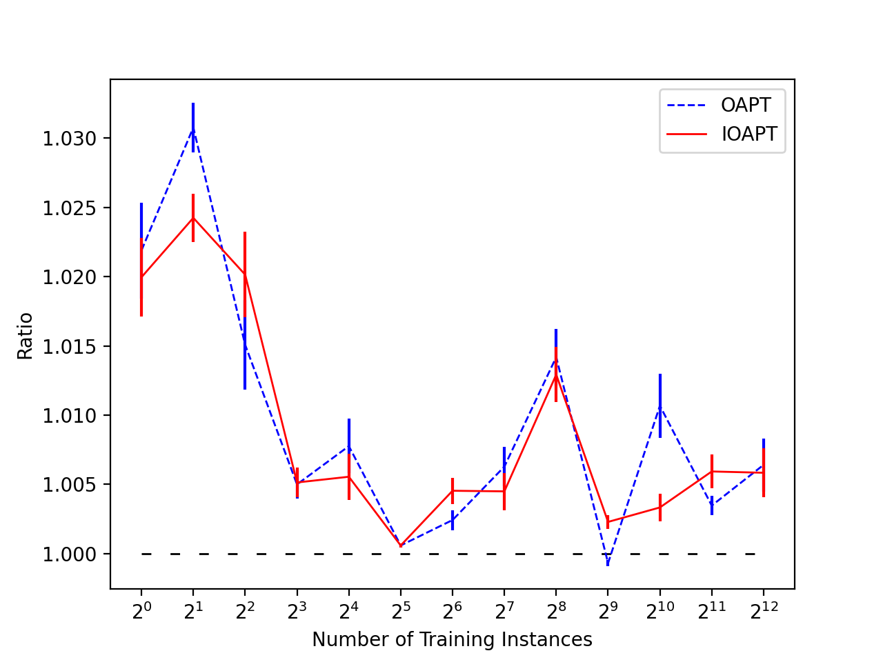
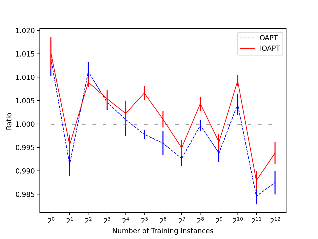


This section investigates the empirical performance of the proposed algorithm OAPT and IOAPT for the undirected Steiner tree problem. The goal is to answer the following two questions:
- •
Robustness - How much prediction accuracy does the algorithms need to outperform the baseline algorithm empirically?
- •
Learnability - How many samples are required to empirically learn predictions sufficient for the algorithms to perform better than the baseline?
The baseline we compare against is the online greedy algorithm which is the best traditional online algorithm. We investigate the performance of both OAPT and IOAPT.
Setup
The experiments33 3 The code is available at https://github.com/Chenyang-1995/Online-Steiner-Tree are conducted on a machine running Ubuntu 18.04 with an i7-7800X CPU and 48 GB memory. Experiments are averaged over 10 runs. We consider two types of graphs.
Random Graphs.
The number of nodes in a graph is set to be 2,000 and 50,000 edges are selected uniformly at random. The cost of each edge is an integer sampled uniformly from . To ensure the connectivity of graphs, we add all remaining edges to form a complete graph, given the edges high cost of 100,000.
Road Graphs.
The road network of Bay Area is provided by The 9th DIMACS Implementation Challenge44 4 http://users.diag.uniroma1.it/challenge9/download.shtml in graph format where a node denotes a point in Bay Area and the cost of an edge is the road length between the two endpoints. The original data contains 321,270 nodes and 400,086 edges. In the experiments, we employ the same sampling method as in (Moseley, Vassilvitskii, and Wang 2021) to sample connected subgraphs from this large graph. Briefly, we draw rectangles with a certain size on the road network randomly and construct a subgraph from each rectangle. The experiments employ 4 sampled subgraphs with nodes and edges. These graphs give the same trends, thus, we show one such graph in the main body and others appear Appendix .
The terminal set and the prediction are constructed differently depending on the experiments.
Robustness to Accuracy
This experiment tests the performance of OAPT and IOAPT when the prediction accuracy varies. Recall that is the number of terminals. We set and respectively for random graphs and road graphs unless stated otherwise55 5 We also conduct experiments with different numbers of terminals. The results are present in Appendix C.. The set of terminals are sampled uniformly from the vertex set . They arrive in random order.
We now construct the predictions. Let be a parameter corresponding to the prediction accuracy. First, we sample a node set with nodes uniformly from the terminal set . And then another node set with nodes is sampled uniformly from the non-terminal nodes . Let be the predicted terminal set . Notice that indicates the prediction accuracy. Thus, testing the performance of algorithms with different ’s answers the robustness question. This experiment is in Fig. 2 and 3.
Learning the Terminals
Here we construct instances where the algorithm explicitly learns the terminals. Each such instance will have a distribution over terminal sets of size and employ random order. We will sample training instances of terminals . The learning algorithm used to predict terminals is defined as follows.
The Learning Algorithm.
A node is predicted to be in with probability if , where is the number of sampled sets in which node appears and is a parameter in . Note that the number of predicted terminals may not equal .
There is a question on how to choose . This is done as follows. We choose an instance from the training set at random and check which would give OAPT (IOAPT) the best performance on this instance. We then use this for OAPT (IOAPT) on the online instance. For efficiency, we only consider .
Distribution for Random Graphs.
Two distributions are considered for random graphs. The first is a bad distribution where there is nothing to learn, the uniform distribution. In this case, all terminals are drawn uniformly from . The second is called a two-class distribution where there is a set of nodes to learn. Let be a small collection of nodes that will be terminals with higher probability. is set to nodes uniformly at random. Let be the number of terminals. Half are drawn from and half from . Here we hope the learning algorithm quickly learns , and further, our algorithms can take advantage of the predictions. The results appear in Fig. 2 and 2.
Distribution for Road Graphs.
This experiment is designed to model the case where terminals can appear in geographical similar locations. The graph will be clustered and a specified number of terminals will arrive per cluster following a distribution over nodes in the cluster. Use to denote the radius of the graph. Given a parameter , partition all nodes into several clusters such that the radius of each cluster is at most . The greedy clustering algorithm (Gonzalez 1985) is used and described in Appendix A. We let in the experiments unless state otherwise. The terminal set is obtained by picking random clusters and sampling terminals uniformly from each selected cluster. We let be 10 and 100. When the distribution is harder to learn than when . See Fig. 3 and 3 for the results.
Empirical Discussion
We see the following trends.
- •
- •
Fig. 2 3 show the algorithms are robust for difficult distributions, which are sparse distributions where there is effectively nothing to learn. The learning algorithm will quickly realize that predictions cause negative effects and then output very few predicted terminals (see prediction errors in Appendix C for more corroborating experiments). After tens of training instances, the ratios become never worse than 1.01.
- •
Fig. 2 3 show the learning algorithm quickly learns good distributions. Further, both online algorithms have strong performance using the predictions. We conclude that with a small number of training samples, the learning algorithm is able to learn useful predictions sufficient for the online algorithms to outperform the baseline.
These experiments corroborate the theory. The algorithms obtain much better performance than the baseline even with modestly good predictions. If given very inaccurate predictions, the algorithms are barely worse than the baseline. Moreover, we see that only a small number of sample instances are needed for the algorithms to have competitive performance when terminals arrive from a good distribution.
5 Conclusion
Online Steiner tree is one of the most fundamental online network design problems. It is a special case or a sub-problem of many online network design problems. Steiner tree captures the challenge of building networks online and, moreover, Steiner tree algorithms are often used as building blocks or subroutines for more general problems. As the community expands the learning augmented algorithms area into more general online network design problems, this paper provides models, and algorithmic and analysis techniques that can be leveraged for these problems.
Acknowledgements
Chenyang Xu was supported in part by Science and Technology Innovation 2030 –”The Next Generation of Artificial Intelligence” Major Project No.2018AAA0100902. Benjamin Moseley was supported in part by NSF grants CCF-1824303, CCF-1845146, CCF-2121744, CCF-1733873 and CMMI-1938909. Benjamin Moseley was additionally supported in part by a Google Research Award, an Infor Research Award, and a Carnegie Bosch Junior Faculty Chair. We thank Yuyan Wang for sharing their experimental data and thank the anonymous reviewers for their insightful comments and suggestions. Further, we thank Mirko Giacchini for the discussion on some implementation details of the proposed algorithms.
References
- Anand, Ge, and Panigrahi (2020) Anand, K.; Ge, R.; and Panigrahi, D. 2020. Customizing ML Predictions For Online Algorithms. ICML 2020.
- Angelopoulos (2008) Angelopoulos, S. 2008. A Near-Tight Bound for the Online Steiner Tree Problem in Graphs of Bounded Asymmetry. In Algorithms - ESA 2008, 16th Annual European Symposium, Karlsruhe, Germany, September 15-17, 2008. Proceedings, 76–87.
- Angelopoulos (2009) Angelopoulos, S. 2009. Parameterized Analysis of Online Steiner Tree Problems. In Adaptive, Output Sensitive, Online and Parameterized Algorithms, 19.04. - 24.04.2009.
- Antoniadis et al. (2020a) Antoniadis, A.; Coester, C.; Eliás, M.; Polak, A.; and Simon, B. 2020a. Online metric algorithms with untrusted predictions. CoRR, abs/2003.02144.
- Antoniadis et al. (2020b) Antoniadis, A.; Gouleakis, T.; Kleer, P.; and Kolev, P. 2020b. Secretary and Online Matching Problems with Machine Learned Advice. In Advances in Neural Information Processing Systems 33: Annual Conference on Neural Information Processing Systems 2020, NeurIPS 2020, December 6-12, 2020, virtual.
- Bachhiesl et al. (2002) Bachhiesl, P.; Paulus, G.; Prossegger, M.; Werner, J.; and Stögner, H. 2002. Cost Optimized Layout of Fibre Optic Networks in the Access Net Domain. In Operations Research Proceedings 2002, Selected Papers of the International Conference on Operations Research (SOR 2002), Klagenfurt, Austria, September 2-5, 2002, 247–252.
- Balcan et al. (2018) Balcan, M.; Dick, T.; Sandholm, T.; and Vitercik, E. 2018. Learning to Branch. In Dy, J. G.; and Krause, A., eds., Proceedings of the 35th International Conference on Machine Learning, ICML 2018, Stockholmsmässan, Stockholm, Sweden, July 10-15, 2018, volume 80 of Proceedings of Machine Learning Research, 353–362. PMLR.
- Balcan, Dick, and White (2018) Balcan, M.; Dick, T.; and White, C. 2018. Data-Driven Clustering via Parameterized Lloyd’s Families. In Bengio, S.; Wallach, H. M.; Larochelle, H.; Grauman, K.; Cesa-Bianchi, N.; and Garnett, R., eds., Advances in Neural Information Processing Systems 31: Annual Conference on Neural Information Processing Systems 2018, NeurIPS 2018, 3-8 December 2018, Montréal, Canada, 10664–10674.
- Bamas et al. (2020) Bamas, É.; Maggiori, A.; Rohwedder, L.; and Svensson, O. 2020. Learning Augmented Energy Minimization via Speed Scaling. In Larochelle, H.; Ranzato, M.; Hadsell, R.; Balcan, M.; and Lin, H., eds., Advances in Neural Information Processing Systems 33: Annual Conference on Neural Information Processing Systems 2020, NeurIPS 2020, December 6-12, 2020, virtual.
- Bamas, Maggiori, and Svensson (2020) Bamas, É.; Maggiori, A.; and Svensson, O. 2020. The Primal-Dual method for Learning Augmented Algorithms. In Advances in Neural Information Processing Systems 33: Annual Conference on Neural Information Processing Systems 2020, NeurIPS 2020, December 6-12, 2020, virtual.
- Berman and Coulston (1997) Berman, P.; and Coulston, C. 1997. On-line algorithms for Steiner tree problems. Conference Proceedings of the Annual ACM Symposium on Theory of Computing, 344–353. Proceedings of the 1997 29th Annual ACM Symposium on Theory of Computing ; Conference date: 04-05-1997 Through 06-05-1997.
- Bhaskara et al. (2020) Bhaskara, A.; Cutkosky, A.; Kumar, R.; and Purohit, M. 2020. Online Learning with Imperfect Hints. CoRR, abs/2002.04726.
- Byrka et al. (2010) Byrka, J.; Grandoni, F.; Rothvoß, T.; and Sanità, L. 2010. An improved LP-based approximation for steiner tree. In Proceedings of the 42nd ACM Symposium on Theory of Computing, STOC 2010, Cambridge, Massachusetts, USA, 5-8 June 2010, 583–592.
- Chawla et al. (2020) Chawla, S.; Gergatsouli, E.; Teng, Y.; Tzamos, C.; and Zhang, R. 2020. Pandora’s Box with Correlations: Learning and Approximation. arXiv:1911.01632.
- Chiang et al. (2013) Chiang, M.; Lam, H.; Liu, Z.; and Poor, H. V. 2013. Why Steiner-tree type algorithms work for community detection. In Proceedings of the Sixteenth International Conference on Artificial Intelligence and Statistics, AISTATS 2013, Scottsdale, AZ, USA, April 29 - May 1, 2013, 187–195.
- Dinur and Steurer (2014) Dinur, I.; and Steurer, D. 2014. Analytical approach to parallel repetition. In Shmoys, D. B., ed., Symposium on Theory of Computing, STOC 2014, New York, NY, USA, May 31 - June 03, 2014, 624–633. ACM.
- Gollapudi and Panigrahi (2019) Gollapudi, S.; and Panigrahi, D. 2019. Online Algorithms for Rent-Or-Buy with Expert Advice. In Chaudhuri, K.; and Salakhutdinov, R., eds., Proceedings of the 36th International Conference on Machine Learning, ICML 2019, 9-15 June 2019, Long Beach, California, USA, volume 97 of Proceedings of Machine Learning Research, 2319–2327. PMLR.
- Gonzalez (1985) Gonzalez, T. F. 1985. Clustering to Minimize the Maximum Intercluster Distance. Theor. Comput. Sci., 38: 293–306.
- Gupta, Hajiaghayi, and Kumar (2007) Gupta, A.; Hajiaghayi, M.; and Kumar, A. 2007. Stochastic Steiner Tree with Non-uniform Inflation. In Approximation, Randomization, and Combinatorial Optimization. Algorithms and Techniques, 10th International Workshop, APPROX 2007, and 11th International Workshop, RANDOM 2007, Princeton, NJ, USA, August 20-22, 2007, Proceedings, 134–148.
- Gupta and Pál (2005) Gupta, A.; and Pál, M. 2005. Stochastic Steiner Trees Without a Root. In Automata, Languages and Programming, 32nd International Colloquium, ICALP 2005, Lisbon, Portugal, July 11-15, 2005, Proceedings, 1051–1063.
- Gupta and Roughgarden (2017) Gupta, R.; and Roughgarden, T. 2017. A PAC Approach to Application-Specific Algorithm Selection. SIAM J. Comput., 46(3): 992–1017.
- Im et al. (2021) Im, S.; Kumar, R.; Qaem, M. M.; and Purohit, M. 2021. Non-Clairvoyant Scheduling with Predictions. In Agrawal, K.; and Azar, Y., eds., SPAA ’21: 33rd ACM Symposium on Parallelism in Algorithms and Architectures, Virtual Event, USA, 6-8 July, 2021, 285–294. ACM.
- Imase and Waxman (1991) Imase, M.; and Waxman, B. M. 1991. Dynamic Steiner Tree Problem. SIAM J. Discret. Math., 4(3): 369–384.
- Indyk et al. (2020) Indyk, P.; Mallmann-Trenn, F.; Mitrovic, S.; and Rubinfeld, R. 2020. Online Page Migration with ML Advice. CoRR, abs/2006.05028.
- Jiang, Panigrahi, and Sun (2020) Jiang, Z.; Panigrahi, D.; and Sun, K. 2020. Online Algorithms for Weighted Paging with Predictions. In Czumaj, A.; Dawar, A.; and Merelli, E., eds., 47th International Colloquium on Automata, Languages, and Programming, ICALP 2020, July 8-11, 2020, Saarbrücken, Germany (Virtual Conference), volume 168 of LIPIcs, 69:1–69:18. Schloss Dagstuhl - Leibniz-Zentrum für Informatik.
- Karp (1972) Karp, R. M. 1972. Reducibility Among Combinatorial Problems. In Proceedings of a symposium on the Complexity of Computer Computations, held March 20-22, 1972, at the IBM Thomas J. Watson Research Center, Yorktown Heights, New York, USA, 85–103.
- Kou, Markowsky, and Berman (1981) Kou, L. T.; Markowsky, G.; and Berman, L. 1981. A Fast Algorithm for Steiner Trees. Acta Informatica, 15: 141–145.
- Kraska et al. (2018) Kraska, T.; Beutel, A.; Chi, E. H.; Dean, J.; and Polyzotis, N. 2018. The Case for Learned Index Structures. In Proceedings of the 2018 International Conference on Management of Data, SIGMOD ’18, 489–504. New York, NY, USA: ACM. ISBN 978-1-4503-4703-7.
- Kurz, Mutzel, and Zey (2012) Kurz, D.; Mutzel, P.; and Zey, B. 2012. Parameterized Algorithms for Stochastic Steiner Tree Problems. In Mathematical and Engineering Methods in Computer Science, 8th International Doctoral Workshop, MEMICS 2012, Znojmo, Czech Republic, October 25-28, 2012, Revised Selected Papers, 143–154.
- Lappas et al. (2010) Lappas, T.; Terzi, E.; Gunopulos, D.; and Mannila, H. 2010. Finding effectors in social networks. In Proceedings of the 16th ACM SIGKDD International Conference on Knowledge Discovery and Data Mining, Washington, DC, USA, July 25-28, 2010, 1059–1068.
- Lattanzi et al. (2020) Lattanzi, S.; Lavastida, T.; Moseley, B.; and Vassilvitskii, S. 2020. Online Scheduling via Learned Weights. In Chawla, S., ed., Proceedings of the 2020 ACM-SIAM Symposium on Discrete Algorithms, SODA 2020, Salt Lake City, UT, USA, January 5-8, 2020, 1859–1877. SIAM.
- Lavastida et al. (2021) Lavastida, T.; Moseley, B.; Ravi, R.; and Xu, C. 2021. Learnable and Instance-Robust Predictions for Online Matching, Flows and Load Balancing. In Mutzel, P.; Pagh, R.; and Herman, G., eds., 29th Annual European Symposium on Algorithms, ESA 2021, September 6-8, 2021, Lisbon, Portugal (Virtual Conference), volume 204 of LIPIcs, 59:1–59:17. Schloss Dagstuhl - Leibniz-Zentrum für Informatik.
- Leitner et al. (2018) Leitner, M.; Ljubic, I.; Luipersbeck, M.; and Sinnl, M. 2018. Decomposition methods for the two-stage stochastic Steiner tree problem. Comput. Optim. Appl., 69(3): 713–752.
- Lykouris and Vassilvtiskii (2018) Lykouris, T.; and Vassilvtiskii, S. 2018. Competitive Caching with Machine Learned Advice. In Dy, J.; and Krause, A., eds., Proceedings of the 35th International Conference on Machine Learning, volume 80 of Proceedings of Machine Learning Research, 3302–3311. Stockholmsmässan, Stockholm Sweden: PMLR.
- Moseley, Vassilvitskii, and Wang (2021) Moseley, B.; Vassilvitskii, S.; and Wang, Y. 2021. Hierarchical Clustering in General Metric Spaces using Approximate Nearest Neighbors. In The 24th International Conference on Artificial Intelligence and Statistics, AISTATS 2021, April 13-15, 2021, Virtual Event, 2440–2448.
- Purohit, Svitkina, and Kumar (2018) Purohit, M.; Svitkina, Z.; and Kumar, R. 2018. Improving Online Algorithms via ML Predictions. In Advances in Neural Information Processing Systems 31: Annual Conference on Neural Information Processing Systems 2018, NeurIPS 2018, 3-8 December 2018, Montréal, Canada., 9684–9693.
- Rohatgi (2020) Rohatgi, D. 2020. Near-Optimal Bounds for Online Caching with Machine Learned Advice. In Chawla, S., ed., Proceedings of the 2020 ACM-SIAM Symposium on Discrete Algorithms, SODA 2020, Salt Lake City, UT, USA, January 5-8, 2020, 1834–1845. SIAM.
- Sadeghi and Fröhlich (2013) Sadeghi, A.; and Fröhlich, H. 2013. Steiner tree methods for optimal sub-network identification: an empirical study. BMC Bioinform., 14: 144.
- Schrijver (2003) Schrijver, A. 2003. Combinatorial optimization: polyhedra and efficiency, volume 24. Springer Science & Business Media.
- Takakashi (1980) Takakashi, H. 1980. An Approximate Solution for Steiner Problem in Graphs. Math. Japonica, 24(6): 573–577.
- Wei (2020) Wei, A. 2020. Better and Simpler Learning-Augmented Online Caching. CoRR, abs/2005.13716.
- Westbrook and Yan (1995) Westbrook, J. R.; and Yan, D. C. K. 1995. Linear Bounds for On-Line Steiner Problems. Inf. Process. Lett., 55(2): 59–63.
- Wu, Widmayer, and Wong (1986) Wu, Y.-F.; Widmayer, P.; and Wong, C.-K. 1986. A faster approximation algorithm for the Steiner problem in graphs. Acta informatica, 23(2): 223–229.
Appendix A Pseudo-codes for Algorithms
This section presents the pseudo-codes of algorithms mentioned in previous sections: algorithm OAPT, algorithm IOAPT, the algorithm for directed graphs, the learning algorithm and the clustering algorithm (a natural variant of the greedy algorithm given in (Gonzalez 1985)).
Appendix B Omitted Proofs
Proof of Lemma 5.
The proof follows by construction of an instance of online Steiner tree where OAPT has cost .
The instance is shown in Fig. 4. There is an edges of cost for . The edge has cost . There is a cycle where all edges have cost 1 except . Let the terminal set and the predicted terminal set . Thus, the prediction error . For the terminal set , we can easily find its optimal solution (illustrated by all solid edges in Fig. 4). That is the edges for . The cost of this solution is .
Consider OAPT. The algorithm first computes its minimum spanning tree, which is represented by dash edges in Fig. 4. This is the edges of the cycle . The cost of is .
Let the terminals arrive in the order of . When the second terminal arrives, algorithm OAPT finds is a terminal in and add the shortest path from to in , which is the path . The cost gained by this step is the cost of , i.e., . For each remaining terminal, algorithm OAPT adds the shortest edge with cost . Thus, the final cost of algorithm OAPT is ∎
Proof of Theorem 14.
The analysis of is easy. We know the shortest path from to is always no larger than OPT and the first case occurs times, thus
Now consider edges in . According to the definition of , the total cost of is at most . This is because a feasible solution can be obtained easily by choosing the shortest path for each terminal, whose objective value is at most .
When , the value of doubles at most times since according to the doubling condition. Each time doubles, a new tree is generated. Ideally, if we can bound each by a constant factor of OPT, can be bounded by .
Let be the smallest integer such that . The following summations are over the different powers of two that can take on.
∎
Now we state a theorem to show that our dependence of in the directed case is optimal.
Theorem 16.
For online directed Steiner tree with predicted terminals, given any , no online algorithm has a competitive ratio better than .
Proof of Theorem 12 and Theorem 16.
The two theorems share the same basic idea. Thus, we only take the undirected case for an example here.
Fix any . Let be a known hard online instance on terminals used to give the lower bound. Consider combining with terminals with cost edges. There are totally terminals. The zero-cost terminals arrive first and then the terminals arrive in adversarial order according to the hard instance .
No online algorithm can have a competitive ratio better than for this instance. Otherwise, such an algorithm would contradict the lower bound for undirected Steiner tree. ∎
Removing the assumption that .
Notice that if is far larger than , the error may not measure the quality of the prediction accurately. Thus, we redefine the prediction error when removing the assumption that . The analysis of our algorithms still holds given this new error. The number of terminals not in the prediction and the number of edges bought wrongly due to the prediction (e.g. the set in the undirected case) are still at most . This implies that the same competitive ratios can be obtained with effectively the same analysis. For the robustness of our algorithm, our proofs have shown that algorithm IOAPT and the directed case algorithm will never perform asymptotically worse than the best traditional algorithms no matter what the prediction is given. Thus, regardless of the definition of the error, their robustness ratios are always and , respectively.
Appendix C Additional Experimental Results
Robustness to Accuracy in Different Settings
This subsection shows the robustness performance of algorithms on random graphs under different ’s, , where is the number of terminals, and the performance on different road graphs fixing . From Fig. 5 and Fig. 6, they share roughly the same trend.


Prediction Errors in the Learning Experiments

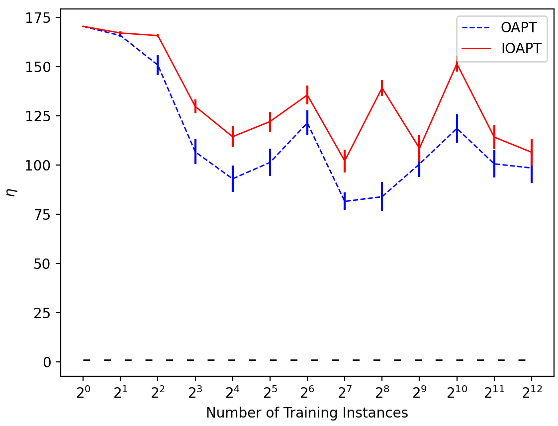


We present the prediction errors over different numbers of training instances. Noting that the number of predicted terminals may not equal , we define be the number of wrong predicted terminals here, i.e., . We see the following trends:
- •
For bad distributions (e.g. Fig. 7(a) 7(c)), the learning algorithm predicts almost no terminals after observing tens of instance, resulting in tiny in the figures. Recalling the performance shown in Section 4, when is small, the augmenting algorithms will switch to the greedy algorithm automatically and make the performance robust.
- •
For good distributions (e.g. Fig. 7(b) 7(d)), the learning algorithm quickly learns the nodes which become terminals with high probability. Although these predictions are still modestly accurate, they are sufficient for our algorithms to obtain comparable performance (recall Fig. 2 3 in the main body).