An augmented Lagrangian model for signal segmentation
Salvador Moll22footnotemark:
2
Department d’Anàlisi Matemàtica, Universitat de València
C/Dr. Moliner, 50, Burjassot, Spain
j.salvador.moll@uv.es
Vicent Pallardó
Universitat de València
C. Dr. Moliner, 50, Burjassot, Spain
vicentpallardojulia@gmail.com
Abstract. In this paper, we provide a new insight to the two–phase signal segmentation problem. We propose an augmented Lagrangian variational model based on Chan–Vese’s original one. By using both energy methods and PDE methods, we show, in the one dimensional case, that the set of minimizers to the proposed functional contains only binary functions and it coincides with the set of minimizers to Chan–Vese’s one. This fact allows us to obtain two important features of the minimizers as a byproduct of our analysis. First of all, for a piecewise constant initial signal, the jump set of any minimizer is a subset of the jump set of the given signal. Secondly, all of the jump points of the minimizer belong to the same level set of the signal, in a multivalued sense. This last property permits to design a trivial algorithm for computing the minimizers.
1 Introduction
Segmentation is the task of partitioning an object into its constituent parts. In signal or image processing, it consists in decomposing the domain of a given input: a signal (an interval in which case ) or an image () into some regions of interest. In the particular case of two–phase segmentation, the aim is to find an optimal partition into two disjoint subsets, the foreground domain and the background domain such that .
After the seminal work by Mumford and Shah [17], in which the authors introduced a celebrated variational model for image segmentation, Chan and Vese rewrote it in the two–phase framework [7]. They propose to obtain the optimal partition by minimizing the following energy functional
| (1.1) |
among all sets of finite perimeter and all constants , for some given parameters . From now on, we don’t distinguish between the weights of the foreground and background and thus we take . A minimizer can be considered as the foreground domain and as the background domain. In this case, the constants and turn out to be, the average of in and the average in , respectively. The authors proposed in [7] an iterative two step algorithm for finding the minimizers of the energy based on the level set formulation developed by Osher and Sethian [18]. Basically, after initialization of the constants, the first step consists in finding the corresponding minimizing set with fixed constants as a steady state solution of the correspondent - gradient flow of the functional associated to the level set formulation. Then, one recomputes the constants and cames back to the first step until convergence has been reached.
The main problem with this algorithm is that the energy functional is not convex. Therefore, the gradient descent scheme is prone to get stuck at critical points other than global minima. This issue was fixed by Chan- Esedoglou and Nikolova, who proved that minimizers to Chan-Vese’s level set functional with fixed constants (i.e. solutions to Step 2) are solutions to the following constraint convex energy minimization problem (and viceversa):
| (1.2) |
Observe that, if the solution is the characteristic function of a set with finite perimeter; , then, the energy in (1.2) coincides with that in (1.1). There are still two main problems: the main one remains at the nonconvex nature of the original energy functional; i.e. convergence of the algorithm to a global minima is not ensured, and it heavily depends on the initialization. Moreover, it is not known if Chan-Vese’s algorithm (with Chan-Esedoglu-Nikolova modification) could lead to non-binary solutions (see [9]).
The main objective of this work is to give another approach to original Chan-Vese’s minimizers in the easiest possible case, the one dimensional case, which corresponds to signal segmentation. In the context of signal sementation, Chan-Vese’s algortihm was already proposed in [8] and has been used in some works (see [15] or [16]). Our starting point is the functional appearing in Problem (1.2). We aim at minimizing, simultaneously the function and the constants . In order to do that, we introduce an augmented lagrangian version of the functional, coupled with the constraint . In this new functional, we replace the constants by BV functions while highly penalizing their variation. For any we define the functional by letting
| (1.3) |
where denotes the indicator function of the interval ; i.e.
The second term is implemented for penalizing the variation of the pair of functions . Observe that, letting we are forcing to become constants. With this addition, the functional fails to be convex. However, we can use standard PDE methods to obtain some features of the set of minimizers via its correspondent system of Euler-Lagrange equations. In particular, we prove the following results in the case that is an interval of :
Theorem 1.1.
Let . Then, if is a minimizer of , then are constants.
In order to characterize the first component of the minimizer we need to assume further that the datum is not too oscillatory in the following sense:
satisfies that for every ,
Observe that with this assumption we exclude some pathologies on the data such as having a fat Cantor set as a level set.
Theorem 1.2.
Given , for satisfying , any minimizer of is independent of and it satisfies that either is constant or ; i.e. is a binary function in .
With this last result, we can show that the set of minimizers of Chan-Vese’s problem (1.1) coincide with the set of minimizers of (independent of under the size condition above expressed). As a by-product of our analysis, we obtain two important properties of solutions to (1.1):
-
The jump set of any solution is concentrated in the topological boundary of a sole level set (in a multivalued sense, see (4.2) for the proper statement).
-
If is piecewise constant, then the jump set of any solution is contained in the jump set of .
These two properties, though quite intuitive in the one dimensional setting, were not known in the literature, to the best of our knowledge. Moreover, property allows to build a trivial algorithm to find the minimizers of Chan-Vese’s problem in the one-dimensional case.
The plan of the paper is the following one: In Section 2 we obtain the system of PDE’s that minimizers to satisfy; i.e. the corresponding Euler–Lagrange equations in this non-smooth case. In Section 3 we prove Theorems 1.1 and 1.2. Section 4 is devoted to the proof of properties and . In Section 4.2, we explain the trivial algorithm to compute the minimizers.We finish the paper with some conclusions and with an Appendix, in which we collect the existence of minimizers to as well as the proof of an auxiliary result we need.
Notations. Throughout the paper, denotes an open bounded set in with Lipschitz boundary and denotes the Lebesgue measure in . We denote by , the Lebesgue space of functions which are integrable with power with respect to . We use the notation to denote the scalar product between two functions. We denote by the Hilbert space and by the completion in of smooth functions with compact support in . We use standard notation for functions of bounded variation ( functions) as in [2]. In particular, given , we write , and for the absolutely continuous part of the measure with respect to , for the Cantor part of and for the jump part of , respectively. We use the notation for the left and right approximate limits of at (we use only this convention for the case of , ), for its jump set and will denote the Radon-Nikodym derivative of with respect to . Given a set we say that it is a set of finite perimeter in if , where denotes the characteristic function of the set . In this case, its perimeter is defined as . Finally, unless otherwise specified, we always identify a function (in or in ) by its precise representative.
2 System of Euler–Lagrange equations
In this Section, we derive the system of equations that minimizers of must satisfy. Although is not a convex functional in , it is a convex functional in each of their coordinates when one fixes the other two ones. Therefore, by standard results in convex analysis, we obtain that the Euler–Lagrange system of PDE’s is the following one:
| (2.1) |
where the symbol denotes the subdifferential (in ) of the following two extended real valued convex functions:
and
We easily note that a.e. , for any . Next result is crucial and permits to reformulate .
Theorem 2.1.
Let . Then,
Proof.
We point out that standard results to decompose the subdifferential of the sum, such as those in [6], cannot be applied since the interior of the domains of both functionals are empty. We follow the strategy of [19, Thm. 3.1], consisting in an ad-hoc proof by approximating the subdifferential of the indicator function by its Yoshida’s regularization. First of all, we state the following claim, whose proof we postpone to the Appendix.
Claim: Let be a Lipschitz non decreasing function. Then, it holds:
Since we know that the inclusion
is satisfied, it is sufficient to show the converse inclusion. Let be such that , and let . We define by
We note that is coercive, strictly convex and lower semi-continuous. Then, it is easy to see that is the unique minimizer of .
Now, for any , let be the Yoshida regularization of , i.e.
here subindexes represent respectively, the positive and the negative part of the function. We next consider defined by
where is a primitive of . We note that is coercive, strictly convex over and lower semi-continuous. Thus, has a unique minimizer which satisfies the corresponding Euler–Lagrange equation:
In consequence, we know that the following equation has a unique solution
Multiplying by both sides of the previous equation, we have, for any
Here, since for any , we note that . Moreover, by the previous Claim, we have that
Then, we see that and are bounded in and is bounded in and . Therefore, there is a sequence such that and there exists a function such that
Moreover, we can assume that there exist such that and converge weakly in to and , respectively.
In addition, we note that
for any and thus, we have
Hence, we can show that a.e. in . We conclude that
This implies that is a minimizer of . Then, , and consequently, in , which finishes the proof. ∎
Up to this point, we have worked without imposing any restriction in the dimension of the domain, Now, we introduce the characterization of the subdifferential of the total variation in , proposed by Andreu, Ballester, Caselles and Mazón in [3] (see also [4]), in the specific case of the domain being an interval in 1-D, which we take as without loose of generality, (see [10] for a proof).
Theorem 2.2 (TV characterization in 1D).
Let be in such that . Then if and only if there exists such that a.e. and
where the measure is defined as
for any Borel set .
With this characterization in mind, the system of Euler–Lagrange equations can be rephrased in the following way:
Proposition 2.3.
Let be a minimizer of . Then, there exist , ,, corresponding to , and , respectively as given by Theorem 2.2, and such that
| (2.2) |
3 Proofs of the main results
3.1 Proof of Theorem 1.1
We need to show first the following auxiliary result.
Lemma 3.1 (Behaviour of ).
Let and , corresponding to as provided by Theorem 2.2. Then,
Proof.
We decompose both measures and in the following way:
Since both decompositions are mutually singular, we have
and thus, we have . ∎
Proof of Thm. 1.1.
Firstly, we note that if is a minimizer of , then, it is easy to see that all variables take values in a.e in as shown in Lemma A.1 in the Appendix. Suppose that there exists a Borel set such that . By Lemma 3.1, we know that there is such that , where is given by Proposition 2.3. Then, by , we have the next inequality
and in consequence, and thus, a contradiction by hypothesis.
In order to get that is also constant, we apply the same argument to . ∎
Under the size condition , which we assume from now on, we integrate the second and third Eqs. in (2.2) in and we obtain
| (3.1) |
in the case that is not constant with values or . If (resp. ) then (resp. ) can be any constant value in . We finally note that, being constants, the energy functional does not depend on . From now on, we will assume the size condition . We rename the constants as for consistency and remove the dependence by letting
3.2 Proof of Theorem 1.2
This Section is devoted to prove that the first coordinate of the minimizer is necessarily a binary BV function. Hereinafter, we assume that the datum satisfies . The proof will be done in two different steps. First of all, we show that if is a minimizer, then there is a “quasi–piecewise constant”competitor with lower energy than (or equal to) the corresponding to . Then, we prove that the competitor cannot be a minimizer in case it is not binary by using the PDE system (2.2).
We start by defining our concept of quasi–piecewise constant function.
Definition 3.2.
We say that is a quasi–piecewise constant if there exists a piecewise constant function and an a.e binary function which fulfill that they are not non-0 simultaneously and
Theorem 3.3.
Let . Given a minimizer of , there exists a quasi–piecewise constant satisfying
| (3.2) |
Proof.
Let be in such that and , and let be the vector field associated to as given by Theorem 2.2. We distinguish two cases:
- 1.
The case : We assume without loss of generality that (for , the argument is analogous). Under this assumption, we know that is continuous at (remember that we always identify a BV function with its precise representative) and thus, in a neighbourhood of denoted by . Hence, using , we know that
(3.3) Since , we have by the above expression that and thus, its lateral traces and are well defined. In addition, since and , this implies that
and we have, by (3.3) that
Then, we note that the set
is a subset of the following set: We note that where and are the (topological) interior and boundary of , respectively. Particularly, we note that
where is a disjoint collection of open intervals; and by assumption on and the fact that .
Next, we will modify in each interval to decrease the energy. Before doing it, we point out that, for fixed, minimizing is equivalent to minimize
Since , we observe that
Therefore, if we take it is easy to show that
- 2.
If : Since , we take the largest interval containing such that . By Lemma 3.1, in this interval and thus, is constant in .
Consequently, we note that can be decomposed as:
such that is a subset of
Defining
we obtain that the inequality (3.2) is clearly satisfied. Note that is a piecewise constant function in because of the reasoning in (i) and (ii) and thus, we can take
Finally, as and are disjoint, we obtain that is a quasi–piecewise constant function. ∎
We introduce now two useful remarks:
Remark 3.4.
Let be a minimizer of such that . Defining , it is easy to show that , and that . On account of it, we assume hereinafter that . Furthermore, if , we note that
and thus, in order to be a minimizer, is a necessarily a constant function.
Remark 3.5.
Let be a minimizer of and suppose that there exist such that , , , for any . By integrating on , we have that
where corresponds to . Note that the right hand side term is equal to , or because of the fact that in the jump set as a consequence of Lemma 3.1; as , if , then
- •
when jumps toward a lower step in .
- •
when jumps toward an upper step in .
After these remarks, we prove the following statement:
Proposition 3.6.
Let be a minimizer of such that is a quasi–piecewise constant function. Then either is constant or is an a.e. binary function.
Proof.
This statement is proved by contradiction. We suppose that is not an a.e binary function and not constant, i.e, has some non-binary step ( being the piecewise constant part). Let be such that . In addition, let and . According to the relation , there are three different cases to study:
- 1.
(or , resp.): We define
where (or , resp.). In any case, according to Remarks 3.4 and 3.5, we can suppose that and
Since , we obtain
It is clear that . Then, is a minimizer too. Consequently, by (3.1), we have
i.e. where we denoted by , and . Then,
Since and , we have This yields
thus leading to , i.e, to a contradiction by Remark 3.4.
- 2.
(or , resp.): Similarly as before, we consider
where (or , resp.). In any case, according to Remarks 3.4 and 3.5, we can suppose that and
We observe that
where and are the constants defined in the previous case and . Then, it is easy to check that . Again, is a minimizer and thus, it satisfies (3.1). Repeating the reasoning in the previous case (replacing instead of ), we obtain
and if we redo the same computations for we obtain the same equation, thus leading to , i.e, to a contradiction as before.
- 3.
(or , resp.): In this case, we define
where (or , resp.). Once again, repeating the computations in the previous case, we end up with , thus finishing the proof.
∎
4 Properties of minimizers
4.1 Proof of Properties and
In this Section, we show that the set of minimizers of coincides with that of minimizers to Chan-Vese and we prove Properties and of the minimizers.
Remark 4.1.
It is obvious that, given of finite perimeter,
Then, we note that
| (4.1) | |||||
On the other hand, by Theorem 1.2, we now that the minimum of is achieved in a constant or binary BV function , for the first coordinate. Then, (or )for a set of finite perimeter, which proves the reverse inequality in (4.1). This shows that minimizers of coincide with Chan-Vese’s minimizers.
We now prove Properties and :
Suppose that and that , . Then, as explained in Remark 3.5, , with corresponding to as given by Theorem 2.2. Moreover, since , by , as in the Proof of Theorem 3.3 that
If instead , , one gets
Therefore
| (4.2) |
where the image of a jump point is understood in a multivalued sense (i.e. ). Note that this fact almost proves Properties and . The only remaining thing to prove is that a jump point cannot exist in the interior of . Suppose, by contradiction that and let be such that . Without loosing generality, we can suppose that in and that . Then, considering , we easily get that and, therefore, is a minimizer too. Then, repeating the reasoning in Proposition 3.6, in case we arrive at a contradiction, which finishes the proof of Properties and .
Remark 4.2.
We note that Properties and of the minimizers are only expected to hold in the one–dimensional case. In fact, an easy counterexample in two dimensions is provided by with and . In this case is precisely the boundary of the square while it can be proved that, for any Chan-Vese’s minimizer cannot be either or , thus showing that and do not hold.
In fact, Chan-Vese’s energy for these two candidates is exactly (for , ) and (for , , ). Therefore, for , is not a minimizer. On the other hand, it is easy to modify the corners of the square by reducing the perimeter and not changing to much the fidelity term in the energy. We modify , calling the new set , by removing the corners through the use of -radius circumferential arches tangent to every two contiguous sides of . (see Fig. 2). Then one can check that , , for satisfying
has strictly less energy. This fact is related to the non-calibrability of the set with respect to the isotropic norm in the total variation (see [1]).


Therefore, if one wants to obtain similar results to Properties and in higher dimensions, the total variation term needs to be changed by an anisotropic version of it as in the case of the anisotropic Rudin–Osher–Fatemi functional, for which stability of piecewise constant functions on rectangles has been recently shown in [14] and [13]. We will investigate this issue further in a subsequent paper.
4.2 Application of the properties
In this Section, we propose a trivial way to approach the solution of the 1D Chan-Vese problem by using properties and of the minimizer. We will also comment on the pros of this trivial algorithm in front of those based on a Gradient Descent (GD) scheme. We remark that those algorithms are applied in an 1-D version of alternating scheme proposed by Chan and Vese in [7]. Hereinafter, we will assume that the boundary of each level of the datum set has a finite number of points.
We start with the general case. In this one, the idea is:
- (1)
Take a discretization of the range, thus defining the working level sets.
- (2)
In each level set, compute the binary candidate with the least energy with jumps in the boundary of the level set.
- (3)
Compare between the solutions and choose one with the smallest energy.
Besides, in the case of being a step function, we can further simplify the previous idea thanks to the implementation of the inclusion . This reduction is based on trying all the possible combinations of characteristic solutions whose jump set is a subset of .
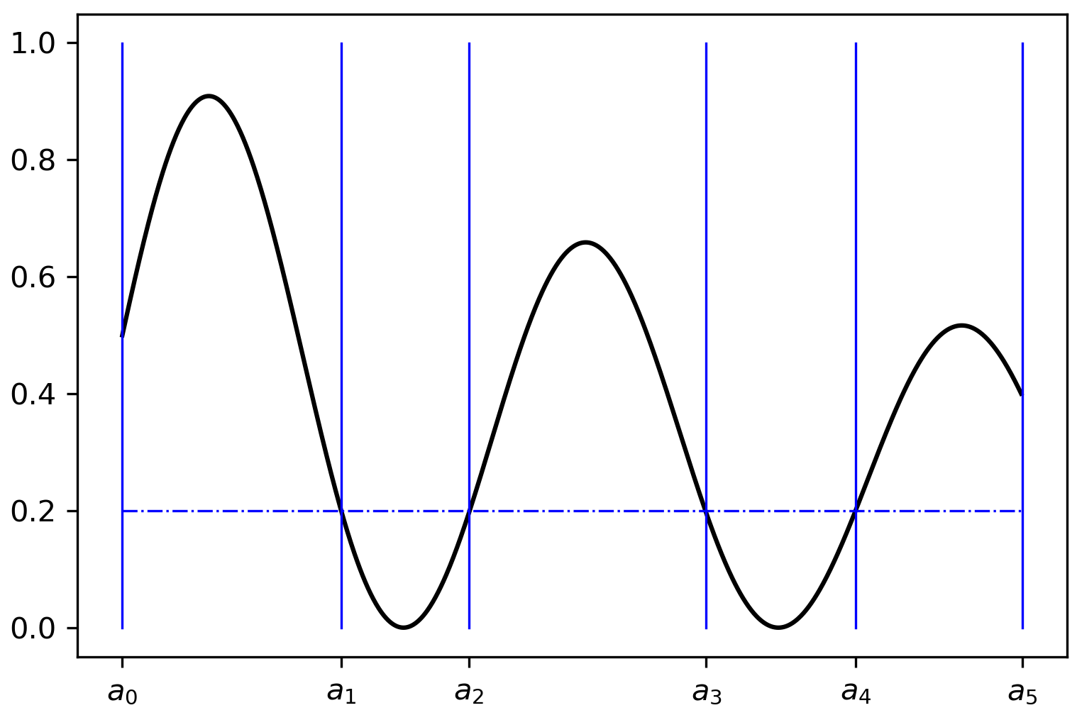
In Figure 3, we sketch how to perform Step 2 in the general algorithm for a fixed level set. Firstly, we obtain all possible jump points for the possible minimizer , (). Then, we know that the candidate to minimizer takes the form
Computing all the possibilities we keep the candidate with the least energy among them. We compare its energy with that of the candidate obtained from a previous bigger level set and the procedure is repeated until we reach the lowest level set in the discretization. To show the suitability of this trivial approach in some situations, we present the following example:
Example 1.
Suppose we segment by the 1-D Chan-Vese model a signal whose shape is similar to the one of the Weierstrass function. This kind of signals has the property of exhibiting abrupt variations of its slope on the whole domain, which causes problems for GD based algorithms. This intuitive idea can be seen in Figure 4, where we compute an approximation to the minimizer using two different approaches: in one of them we use the alternating Chan-Vese scheme with a GD-based method (ADAGRAD algorithm, see [11]); while on the other one we use the trivial scheme explained above.


We note how the GD based approach suffers from the variations of the signal, thus affecting to the performance of the alternating Chan-Vese scheme. In contrast, the trivial approach, based on properties and , provides an adequate minimizer approximation. Moreover, we note that even if we chose a particular case of an algorithm based on GD, this type of behaviour is a trend in any of these algorithms. Therefore, the use of the scheme presented in this paper is beneficial in situations where the application of GD (or variants) gives a wrong segmentation of the signal, as shown in the figure above.
Appendix A Appendix
In this Appendix, we show that the functional always has a minimizer regardless of the dimension of the domain. Note that, for , in the –dimensional case, according to Remark 3, existence of minimizers follows directly from existence of minimizers to Chan-Vese’s functional. Here, we give a direct proof for any , which, in turn, provides an alternative proof of existence of solutions to (1.1). Existence of minimizers will be shown through the study of the following auxiliary energy: ,
Existence of minimizers to functional is guaranteed by the Direct Method in the Calculus of Variations since the functional is easily seen to be lower semicontinuous in and coercive. Now, we relate both functionals and in the following result:
Lemma A.1.
Let . Then,
| (A.1) |
where is the truncation function in ; i.e. .
Proof.
Firstly note that we can suppose that a.e. (otherwise, both terms in the inequality are equal to ). Now, we observe that the following inequality is easily seen to be true (since ):
In consequence,
| (A.2) |
Moreover, applying the Chain Rule in the composition of a function and a Lipschitz function ([2, Theorem 101]), we have
Proposition A.2.
For any , the functional has a minimizer .
Proof.
The proof follows directly from Lemma A.1 since we obtain that
Therefore, by the existence of minimizers to we can conclude that admits (at least) one minimizer (which moreover belongs to ). ∎
We finish this Appendix with the proof of the
Claim: Let be a Lipschitz non decreasing function. Then, the following equality holds:
Proof.
Since this Claim is stated in the multidimensional case, we need to recall (see [3]) that if, and only if, there exists a vector field with , such that , and
with being the Radon measure defined by (see [5] for precise definitions and results here stated)
being the Radon–Nikodym derivative of over and being the weak normal trace of on the boundary. Note that this implies, in particular, that
| (A.4) |
Since is Lipschitz, by Chain’s rule, we have that . Suppose now that and is increasing. By [5, Proposition 2.8], we have that , -a.e. Observe that in this case, the measure is absolutely continuous with respect to and vice versa. Then, a property holds -a.e. iff it holds a.e. Therefore by integration by parts (see [5]), we obtain
| (A.5) | |||||
In the general case, we approximate by a sequence of increasing functions , being a symmetric mollifier. Therefore, it is easy to check that strictly converges to and we finish the proof by using (A.5). ∎
References
- [1] Alter, F., Caselles, V. and Chambolle, A., A characterization of convex calibrable sets in , Mathematische Annalen, 332, pp. 329–366, 2005.
- [2] Ambrosio, L., Fusco, N. and Pallara, D., Functions of Bounded Variation and Free Discontinuity Problems. Oxford Mathematical Monographs, 2000.
- [3] Andreu, F., Ballester, C., Caselles, V. and Mazón, J.M., Minimizing total variation flow. Differential Integral Equations, 14(3), pp. 321-360, 2001.
- [4] Andreu, F., Caselles, V. and Mazón, J.M., Parabolic Quasilinear Equations Minimizing Linear Growth Functionals, Progress in Mathematics, 223, Birkhäuser Verlag, Basel, 2004,
- [5] Anzellotti, G., Pairings between measures and bounded functionsand compensated compactness. Annali di Matematica Pura et Applicata, 135, pp. 293–318, 1983.
- [6] Brezis, H., Opérateurs maximaux monotones et semigroupes de contractions dans les espace de Hilbert. North-Holland Publishing Company, 1973.
- [7] Chan, T., and Vese, L., Active contours without edges. IEEE Transactions on image processing, 10(2), pp. 130–141, 2001.
- [8] Chan, T. and Vese, L. A Multiphase Levet Set Framework for Image Segmentation Using the Mumford and Shah Model International Journal of Computer Vision, 50, pp. 271-293, 2002.
- [9] Chan, T., Esedoglu, S. and Nikolova, M., Algorithms for finding global minimizers of image segmentation and denoising models. SIAM Journal on Applied Mathematics, 66(5), pp. 1632–1648, 2006.
- [10] Crasta, G. and De Cicco, V., Anzellotti’s pairing theory and the Gauss-Green theorem, Advances in Mathematics, 343, pp. 935–970, 2019
- [11] Duchi, J., Hazan, E. and Singer, Y., Adaptive Subgradient Methods for Online Learning and Stochastic Optimization Journal of Machine Learning Research, 12, pp. 2121–2159, 2011.
- [12] Evans, L. C. and Gariepy, R. F., Measure theory and fine properties of functions, CRC Press, 1992
- [13] C. Kirisits, C., Scherzer, O. and Setterqvist, E., Preservation of Piecewise Constancy under TV Regularization with Rectilinear Anisotropy, in Scale Space and Variational Methods in Computer Vision , Lecture Notes in Computer Science vol. 11603, Springer , pp 510–521, 2019.
- [14] Łasica, M, Moll, S. and Mucha, P., Total Variation Denoising in Anisotropy, SIAM J. Imaging Sci, 10(4), pp.1691–1723, 2017
- [15] Mahmoodi, S. and Sharif, B.S., Signal Segmentation and denoising algorithm based on energy optimisation. Signal Processing, 85(6), pp. 1845-1851, 2005.
- [16] Mahmoodi, S. and Sharif, B.S., A nonlinear variational method for signal segmentation and reconstruction using level set algorithm, Signal Processing, 86(11), pp. 3496–3504, 2006.
- [17] Mumford, D. and Shah, J., Optimal approximation by piecewise smoothfunctions and associated variational problems. Commum. Pure Applied Mathematics, 42(5), pp. 577-685, 1989.
- [18] Osher, S. and Sethian, J. A., Fronts propagating with curvature-dependent speed: Algorithms based on Hamilton–Jacobi Formulation. Journal of Computational Physics, 79(1), pp. 12-49, 1988.
- [19] Shirakawa, K. and Kimura, M., Stability analysis for Allen–-Cahn type equation associated with the total variation energy. Nonlineal Analysis: Theory, Methods and Applications, 60(2), pp. 257-282, 2005.