A Novel Tropical Geometry-based Interpretable Machine Learning Method: Application in Prognosis of Advanced Heart Failure
Abstract
A model’s interpretability is essential to many practical applications such as clinical decision support systems. In this paper, a novel interpretable machine learning method is presented, which can model the relationship between input variables and responses in humanly understandable rules. The method is built by applying tropical geometry to fuzzy inference systems, wherein variable encoding functions and salient rules can be discovered by supervised learning. Experiments using synthetic datasets were conducted to investigate the performance and capacity of the proposed algorithm in classification and rule discovery. Furthermore, the proposed method was applied to a clinical application that identified heart failure patients that would benefit from advanced therapies such as heart transplant or durable mechanical circulatory support. Experimental results show that the proposed network achieved great performance on the classification tasks. In addition to learning humanly understandable rules from the dataset, existing fuzzy domain knowledge can be easily transferred into the network and used to facilitate model training. From our results, the proposed model and the ability of learning existing domain knowledge can significantly improve the model generalizability. The characteristics of the proposed network make it promising in applications requiring model reliability and justification.
Index Terms:
Interpretable Machine Learning, Explainable Machine Learning, Artificial IntelligenceI INTRODUCTION
Heart failure (HF) afflicts 6.5 million Americans 20 and older, with its prevalence projected to increase annually [1, 2]. Treatment of these patients remains limited both by medical therapies and by organ availability. The appropriate delivery of advanced therapies, heart transplantation (HT) or mechanical circulatory support (MCS) implantation, to patients with end-stage HF is highly nuanced and requires expertise from advanced HF cardiologists. Due to the high prevalence of HF, the majority of patients are managed by primary care physicians or cardiologists, who lack training in the management of these patients. Thus, there is a need for artificial intelligence (AI) based tools that can systematically identify patients warranting referral to an advanced HF cardiologist for consideration of HT or MCS implantation. In this study, we aims to build a clinical decision-making model that can differentiate patients eligible for and most likely to benefit from advanced therapies; such as durable MCS or HT; from those too well, too sick, or otherwise ineligible for advanced therapies.
AI and machine learning (ML) have been increasingly applied to healthcare problems [3]. Previous studies investigated AI in disease diagnosis, treatment effectiveness prediction, and patient outcome prediction [4, 5, 6, 7]. Several studies have shown that AI performs as well as or better than humans [8]. With a lower cost, AI-based decision support systems have the potential to improve patient management.
Despite tremendous progress in the field of AI/ML-based clinical decision support systems, there are still significant challenges that prevent widespread use of these methods in sensitive applications. While traditional models such as linear models and decision trees provide accessible reasoning, they are less capable of achieving high performance on complicated clinical problems. In contrast, a wide spectrum of ML models with higher complexity, including families of neural networks and support vector machines (SVM), can yield good metrics on experimental datasets. However, these “black box” models lack transparency and justification of their recommendations, making them much less likely to be trusted in clinical applications. Moreover, many popular ML methods, such as deep learning, utilize a large number of parameters, thus requiring large training datasets to avoid overfitting the data. However, in many clinical applications, collecting large annotated training datasets may be costly or even impossible. As such, there is a clear need for an interpretable ML model that can reliably model data using relatively small training sets. In addition, in healthcare applications, there exist many invaluable heuristics derived from domain knowledge expertise, often in the form of approximate rules that are used by human experts. For example, when caring for patients with end-stage HF, cardiologists use their clinical intuitions, paired with transplant guidelines, to identify patients who may benefit from a durable MCS device or HT. In the majority of existing AI/ML models, there is no clear mechanism to leverage such approximate knowledge for model formation or training.
The motivation of this study is to solve the aforementioned limitations in the field of AI. An interpretable ML algorithm is proposed to produce a transparent classification model and leverage existing domain knowledge to improve model generalizability and reliability. The proposed network is built upon tropical geometry and fuzzy inference systems [9, 10], a type of approximate reasoning method that has been used for multidimensional system modeling [11, 12]. In this study, an algorithm with adaptive fuzzy subspace division and rule discovery was developed. The input encoding functions and the aggregation operators in classical fuzzy inference networks were reformulated by introducing tropical geometry [13], a piecewise-linear version of conventional algebraic geometry. Two synthetic datasets and one practical application in clinical decision support for patients with advanced HF were investigated to demonstrate the capability and interpretability of the proposed model.
Our contributions in this study can be summarized as:
- 1.
A novel interpretable ML algorithm was proposed, whose resulting recommendations and predictions would be transparent to users such as clinicians and patients. The model can produce humanly understandable rules, enabling new clinical knowledge discovery. The proposed network was validated using synthetic data with ground truth reasoning and a dataset from patients with HF. The experimental results show that the network has the capability to extract hidden rules from datasets. In addition, the proposed network achieved comparable or better performance than other ML models.
- 2.
Using the proposed algorithm, approximate domain knowledge can be directly incorporated into model training. The existing domain knowledge can improve the model’s performance and reduce the need for a large training set, which makes it particularly appropriate for clinical applications. From our experimental results, initializing a network with existing approximate knowledge can significantly improve the model’s accuracy.
- 3.
The proposed ML algorithm was successfully used to identify patients with HF eligible for advanced therapies, a highly sensitive application in medicine. From our results, the proposed algorithm achieved a significantly smaller generalization error, especially when existing knowledge was integrated into the network. The rules from the trained network were visualized and validated by cardiologists. The developed model can improve care for patients with HF by providing assessments that can be used by general providers without HF expertise.
II Related Work
II-A Interpretable ML models
One of the most popular definitions of interpretability is “the ability to explain or to present in understandable terms to a human” [14]. There are primarily two bodies of work related to model interpretability: post-hoc interpretation and transparency[15].
Post-hoc interpretation methods are dedicated to explaining pre-developed “black box” ML models. For example, the interpretability of a random forest model was investigated by measuring variable importance [16]. [17] proposed Local Interpretable Model-agnostic Explanations (LIME), which explains the individual predictions of any classifier by learning local surrogate models that approximate the predictions from the target “black box” model. In [17], an attribution graph summarizes neuron associations that contribute to a model’s predictions. While post-hoc methods reveal how powerful models works, they are approximations and have limited capacity in elucidating how to further improve the model.
In contrast, transparency addresses how a model functions internally by its structure and can provide exact explanations. They are usually less accurate than powerful “black box” ML models. The simplest transparent models are linear models, but these may fail whenever the relationships between features and responses are non-linear. The Naïve Bayes classifier calculates the probability for a class depending upon the value of the feature so that the contribution of each feature is evident. Decision trees are another class of transparent models that can capture interactions among different features. However, the structure of the decision tree is quite unstable and highly dependent on feature selection for each split. Generalized additive models (GAMs) are extended linear models that can capture non-linear relationships between individual features (or pairwise interactions) and responses [18]. They have been used in practical applications and exhibit good performance and interpretability [19]. However, they are less capable modeling in high-dimensional feature interactions. Another type of transparent model is a fuzzy inference model, which models the relationship between features and responses by constructing compositional rules [9]. Fuzzy inference models are designed for problems with inherent imprecision and uncertainty. In fuzzy inference models, knowledge is represented in the format of fuzziness of antecedents, consequents, and relations. As rules closely approximate human logic in decision-making, and fuzziness often exists in practical applications and especially in healthcare, the proposed network in this study is designed to leverage fuzzy logic and inference systems.
II-B Fuzzy inference system
Previous studies have shown that fuzzy inference systems can be used for non-linear system approximation and rule identification [11, 12]. While decisions produced by conventional AI/ML models are often opaque, hindering knowledge extraction and transfer, fuzzy inference models can extract humanly understandable knowledge from data. Classical fuzzy inference models utilize membership functions such as triangular functions to transform crisp inputs to a membership degree of fuzzy concepts. After that, a set of concepts are aggregated by T-norm and T-conorm operators (aggregation operators) to construct if-then rules, with the crisp output from each rule then transformed into output. (T-norm) and (T-conorm) are commonly used operators in fuzzy logic [9, 20]. A wide spectrum of fuzzy inference systems utilize the Takagi-Sugeno (TS) inference model [10], whereby a complete rough partition of the input space is generated and an input-output relation is formed for each subspace. Adaptive Network-based Fuzzy Inference System (ANFIS)[21] is a hybrid of a feed-forward neural network and fuzzy inference system with supervised learning capability that can be used to update the input-output relation in each subspace. ANFIS has been successfully applied in multiple applications [22, 23]. In our previous work [24], an adaptive fuzzy inference network was developed and optimized using a genetic algorithm to identify patients eligible for advanced therapies. From our results, the network achieved good classification performance and provided transparent rules.
However, the designs of the TS model and ANFIS pose challenges in practical complex applications where the number of input variables is relatively large as this results in exponential growth in the number of subspaces (as well as the number of parameters). To handle this problem, a flexible -d tree [25] and quadtree [26] have been adopted for input space partition, but are limited in that it is more challenging to assign understandable terms to membership functions using these methods. In this study, unlike previous methods, we propose an end-to-end network that will adaptively and iteratively discover subspaces related to each class using gradient-based back-propagation.
III Method
III-A Overview of the proposed work
In this study, a transparent end-to-end network was designed that can discover fuzzy subspaces contributing to each class. Figure 1 depicts the proposed network. The proposed network has three major components: an encoding module, a rule module, and an inference module. In the encoding module, input variables are encoded into humanly understandable fuzzy concepts. In the rule module, which contains trainable attention and connection matrices, a limited number of fuzzy subspaces (i.e., rules) are constructed as combinations of fuzzy concepts from the encoding module. Finally, by utilizing the inference matrix and the firing strength of each rule node, the probabilities of a sample belonging to each class are calculated in the inference module. In this network, parameters used for input encoding, subspace construction, and output inference are all trainable by gradient-based back-propagation.
Unlike prior work on fuzzy inference systems, tropical geometry is used in this study to parametrize the aggregation operators and membership functions, with the parameter used to control their smoothness. Previously, / and / were used as T-norm and T-conorm (i.e., as aggregation operations), respectively, though it remains unknown which of these operations is superior [9, 20, 27]. Similarly, it is unclear which membership function is optimal with respect to fuzzy set encoding, with triangular, trapezoidal, and Gaussian membership functions all commonly used. The use of Gaussian membership functions, product, and addition enable the application of back-propagation for optimization. However, it is unknown whether the lack of piecewise linearity limits the capability of a fuzzy inference system. In addition, while the selection of membership function shape may be application-specific, several prior studies have shown that the triangular membership function is superior to other membership functions [28, 29, 30]. Previous studies also demonstrated that some practical problems are easier to solve in tropical geometry due to the piecewise linear nature of tropical objects [13]. As such, parametrizing the membership functions, T-norm, and T-conorm allows the model to discover optimal encoding functions and operations during the training process. Throughout the course of the optimization process, these parametrized functions are gradually updated to be closer to piecewise linear functions, which both ensures the stability and convergence of gradient descent and results in an interpretable and accurate model. After model training, the attention matrix, connection matrix, and inference matrix can be used to interpret the model in the form of rules.
As the proposed network mimics human logic, not only can knowledge be extracted from the trained model but also existing knowledge can be integrated/transferred into the model. In this study, experiments were performed to investigate whether initializing the network with existing domain knowledge can facilitate model training.
III-B Encoding module
The input variables can be either ordinal, continuous, or categorical. For ordinal and continuous variables, fuzzy theory will be used to encode variables into multiple fuzzy sets. Unlike with crisp sets, for which membership is binary, for fuzzy sets a membership value in will be assigned to a variable’s observed value for a given fuzzy set, indicating the confidence of that value belonging to the set. Fuzzy set membership approximates the fuzzy concept used by human experts during decision-making. For example, given the heart rate of a patient, the clinician may describe it as a “low” / “medium” / “high” heart rate. “Low”, “medium”, and “high” are the fuzzy concepts used in clinical problems. In this study, we encoded clinical ordinal/continuous variables into these three concepts. With an ordinal/continuous variable , the membership functions for “low”, “medium”, and “high” concepts are defined as
| (1a) | ||||
| (1b) | ||||
| (1c) | ||||
| (1d) | ||||
where and are trainable. With , the membership functions are differentiable, with their smoothness modulated by . As , when approaches 0, the membership functions in Equation 1 are close to trapezoidal membership functions or triangular membership functions (if is close to ).
Using the defined membership functions, will be encoded as membership values in three fuzzy concepts: . In this study, we used three concepts - “low”, “medium”, and “high” - as they are commonly used in healthcare applications. The above formulations can be easily extended to a higher number of concepts.
Categorical variables are represented via a one-hot encoding directly and no fuzzy concepts are used. We denote as the number of levels of a categorical variable . In this study, is encoded into , where only one of them has a value of and all others are .
III-C Rule module
The rule module consists of two layers in the proposed architecture. In this module, the firing strength of a number of rules (fuzzy subspaces) are calculated for the classification task and denoted as in Figure 1, where is the total number of rules.
III-C1 The first layer
The first layer of the rule module selects the most relevant concept from each variable with respect to each rule using an attention matrix . is the partitioned matrix formed by concatenating submatrices , where is the attention submatrix for the input variable and is the total number of input variables, with and the total number of ordinal/continuous and categorical variables, respectively. For an ordinal/continuous variable , the submatrix with entries has dimension , where is the number of concepts for ordinal/continuous variables used in this study and is the number of rules utilized in the network. For a categorical variable , the submatrix with entries has dimension . Thus, the attention matrix has dimension .
For an ordinal/continuous variable , the entry in the attention matrix represents the contribution of being “low” to rule (and similarly, for being “medium” and for being “high”). Entries in the attention matrix are all trainable and constrained to by the hyperbolic tangent activation function. A higher value in indicates a higher contribution. As shown in Figure 1, for an input variable , the corresponding output from the first layer of the rule module is , a vector of length . , the element of , is the firing strength of involved in rule.
For an ordinal/continuous variable and categorical variable , , and are calculated as:
| (2a) | ||||
| (2b) | ||||
respectively.
III-C2 The second layer
The second layer of the rule module calculates rule firing strength by a connection matrix of dimension . The rule is constructed as a combination of from the previous layer. An entry in the connection matrix denotes the contribution of to the rule. Entries in the connection matrix are all trainable and constrained to the hyperbolic tangent activation function, and a higher value indicates a higher contribution. In this layer, we define a parametrized T-norm to calculate , the firing strength of the rule.
With , let and its inverse function be defined as
| (3a) | ||||
| (3b) | ||||
The parametrized T-norm on two inputs is defined as
| (4) |
which has the following asymptotic behavior:
| (5a) | ||||
| (5b) | ||||
which means that the defined T-norm can be modulated between and by .
Using this definition of the T-norm, is calculated by applying the T-norm to multiple inputs:
| (6) |
In Equation (6), entries in the connection matrix are used as exponents. Taking the example of , a lower (closer to ) means is closer to , consequently it contributes less to with the proposed T-norm. Thus, a lower value in indicates a lower contribution to the rule firing strength, and vice versa.
III-D Inference module
Let denote the number of classes in the classification task. The inference layer has nodes, one for each class, that are fully connected to the rule layer nodes. The firing strength of each node is calculated using the rule firing strengths with an inference matrix of dimension . An entry denotes the contribution of the rule to the class. Entries in the inference matrix are all trainable and positive. A higher value indicates a higher contribution. In this layer, we define a parametrized T-conorm to calculate .
The parametrized T-conorm on two inputs is written as
| (7) |
where . This T-conorm has the following asymptotic behavior:
| (8a) | ||||
| (8b) | ||||
which means that the defined T-conorm can be modulated between and by .
Using this definition of the T-conorm, is calculated by applying the T-conorm to multiple inputs:
| (9) |
After the calculation of , a softmax activation function is applied to generate probabilities of being in each class, which are all in with .
As , we can set the number of “valid” nodes in the inference module to to avoid ambiguity in rule representation. For example, when performing binary classification can be set to 0 so that the model will only learn subspaces related to the positive class.
III-E Network Interpretation
The proposed network can both extract rules and inject rules in a way that humans can understand. The entries in the attention matrix and connection matrix represent the contribution of individual concepts and individual variables to each rule. The entries in the inference matrix gives the contribution of individual rules to each class.
With and , a contribution matrix can be constructed that expresses the contribution of individual concepts to each rule in the model. The matrix is of the same dimension as attention matrix , i.e., it is a partition matrix formed by concatenating submatrices . For an ordinal/continuous variable , the corresponding submatrix has dimension and for a categorical variable , has dimension . The entries of and of are calculated as
| (10a) | ||||
| (10b) | ||||
respectively, where .
The entry is the contribution of the concept of to the rule. encodes the construction of the rule, while captures the relationship between classes and the .
The following is a toy example further demonstrating how humanly understandable rules are represented in the network.
Given a dataset with four continuous input variable and a binary response (negative/positive), are trained and can be calculated. Let us assume that in the contribution matrix , , and are close to , with all other entries close to . In the inference matrix , and are close to while and are close to . From the given and , we can summarize two rules from the trained network as follows:
- •
IF is low and is high, THEN the sample is positive;
- •
IF is medium and is low, THEN the sample is positive.
The above two rules are represented in () and (), respectively. The definitions of “low”, “medium” and “high” concepts can be extracted from the parameters in the encoding module. The extracted rules mimic human logic. They can be used to justify the network’s decisions and contribute to knowledge discovery.
In practice, the trained model may have some redundant rules. In this study, the correlation between each pair of rules are calculated. Rules with high correlation and concepts with less contributions will be removed for rule visualization.
III-F Model training and network initialization
The proposed network is trained by back-propagation with an Adam optimizer. A regular cross-entropy loss is calculated to train the classification model. Additionally, an norm-based regularization term is added to the loss function to favor rules with a smaller number of concepts, which are more feasible to use in practice. In addition, the correlation among encoded rules is calculated as a loss term to avoid extracting redundant rules. The loss function can be written as:
| (11a) | ||||
| (11b) | ||||
| (11c) | ||||
where and control the magnitude of the norm-based regularization term and correlation based regularization term, respectively. denotes the vectorization of a matrix.
In this study, for simplicity, are constrained to be equal. They are initialized as 0.99 at the beginning of training and are gradually reduced with the number of training steps. The scheduling of the values can be written as
| (12) |
where is the decay rate that can be tuned as a hyperparameter. From our preliminary analysis, usually is a good choice. is another hyperparameter, whose optimal value varies with different applications. The hyperparameter tuning strategy will be discussed in the next section. Our experiments show that starting with and reducing improves model optimization (as discussed in Section V-A).
Before model training, trainable parameters will be randomly initialized. To improve performance, especially when the size of the training dataset is small, practical rules from domain knowledge can be used to initialize the network. Revisiting the toy example in Section III-E, if the extracted rules were instead previously known within the application domain, the matrices and in the network could then be initialized as:
- •
: have a higher value and other entries in and have a lower value;
- •
: have a higher value and other entries in and have a lower value;
- •
: have a high value and have a low value;
- •
Other entries in , , and are randomly initialized.
IV Datasets and Experimental Settings
IV-A Synthetic datasets
Two synthetic datasets were built by simulating features with fixed distributions and rules to generate responses. The ground truth rules from the synthetic datasets can be used to assess a method’s capability in extracting humanly understandable knowledge from the data and modeling the relationship between inputs and responses. In addition, with ground truth rules, synthetic datasets can be used to assess whether the proposed method can benefit from existing knowledge.
For each dataset, a 10-fold cross-validation was used for performance evaluation. In each iteration, the dataset was randomly split into the training set (64%), validation set (16%), and test set (20%).
IV-A1 Synthetic dataset 1
Eight input variables were simulated as: , , , , , , , . If any of the following rules apply to one observation, then this observation is positive and otherwise negative:
- •
Rule A: and and ;
- •
Rule B: and and ;
- •
Rule C: and and ;
- •
Rule D: and and ;
- •
Rule E: and and .
Additionally, random noise sampled from are added to input variables. From the above rules we can readily observe that the response of one observation doesn’t rely on and . and are used as irrelevant variables to assess the model’s resilience to redundant features.
IV-A2 Synthetic dataset 2
Nine input variables were simulated as: , , , , , , , , . The sample is positive if .
Unlike synthetic dataset 1, which is built from rules, a highly non-linear function is used to assign the response. Though such a relationship between input variables and responses rarely exists for clinical applications, this dataset is used to determine if the proposed network can still have achieve good performance by approximating the complicated relation as simple rules.
IV-B Heart failure dataset
A HF dataset is created to train a classification model that identifies patients eligible for advanced therapies. For this analysis, we focused our analysis on the timing of LVAD implantation and urgent HT as these urgent transplants occur on the order of months and can be predicted based on the time of transplant listing. Two cohorts were used in this study.
IV-B1 REVIVAL cohort
The REVIVAL (Registry Evaluation of Vital Information for VADs in Ambulatory Life) registry contains information on 400 patients with advanced systolic HF from 21 US medical centers. As part of the registry, patients were evaluated at up to 6 pre-specified time points over a 2-year period and underwent relevant examinations. At each time point, investigators were asked to record whether the participant had been evaluated for HT or LVAD and the result of that evaluation. Death, HT, and durable MCS implantation were study endpoints with no additional follow-up. For purposes of this analysis, study participants were labeled at each time point as appropriate (positive) or not appropriate (negative) for advanced therapies. In total, the cohort contains 96 positive samples from 62 patients, and 1336 negative samples from 339 patients.
| Training set | Validation set | Test set | |||
|---|---|---|---|---|---|
|
0% | 50% | 50% | ||
|
80% | 10% | 10% | ||
|
100% | 0% | 0% |
| Model | Accuracy | Recall | Precision | F1 | AUC | ||||||||||
|---|---|---|---|---|---|---|---|---|---|---|---|---|---|---|---|
| = 0.8 |
|
|
|
|
| ||||||||||
| = 0.4 |
|
|
|
|
| ||||||||||
| = 0.2 |
|
0.919 (0.087) |
|
|
| ||||||||||
| = 0.1 |
|
|
|
|
| ||||||||||
| Fixed = 0.8 | 0.966 (0.023) |
|
|
|
| ||||||||||
| Fixed = 0.4 |
|
|
|
|
| ||||||||||
| Fixed = 0.2 |
|
|
|
|
| ||||||||||
| Fixed = 0.1 |
|
|
|
|
|
| Model | Accuracy | Recall | Precision | F1 | AUC | Transparent |
| Proposed | 0.960 (0.023) | 0.933 (0.054) | 0.953 (0.060) | 0.893 (0.032) | 0.994 (0.005) | Yes |
| EBM | 0.835 (0.027) | 0.678 (0.060) | 0.807 (0.060) | 0.688 (0.045) | 0.924 (0.018) | Yes |
| Logistic Regression | 0.724 (0.029) | 0.344 (0.078) | 0.692 (0.098) | 0.413 (0.070) | 0.701 (0.065) | Yes |
| Naïve Bayes | 0.734 (0.032) | 0.363 (0.089) | 0.721 (0.114) | 0.434 (0.082) | 0.803 (0.035) | Yes |
| Decision Tree | 0.933 (0.046) | 0.907 (0.056) | 0.901 (0.090) | 0.855 (0.064) | 0.938 (0.040) | Yes |
| Fuzzy Inference Classifier | 0.680 (0.036) | 0.456 (0.102) | 0.540 (0.076) | 0.441 (0.071) | 0.668 (0.056) | Yes |
| Random Forest | 0.924 (0.015) | 0.826 (0.062) | 0.944 (0.037) | 0.832 (0.028) | 0.981 (0.006) | No |
| XGBoost | 0.977 (0.013) | 0.959 (0.031) | 0.975 (0.028) | 0.919 (0.020) | 0.996 (0.003) | No |
| SVM | 0.821 (0.038) | 0.641 (0.076) | 0.796 (0.077) | 0.661 (0.061) | 0.897 (0.026) | No |
IV-B2 INTERMACS cohort
The INTERMACS (Interagency Registry for Mechanically Assisted Circulatory Support) registry is a North American registry of adults who received an FDA approved durable MCS device for the management of advanced HF. The registry includes clinical data on all adults 19 years of age who received a device at one of 170 active INTERMACS centers. The registry includes information on patient demographics, clinical data before and at the time of MCS implantation, and clinical outcomes up to one year post-MCS implantation or until HT. For this analysis, data was extracted at the time of LVAD implantation and patients classified as “appropriate for advanced therapies.” In total, the cohort contains 7781 positive samples from 7781 patients.
Patients from the two cohorts were combined to form a larger dataset. 23 clinical variables were selected by clinicians and used in this study including heart rate, systolic blood pressure (SYSBP), sodium concentration, albumin concentration, uric acid concentration, total distance walked in 6 minutes (DISTWLK), gait speed during a 15 feet walk test, left ventricular dimension in diastole (LVDEM), left ventricular ejection fraction (EF), eight-item Patient Health Questionnaire depression scale (PHQ-8) score score, mitral regurgitation (MITRGRG), lymphocyte percentage (LYMPH), total cholesterol (TCH), hemoglobin (HGB), age, sex, comorbidity index, glomerular filtration rate (GFR), pulse pressure, treatment with cardiac resynchronization therapy (AR), need for temporary MCS device, treatment with guideline directed medical therapy (GDMT) for heart failure, and peak oxygen consumption during a maximal cardiopulmonary exercise test (pVO2). Note, in this study, EF denotes the ejection fraction severity score, that means a patient with a low ejection fraction has a high EF value.
Patient-wise splitting was performed to construct training, validation, and test sets, the details of which are shown in Table I. To facilitate model training, 5 approximate rules denoting eligibility for advanced therapies were collected from heart failure and transplant cardiologists:
- •
Rule A: EF is high, and pVO2 is low;
- •
Rule B: EF is high, and DISTWLK is low;
- •
Rule C: Age is high, EF is high, and SYSBP is low;
- •
Rule D: EF is high, and MITRGRG is high;
- •
Rule E: EF is high, and the GDMT is low;
IV-C Experimental settings
For synthetic datasets, a 10-fold cross-validation was used to evaluate model performance; and for heart failure dataset, the proposed data split in Table I was randomly repeated for 10 times to evaluate the model. A random search algorithm was applied using the training set and validation set for hyperparameter tuning, including learning rate, batch size, , , and . The model trained with the optimal combinations of hyperparameters was then evaluated on the test set. The performance of the proposed network will be presented as the average and standard deviation () from 10 iterations.
For comparison, several popular “black box” machine learning algorithms were chosen, including random forest, SVM, and XGBoost. In addition, several interpretable models were chosen including logistic regression, decision tree, and Explainable Boosting Machine (EBM, a type of GAM) [31], and a fuzzy inference classifier [32]. Those models have the same hyper-parameter tuning and model evaluation as the proposed algorithm. Detailed implementation information for these models is described in Appendix A.
Accuracy, recall, precision, F1, and area under the ROC curve (AUC) were calculated to evaluate the performance of the trained classifiers.
V Results and Discussion

V-A Synthetic dataset 1 ()
Let denote the number of observations in a given dataset. Several experiments were performed with differently sized simulated datasets. In this section, we discuss the performance of the proposed method on synthetic dataset 1 when .
The first experiment starts with .The proposed network was trained using 80% of the data and tested on 20% of the data. The percentage of positive samples is 34.25%, and the percentages of samples with Rule A, Rule B, Rule C, Rule D, Rule E are 8.25%, 7.50%, 9.00%, 2.00%, and 10.75%, respectively.
Table II depicts the performance of the proposed algorithm with different on the test sets from a 10-fold cross-validation. We can observe that model training benefited from decreasing from 0.8 to 0.2, but the performance of the trained model decreased when was decreased to 0.1. We also evaluated the model with a fixed , rather than gradually decreasing it from 0.99. While fixing at 0.8 leads to comparable performance with the model using , the performance of the models with a smaller fixed value decreased significantly. Our results show the effectiveness of the algorithm that gradually decreases during the training. Using this dataset, the proposed network with a reasonable degree of piecewise linearity has a better performance.
Table III describes the performance of the proposed method where is tuned on the validation set in each iteration. The performance of the proposed network is compared with that of other machine learning algorithms. From Table III, we can see that the proposed network achieved significantly better performance than other interpretable models and had comparable performance to the XGBoost model, which is the best among the other established machine learning algorithms.
To examine the proposed network’s ability to learn rules from the dataset, we summarized rules contributing to the positive class from a trained network. Those rules are visualized in Figure 2 (a). Comparing the learned rules with rules in Section IV-A1, we can observe that Rule 1 corresponds to Rule C; Rule 2 corresponds to a union of Rule A and Rule B; Rule 3 corresponds to Rule E; and Rule 4 is closest to Rule D. Membership functions of the variables involved in Rule 1 and Rule 2 are visualized in Figure 2 (b) and we can observe a great match. For example, the membership value of to the “low” concept is high when smaller than 3.7 and the membership value of to the “high” concept is high when is larger than 6.2. Simple thresholds were used to construct synthetic dataset 1, and for this reason the fuzzy regions in the membership functions are very narrow. From the interpretation in Figure 2, the trained model learned the majority of rules used to construct the dataset. Rule 4 is close to Rule D but with two additional concepts that are misidentified as related to the class. This may be due to only 2.00% of samples in the dataset being consistent with Rule D, making it more challenging to learn from the data. In addition, from Figure 2 (a), concepts from and are not shown because their significance to learned rules is too low. This demonstrates that the proposed network can identify and exclude irrelevant variables.
| Model | Accuracy | Recall | Precision | F1 | AUC | Transparent |
| Proposed (None) | 0.640 (0.143) | 0.550 (0.292) | 0.518 (0.249) | 0.473 (0.236) | 0.688 (0.213) | Yes |
| Proposed (Rule A) | 0.670 (0.110) | 0.575 (0.275) | 0.543 (0.238) | 0.504 (0.223) | 0.710 (0.188) | Yes |
| Proposed (Rule B) | 0.670 (0.135) | 0.600 (0.255) | 0.646 (0.211) | 0.535 (0.170) | 0.658 (0.183) | Yes |
| Proposed (Rule C) | 0.690 (0.104) | 0.625 (0.202) | 0.658 (0.197) | 0.566 (0.129) | 0.698 (0.158) | Yes |
| Proposed (Rule D) | 0.730 (0.142) | 0.675 (0.251) | 0.658 (0.282) | 0.607 (0.225) | 0.710 (0.194) | Yes |
| Proposed (Rule E) | 0.700 (0.190) | 0.600 (0.229) | 0.710 (0.259) | 0.573 (0.202) | 0.740 (0.191) | Yes |
| Proposed (Rule F, partially correct) | 0.680 (0.183) | 0.600 (0.200) | 0.665 (0.278) | 0.565 (0.196) | 0.688 (0.206) | Yes |
| Proposed (Rule G, partially correct) | 0.700 (0.210) | 0.625 (0.280) | 0.605 (0.308) | 0.566 (0.276) | 0.652 (0.213) | Yes |
| Proposed (Rule H, partially correct) | 0.750 (0.112) | 0.575 (0.195) | 0.775 (0.197) | 0.593 (0.176) | 0.740 (0.152) | Yes |
| EBM | 0.650 (0.120) | 0.500 (0.224) | 0.562 (0.260) | 0.469 (0.192) | 0.670 (0.151) | Yes |
| Logistic Regression | 0.610 (0.145) | 0.425 (0.275) | 0.512 (0.339) | 0.395 (0.236) | 0.583 (0.181) | Yes |
| Naïve Bayes | 0.640 (0.120) | 0.475 (0.208) | 0.552 (0.159) | 0.457 (0.178) | 0.629 (0.174) | Yes |
| Decision Tree | 0.530 (0.200) | 0.425 (0.317) | 0.398 (0.263) | 0.361 (0.261) | 0.527 (0.203) | Yes |
| Fuzzy Inference Classifier | 0.520 (0.117) | 0.525 (0.208) | 0.416 (0.120) | 0.413 (0.146) | 0.550 (0.103) | Yes |
| Random Forest | 0.650 (0.081) | 0.475 (0.236) | 0.580 (0.275) | 0.450 (0.176) | 0.619 (0.168) | No |
| XGBoost | 0.650 (0.186) | 0.600 (0.300) | 0.591 (0.275) | 0.521 (0.238) | 0.675 (0.187) | No |
| SVM | 0.580 (0.075) | 0.125 (0.230) | 0.250 (0.403) | 0.130 (0.204) | 0.521 (0.173) | No |

V-B Synthetic dataset 1 ()
In the second experiment, we used synthetic dataset 1 with . The percentage of positive samples is 42.00%, and the percentages of samples with Rules A-E are 14.00%, 14.00%, 4.00%, 4.00%, and 12.00%, respectively. In this experiment, we investigated the performance of the proposed network with a small training set and if initiating the network with existing knowledge would enable the model to learn more accurate rules.
| Model | Accuracy | Recall | Precision | F1 | AUC | Transparent |
| Proposed | 0.714 (0.041) | 0.738 (0.067) | 0.693 (0.062) | 0.657 (0.045) | 0.801 (0.040) | Yes |
| EBM | 0.736 (0.028) | 0.686 (0.047) | 0.731 (0.044) | 0.660 (0.028) | 0.826 (0.042) | Yes |
| Logistic Regression | 0.746 (0.046) | 0.703 (0.084) | 0.738 (0.053) | 0.671 (0.058) | 0.774 (0.073) | Yes |
| Naïve Bayes | 0.723 (0.047) | 0.665 (0.078) | 0.720 (0.068) | 0.642 (0.054) | 0.807 (0.051) | Yes |
| Decision Tree | 0.674 (0.046) | 0.616 (0.069) | 0.660 (0.058) | 0.589 (0.052) | 0.679 (0.050) | Yes |
| Fuzzy Inference Classifier | 0.654 (0.048) | 0.408 (0.090) | 0.721 (0.076) | 0.475 (0.084) | 0.761 (0.037) | Yes |
| Random Forest | 0.734 (0.040) | 0.692 (0.030) | 0.726 (0.058) | 0.660 (0.034) | 0.827 (0.035) | No |
| XGBoost | 0.734 (0.043) | 0.705 (0.072) | 0.714 (0.043) | 0.662 (0.054) | 0.837 (0.033) | No |
| SVM | 0.781 (0.074) | 0.741 (0.077) | 0.780 (0.094) | 0.712 (0.079) | 0.871 (0.066) | No |
Table IV has three blocks, presenting the performance of the proposed networks, established interpretable ML methods, and established black-box ML methods on synthetic dataset 1 (), respectively. The first block shows the performance of the proposed network without and with existing knowledge. The performance of the proposed network with random initialization is shown in the first row of the first block, followed by the performance of the proposed network initialized with existing knowledge (rules). Rules A through E are fully correct as described in Section IV-A1 while Rules F through H are partially correct. In practical applications, it is very rare that the ground truth rule is available. As such, in this experiment, we only initialized , , and , while the parameters in the membership functions were randomly initialized. In addition, to investigate whether inexact domain knowledge can facilitate model training, we proposed the following three rules and assumed they lead to a positive class:
- •
Rule F: is “low” and ;
- •
Rule G: is “low” and is “low” and ;
- •
Rule H: is “low” and is “high” and and is “high”;
Rule F, G, and H are only partially correct. Compared with ground truth Rule A, the “high” concept of is missing in Rule F. In Rule G, should be “high” rather than “low” as in Rule E. In Rule H, “high” concept of is actually irrelevant to the class.
From Table IV, we first observe that because of the reduction in the size of the training set, performance decreased. Still, XGBoost achieves the best performance, and the proposed network with random initialization has a comparable performance to XGBoost. Second, we observe that the improvement can be achieved when the network was initialized with Rules A through E. Third, the model’s performance increased when it was initialized with partially correct rules. This indicates that existing domain knowledge can help with model training even when the rules are vague and/or inexact.
In Figure 3, we interpret and visualize the model trained from scratch and the model initialized with Rule H. From Figure 3 (a), we find that the learned rules are less accurate compared with Figure 2 (a) because of the reduced size of the training set. In Figure 3 (b), Rule 1 shows that even though the model was initialized with a partially correct rule, the model can identify that “high” doesn’t contribute to the classification; and Rule 3 indicates that initializing the model with existing knowledge can also facilitate the model learning other rules.
V-C Synthetic dataset 2 ()
The responses in synthetic dataset 1 were constructed by rules, where a rule-based or tree-based machine learning algorithm may be more favorable. Therefore, responses in synthetic dataset 2 were built from a non-linear function to further explore the capacity of the proposed network in function approximation. A performance comparison of different ML models is presented in Table V. From the table, we can see that SVM achieved the best performance. The performance of the proposed network is lower than SVM but comparable with other machine learning algorithms.

| Model | Accuracy | Recall | Precision | F1 | AUC | Transparent |
| Proposed (None) | 0.735 (0.047) | 0.500 (0.069) | 0.384 (0.059) | 0.386 (0.047) | 0.730 (0.042) | Yes |
| Proposed (with existing rules) | 0.718 (0.035) | 0.645 (0.125) | 0.410 (0.045) | 0.452 (0.043) | 0.753 (0.025) | Yes |
| EBM | 0.787 (0.018) | 0.122 (0.032) | 0.557 (0.150) | 0.173 (0.049) | 0.795 (0.034) | Yes |
| Logistic Regression | 0.783 (0.011) | 0.000 (0.000) | 0.000 (0.000) | 0.000 (0.000) | 0.541 (0.062) | Yes |
| Naïve Bayes | 0.781 (0.012) | 0.012 (0.013) | 0.383 (0.435) | 0.019 (0.020) | 0.496 (0.025) | Yes |
| Decision Tree | 0.787 (0.013) | 0.072 (0.043) | 0.600 (0.221) | 0.108 (0.061) | 0.593 (0.047) | Yes |
| Fuzzy Inference Classifier | 0.669 (0.182) | 0.422 (0.379) | 0.454 (0.170) | 0.262 (0.130) | 0.739 (0.048) | Yes |
| Random Forest | 0.782 (0.011) | 0.004 (0.012) | 0.029 (0.086) | 0.005 (0.016) | 0.834 (0.016) | No |
| XGBoost | 0.792 (0.013) | 0.079 (0.035) | 0.659 (0.104) | 0.123 (0.051) | 0.792 (0.029) | No |
| SVM | 0.746 (0.037) | 0.116 (0.068) | 0.291 (0.181) | 0.130 (0.079) | 0.636 (0.069) | No |
Rules extracted from the trained proposed network are presented in Figure 4. We see that these rules capture meaningful information. Observations in this dataset were annotated as positive if . Rule 1 shows that “high” levels of and lead to the positive class. In this dataset, , , and were simulated as: , , and . As such, a “high” and "low" can lead to a small value. A "low" or "medium" and "medium" is another combination that can lead to a small value. As expected, Rules 4 and 5 unite concepts from and . From this analysis, we observe that the proposed network can learn simple rules in a format that humans can understand from a dataset that was constructed with a complicated non-linear function.
V-D Heart failure dataset
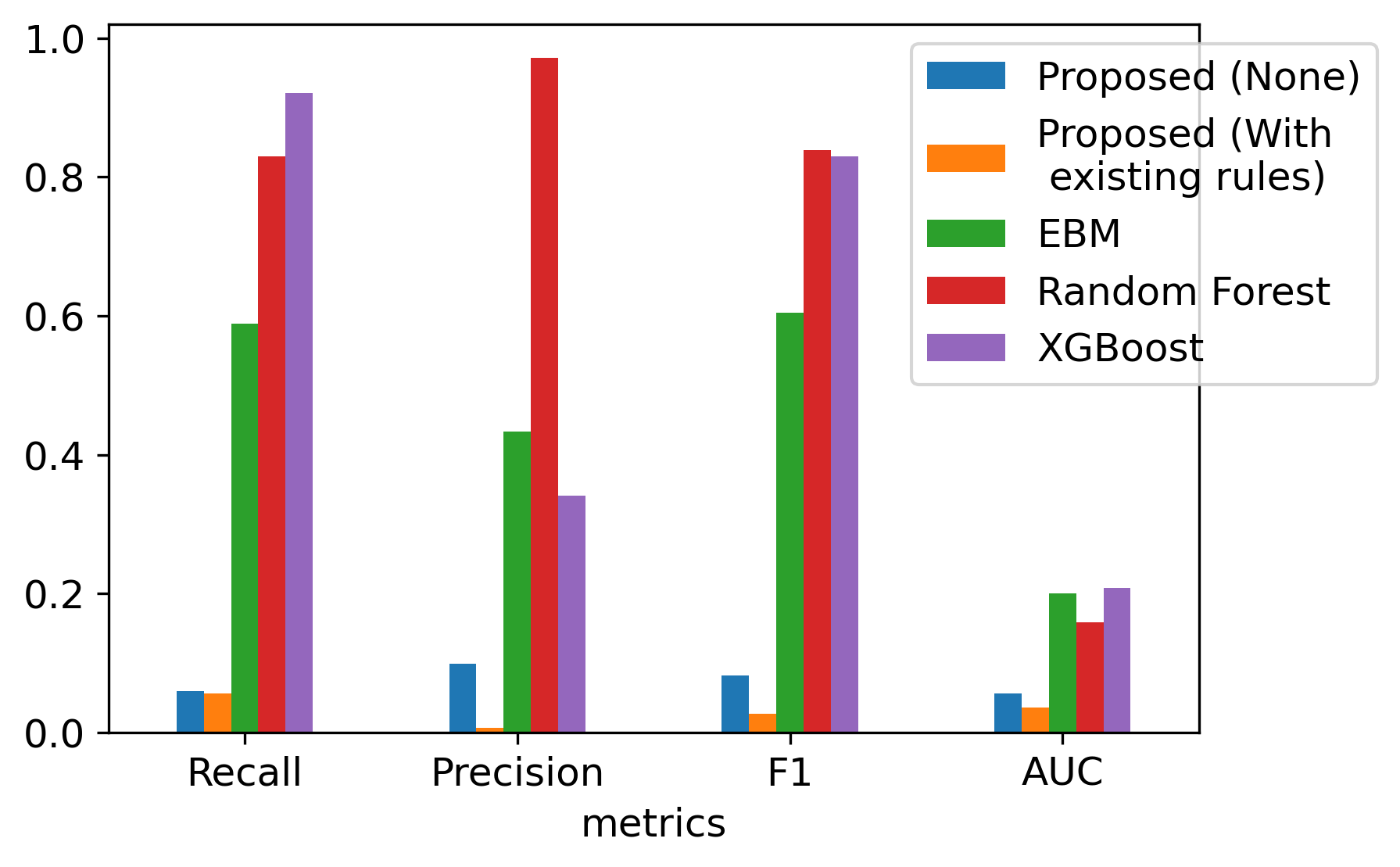
We applied the proposed network to identify patients that are eligible for advanced therapies. From Table VI, initializing the network with existing knowledge can greatly facilitate model performance. The proposed method had a lower AUC compared with EBM, Random Forest, and XGBoost. However, those models have low values in recall and F1-score, which means they tend to classify all samples as “negative”. In addition, those three methods achieved very high values on the validation set for all metrics, and this indicates severe overfitting on the validation set. Figure 5 shows the generalization error between validation set and test set for five ML models. We can find the generalization errors for EBM, Random Forest, and XGBoost are very high. In contrast, the proposed method had a significantly smaller generalization error. Notably, integrating existing domain knowledge can not only improve the classification performance, but also further reduce the generalization error.
Figure 6 shows the learned rules of the trained model initialized with existing knowledge. These learned rules approximated those provided by heart failure cardiologists though in unique combinations and with additional learned features. All of the rules from heart failure cardiologists included a reduced ejection fraction and an objective marker of significant functional limitations, most often by cardiopulmonary exercise testing. As seen in Figure 6, almost all rules learned by the model included ejection fraction as well as a second variable denoting a patient’s functional tolerance, either by cardiopulmonary exercise testing, 6-minute walk distance, or by gait speed. Notably, while gait speed is an objective and valid measure of functional capacity, it was not included in any of the provided rules and thus represents learned knowledge.
VI Conclusion
In this study, we proposed a novel machine learning model that is transparent and interpretable. The proposed network was tested on both synthetic datasets and a real-world dataset. Our experimental results show that (1) the model can learn hidden rules from the dataset and represent them in a way that humans can understand; (2) the introduction of the smoothness factor enables the model to find the most suitable encoding functions and aggregation operators, which increases the performance of the proposed method; and (3) initializing the network with existing approximate domain knowledge can effectively improve model performance and generalizability, especially when the size of the training set is limited. Notably, the proposed network shows significantly improved generalizability when identifying patients with heart failure who would benefit from advanced therapies. The proposed algorithm is promising in building multiple other clinical (and non-clinical) decision-making applications.
The proposed network will be further extended and explored in future work. In the current optimization method, we use the same smoothness factor for encoding membership functions and aggregation operators. A simple linear decrease with the training steps was performed to optimize the smoothness factor. In future work, we will explore the possibility of optimizing the smoothness factors individually in respective modules with a more effective optimization method.

ACKNOWLEDGMENT
The work was supported by the National Science Foundation under Grant No. 2014003.
References
- [1] K. S. Parikh, K. Sharma, M. Fiuzat, H. K. Surks, J. T. George, N. Honarpour, C. Depre, P. Desvigne-Nickens, R. Nkulikiyinka, G. D. Lewis et al., “Heart failure with preserved ejection fraction expert panel report: current controversies and implications for clinical trials,” JACC: Heart Failure, vol. 6, no. 8, pp. 619–632, 2018.
- [2] E. Benjamin, S. Virani, C. Callaway, A. Chamberlain, A. Chang, S. Cheng, S. Chiuve, M. Cushman, F. Delling, R. Deo et al., “American heart association council on e, prevention statistics c, stroke statistics s (2018) heart disease and stroke statistics-2018 update: a report from the american heart association,” Circulation, vol. 137, no. 12, pp. e67–e492.
- [3] N. Noorbakhsh-Sabet, R. Zand, Y. Zhang, and V. Abedi, “Artificial intelligence transforms the future of health care,” The American journal of medicine, vol. 132, no. 7, pp. 795–801, 2019.
- [4] S. Caccomo, “Fda permits marketing of artificial intelligence algorithm for aiding providers in detecting wrist fractures,” FDA News Release, 2018.
- [5] M. A. Myszczynska, P. N. Ojamies, A. M. Lacoste, D. Neil, A. Saffari, R. Mead, G. M. Hautbergue, J. D. Holbrook, and L. Ferraiuolo, “Applications of machine learning to diagnosis and treatment of neurodegenerative diseases,” Nature Reviews Neurology, vol. 16, no. 8, pp. 440–456, 2020.
- [6] J. T. Senders, P. C. Staples, A. V. Karhade, M. M. Zaki, W. B. Gormley, M. L. Broekman, T. R. Smith, and O. Arnaout, “Machine learning and neurosurgical outcome prediction: a systematic review,” World neurosurgery, vol. 109, pp. 476–486, 2018.
- [7] H. Yao, C. Williamson, J. Gryak, and K. Najarian, “Automated hematoma segmentation and outcome prediction for patients with traumatic brain injury,” Artificial Intelligence in Medicine, vol. 107, p. 101910, 2020.
- [8] T. Davenport and R. Kalakota, “The potential for artificial intelligence in healthcare,” Future healthcare journal, vol. 6, no. 2, p. 94, 2019.
- [9] L. A. Zadeh, “Fuzzy logic and approximate reasoning,” Synthese, vol. 30, no. 3, pp. 407–428, 1975.
- [10] T. Takagi and M. Sugeno, “Fuzzy identification of systems and its applications to modeling and control,” IEEE transactions on systems, man, and cybernetics, no. 1, pp. 116–132, 1985.
- [11] K. Y. Chan, S.-H. Ling, T. S. Dillon, and H. T. Nguyen, “Diagnosis of hypoglycemic episodes using a neural network based rule discovery system,” Expert Systems with Applications, vol. 38, no. 8, pp. 9799–9808, 2011.
- [12] R. Zhang and J. Tao, “A nonlinear fuzzy neural network modeling approach using an improved genetic algorithm,” IEEE Transactions on Industrial Electronics, vol. 65, no. 7, pp. 5882–5892, 2017.
- [13] G. Mikhalkin, “Tropical geometry and its applications,” arXiv preprint math/0601041, 2006.
- [14] F. Doshi-Velez and B. Kim, “Towards a rigorous science of interpretable machine learning,” arXiv preprint arXiv:1702.08608, 2017.
- [15] B. Mittelstadt, C. Russell, and S. Wachter, “Explaining explanations in ai,” in Proceedings of the conference on fairness, accountability, and transparency, 2019, pp. 279–288.
- [16] G. Louppe, “Understanding random forests: From theory to practice,” arXiv preprint arXiv:1407.7502, 2014.
- [17] F. Hohman, H. Park, C. Robinson, and D. H. P. Chau, “S ummit: Scaling deep learning interpretability by visualizing activation and attribution summarizations,” IEEE transactions on visualization and computer graphics, vol. 26, no. 1, pp. 1096–1106, 2019.
- [18] Y. Lou, R. Caruana, and J. Gehrke, “Intelligible models for classification and regression,” in Proceedings of the 18th ACM SIGKDD international conference on Knowledge discovery and data mining, 2012, pp. 150–158.
- [19] R. Caruana, Y. Lou, J. Gehrke, P. Koch, M. Sturm, and N. Elhadad, “Intelligible models for healthcare: Predicting pneumonia risk and hospital 30-day readmission,” in Proceedings of the 21th ACM SIGKDD international conference on knowledge discovery and data mining, 2015, pp. 1721–1730.
- [20] A. Stoica, “Synaptic and somatic operators for fuzzy neurons: which t-norms to choose?” in Proceedings of North American Fuzzy Information Processing. IEEE, 1996, pp. 55–58.
- [21] J.-S. Jang, “Anfis: adaptive-network-based fuzzy inference system,” IEEE transactions on systems, man, and cybernetics, vol. 23, no. 3, pp. 665–685, 1993.
- [22] A. F. Cabalar, A. Cevik, and C. Gokceoglu, “Some applications of adaptive neuro-fuzzy inference system (anfis) in geotechnical engineering,” Computers and Geotechnics, vol. 40, pp. 14–33, 2012.
- [23] M. Al-Mahasneh, M. Aljarrah, T. Rababah, and M. Alu’datt, “Application of hybrid neural fuzzy system (anfis) in food processing and technology,” Food engineering reviews, vol. 8, no. 3, pp. 351–366, 2016.
- [24] H. Yao, K. D. Aaronson, L. Lu, J. Gryak, K. Najarian, and J. R. Golbus, “Using a fuzzy neural network in clinical decision support for patients with advanced heart failure,” in 2019 IEEE International Conference on Bioinformatics and Biomedicine (BIBM). IEEE, 2019, pp. 995–999.
- [25] M. Sugeno and K. Tanaka, “Successive identification of a fuzzy model and its applications to prediction of a complex system,” Fuzzy sets and systems, vol. 42, no. 3, pp. 315–334, 1991.
- [26] C.-T. Sun, “Rule-base structure identification in an adaptive-network-based fuzzy inference system,” IEEE Transactions on Fuzzy Systems, vol. 2, no. 1, pp. 64–73, 1994.
- [27] M. Pratama, J. Lu, E. Lughofer, G. Zhang, and M. J. Er, “An incremental learning of concept drifts using evolving type-2 recurrent fuzzy neural networks,” IEEE Transactions on Fuzzy Systems, vol. 25, no. 5, pp. 1175–1192, 2016.
- [28] O. A. M. Ali, A. Y. Ali, and B. S. Sumait, “Comparison between the effects of different types of membership functions on fuzzy logic controller performance,” International Journal, vol. 76, pp. 76–83, 2015.
- [29] J. G. Monicka, N. G. Sekhar, and K. R. Kumar, “Performance evaluation of membership functions on fuzzy logic controlled ac voltage controller for speed control of induction motor drive,” International Journal of Computer Applications, vol. 13, no. 5, pp. 8–12, 2011.
- [30] A. Sadollah, Fuzzy Logic Based in Optimization Methods and Control Systems and Its Applications. BoD–Books on Demand, 2018.
- [31] H. Nori, S. Jenkins, P. Koch, and R. Caruana, “Interpretml: A unified framework for machine learning interpretability,” arXiv preprint arXiv:1909.09223, 2019.
- [32] S. K. Meher, “A new fuzzy supervised classification method based on aggregation operator,” in 2007 Third International IEEE Conference on Signal-Image Technologies and Internet-Based System. IEEE, 2007, pp. 876–882.
- [33] P. Virtanen, R. Gommers, T. E. Oliphant, M. Haberland, T. Reddy, D. Cournapeau, E. Burovski, P. Peterson, W. Weckesser, J. Bright, S. J. van der Walt, M. Brett, J. Wilson, K. J. Millman, N. Mayorov, A. R. J. Nelson, E. Jones, R. Kern, E. Larson, C. J. Carey, İ. Polat, Y. Feng, E. W. Moore, J. VanderPlas, D. Laxalde, J. Perktold, R. Cimrman, I. Henriksen, E. A. Quintero, C. R. Harris, A. M. Archibald, A. H. Ribeiro, F. Pedregosa, P. van Mulbregt, and SciPy 1.0 Contributors, “SciPy 1.0: Fundamental Algorithms for Scientific Computing in Python,” Nature Methods, vol. 17, pp. 261–272, 2020.
- [34] C.-C. Chang and C.-J. Lin, “Libsvm: a library for support vector machines,” ACM transactions on intelligent systems and technology (TIST), vol. 2, no. 3, pp. 1–27, 2011.
- [35] T. Chen and C. Guestrin, “Xgboost: A scalable tree boosting system,” in Proceedings of the 22nd acm sigkdd international conference on knowledge discovery and data mining, 2016, pp. 785–794.
Appendix A Implementation of the established ML algorithms
Public Python packages were used to build the established ML classifiers with default settings except for specified hyperparameters to be tuned on the validation set.
- 1.
Logistic Regression: We used the Logistic Regression Classifier from sklearn[33].
- 2.
Naïve Bayes: We used Naive Bayes from sklearn.
- 3.
Decision Tree: We used Decision Tree Classifier from sklearn. The maximal depth of the tree and the minimum number of samples required to split were tuned.
- 4.
Random Forest: We used Random Forest Classifier from sklearn. The number of trees, the maximal depth of the tree, and the minimum number of samples required to split were tuned.
- 5.
SVM: We used Support Vector Classifier from sklearn, whose implementation is based on libsvm [34]. The regularization parameter, the kernel type (linear function, radial basis function, sigmoid function, or polynomial function), and kernel coefficient were tuned.
- 6.
XGBoost: We used the tree-based XGBoost Classifier from xgboost [35]. The number of boosting rounds, learning rate, maximal tree depth for base learners were tuned.
- 7.
EBM: We used the Explainable Boosting Classifier from interpret. The learning rate and ways of feature interactions were tuned.
- 8.