Optimal shape of stellarators for magnetic confinement fusion
Abstract
We are interested in the design of stellarators, devices for the production of controlled nuclear fusion reactions alternative to tokamaks. The confinement of the plasma is entirely achieved by a helical magnetic field created by the complex arrangement of coils fed by high currents around a toroidal domain. Such coils describe a surface called “coil winding surface” (CWS). In this paper, we model the design of the CWS as a shape optimization problem, so that the cost functional reflects both optimal plasma confinement properties, through a least square discrepancy, and also manufacturability, thanks to geometrical terms involving the lateral surface or the curvature of the CWS.
We completely analyze the resulting problem: on the one hand, we establish the existence of an optimal shape, prove the shape differentiability of the criterion, and provide the expression of the differential in a workable form. On the other hand, we propose a numerical method and perform simulations of optimal stellarator shapes. We discuss the efficiency of our approach with respect to the literature in this area.
Keywords: shape optimization, plasma Physics, Biot and Savart operator, Riemannian manifolds.
AMS classification (MSC 2020): 49Q10, 49Q12, 78A25, 65T40.
1 Introduction
1.1 Motivations: towards a shape optimization problem
Nuclear fusion is a nuclear reaction involving the use of light nuclei. In order to produce energy by nuclear fusion, high temperature plasmas11 1 This is a particular state of matter when it becomes totally ionized, i.e., when all its atoms have lost one or more peripheral electrons. This is the most common state of matter in the universe because it is found (at 99%) in the stars, the interstellar medium, and earth’s ionosphere. must be produced and confined. For these reactions to occur, the nuclei must get close to each other at very small distances. They must therefore overcome the Coulomb repulsion. This happens naturally in a plasma during collisions if the energy of the nuclei is sufficient. This is the objective of devices called tokamaks, steel magnetic confinement chambers that allow a plasma to be controlled in order to study and experiment with energy production by nuclear fusion. The magnetic confinement technique allows to maintain a sufficient temperature and density of the plasma, in an intense magnetic field. The simplest configuration for the magnetic field is the toroidal solenoid; this is the configuration found in most current experiments.
Unfortunately, the magnetic field is not uniform in general, which causes a vertical drift of the particles, in opposite directions for the ions and for the electrons. This charge separation creates a vertical electric field which, in turn, causes the particles to drift out of the torus. This phenomenon dramatically reduces the confinement. To get around this obstacle, the effect of such drifts is canceled by giving a poloidal component22 2 The terms toroidal and poloidal refer to directions relative to a torus of reference. The poloidal direction follows a small circular ring around the surface, while the toroidal direction follows a large circular ring around the torus, encircling the central void. to the magnetic field: the field lines are wound on nested toroids. Thus, the particles, following the magnetic field lines, have their vertical drift cancelled at each turn. In a tokamak, the poloidal magnetic field is created by a toroidal electric current circulating in the plasma. This current is called plasma current.
A possible alternative to correct the problems of drift of magnetically confined plasma particles in a torus is to modify the toroidal shape of the device, by breaking the axisymmetry, yielding to the concept of stellarator. A stellarator is analogous to a tokamak except that it does not use a toroidal current flowing inside the plasma to confine it. The poloidal magnetic field is generated by external coils, or by a deformation of the coils responsible for the toroidal magnetic field. This system has the advantage of not requiring plasma current and therefore of being able to operate continuously; but it comes at the cost of more complex coils (non-planar coils) and of a more important neoclassical transport [15].
The confinement of the plasma is then entirely achieved by a helical magnetic field created by the complex arrangement of coils around the torus, supplied with strong currents and called poloidal coils.
Despite the promise of very stable steady-state fusion plasmas, stellarator technology also presents significant challenges related to the complex arrangement of magnetic field coils. These magnetic field coils are particularly expensive and especially difficult to design and fabricate due to the complexity of their spatial arrangement.
In this paper, we are interested in the search for the optimal shape of stellarators, i.e., the best coil arrangement (provided that it exists) to confine the plasma. In general, two steps are considered: first, the shape of the plasma boundary is determined in order to optimize the physical properties, among which the neoclassical transport and the magnetohydrodynamic (MHD) stability. In a second step, we search for the coil shapes producing approximately the “target" plasma shape resulting from the previous step.
In this article, we focus entirely on the second step, assuming that the target magnetic field is known. It is then convenient to define a coil winding surface (CWS) on which the coils will be located (see Figure 1). The optimal arrangement of stellarator coils corresponds then to the determination of a closed surface (the CWS) chosen to guarantee that the magnetic field created by the coils is as close as possible to the target magnetic field . Of course, it is necessary to consider feasibility and manufacturability constraints. We will propose and study several relevant choices of such constraints in what follows.

1.2 State of the art and main contributions of this article
The question of determining the best location of coils around a stellarator, reformulated as an optimal surface problem, is a major issue for the construction of stellarators with efficient confinement properties. The physical and mathematical literature dedicated to plasmas is rich of references on this issue. We mention hereafter a non-exhaustive list of various important contributions around this problem. Let us first mention [19], where all the basic theoretical elements to understand the modeling of stellarator magnetic fields are gathered.
Regarding optimal design issues, let us distinguish between several optimization/optimal control approaches and modeling choices. Each discrete stellarator coil can be represented as a closed one-dimensional curve embedded in [39, 40, 38]. In these references, several optimization methods are tested among which the steepest descent and Newton like methods.
Another common choice consists in using the aforementioned CWS, in other words to define a closed toroidal winding surface enclosing the plasma surface on which all coils lie. Two kinds of issues related to the optimal design of stellarators can then be addressed. The simplest is to assume the CWS to be given, and to look for currents on this surface generating the desired magnetic field for confining the plasma. Indeed, in the limit of a large number of coils, a set of discrete coils can be described by a continuous current density on the CWS. Let us mention NESCOIL [23, 29], where the current potential representing a surface current distribution is sought such that the normal component of the magnetic field vanishes in a least-squares sense at the plasma boundary. In the same vein, REGCOIL [21] improves the NESCOIL approach by adding a Tikhonov regularization term in the minimization functional whereas COILOPT [34] uses an explicit representation of modular coils on a toroidal winding surface. A review of such approaches can be found in [12]. Recently, a similar problem where an extra Laplace forces penalization term is taken into account has been investigated in [31].
A much more difficult problem is to determine the CWS and the density current distribution at the same time. This is expected to improve the performances of the resulting device. On the other hand, this approach requires solving a dual optimization problem, including a rather challenging surface optimization problem. This is the main purpose of this article. In the following we mention some of the many contributions on this topic and position our contribution through this literature. In [27], this problem is modeled using a cost functional written as the weighted sum of four terms: the first one is the surface-integrated-squared normal magnetic field on the desired plasma surface. The second is the opposite of the total volume enclosed by the coil-winding surface, acting to enforce the coil-plasma separation. The third one is a measure of the spectral width of the Fourier series describing the coil-winding surface. This allows to overcome the non-uniqueness of the Fourier series representation of the coil-winding surface. The last one is the norm of the current density, allowing to obtain coils with good manufacturing properties. It is important to note here, and this is related to the motivation for this paper, that the approach developed in [27] rests upon a (truncated) Fourier series parameterization of the surface equation. The authors thus compute derivatives of their cost with respect to these Fourier coefficients.
In [28], a more complex model involving a drift kinetic equation is considered and similar shape optimization issues are investigated.
In what follows, we propose a continuous approach, which does not rely on any parameterization of the surfaces involved. We use the notion of Hadamard variation and shape derivative. We rigorously analyze, in a continuous framework, the sensitivity with respect to the domain of a REGCOIL-type cost. We thus obtain intrinsic expressions with respect to any parametrization. This makes our approach flexible and the formulas obtained by using developments of the parametric equation of the surfaces in Fourier series can be adapted without any difficulty to other choices of parametrization. We also propose several choices of manufacturability terms in the cost functional and discuss their relevance.
The issues addressed in the following as well as our main contributions are summed-up hereafter:
- •
Modeling of the problem (Section 1.4). Using the CWS concept, we propose a continuous formulation of the question of the best coil arrangement as a shape optimization problem, regardless of any surface parametrization. In particular, several choices of manufacturing constraints are proposed. They are integrated to the cost functional using a penalization/regularization term. From the mathematical point of view, the main issue comes to minimize a functional involving the trace of the solution of an elliptic partial differential equation (PDE) on a manifold, under geometrical constraints involving the distance to this manifold.
- •
Analysis of the shape optimization problem (Sections 2 and 3). Having in mind the determination of an efficient algorithm for finding an optimal form for the above problem, we focus mainly on two questions. The first one is dedicated to the existence of an optimal shape (Section 2.2). In this context, the developed approach is not completely standard and requires to carefully establish semicontinuity properties of the trace of the solution of the PDE on manifolds satisying a uniform regularity property. The second one concerns the establishment of optimality conditions using the notion of form derivative (Section 3.2). Here again, due to the particular nature of the PDE at stake, the classical approach cannot be used in a direct way and many adaptations are necessary. We establish a workable expression of this derivative, which is the basis of the numerical approaches developed in the next section.
- •
Numerical implementation (Section 4). A relevant aspect of this paper is that the study of the sensitivity of the studied criterion to a variation of the shape of the stellarator is carried out without using any parameterization of the surface to be designed. As a result, the sensitivity relations obtained at the end of the previous step are totally intrinsic with respect to any parameterization of the surface. As a consequence, we can apply the more robust “optimize then discretize" approach, instead of a “discretize then optimize" procedure as in most of the methods implemented for this application. The shape derivatives constitute the basis of a quasi-Newton optimization method that we implement by using a parametric representation of the surface in terms of Fourier series.
1.3 Notations
In what follows, the notation is used to denote a toroidal surface33 3 By toroidal surface, we mean here the range of the toroidal solenoid by a homeomorphism. In what follows, we will rather consider smooth toroidal surfaces, where the wording “smooth” refers to at least regularity. in , equipped with the Riemannian metric induced by the canonical embedding , i.e., the scalar product between two vectors and tangent to at a common point is equal to , where denotes the Euclidean scalar product in . We also denote by the associated Riemannian volume form, which coincides with the two-dimensional Hausdorff measure on ([11, Theorem 2.10.10] and [10, Theorem 2 in Section 2.2]). We write to denote the bounded domain of such that .
Throughout this article, we use the following notation:
- •
For and any integer , denotes the -dimensional Hausdorff measure in ;
- •
denotes a smooth toroidal domain44 4 toroidal domain stands for any three-dimensional domain whose boundary is a toroidal surface of standing for the plasma domain;
- •
denotes the set of smooth tangent vector fields on ;
- •
denotes the completion of for the inner product
- •
denotes the cross product in ;
- •
given a function and , denotes the Jacobian matrix of . In the case where , stands for the absolute value of the determinant of . The symbol is used to denote the Jacobian operator with respect to the (vector) variable ;
- •
denotes the tangential gradient to in , defined for every differentiable function by on , where stands for the outward normal vector to . Similarly, the notation stands for the tangential divergence given by on , where is a vector field on ;
- •
The norm on induced by the inner product is denoted ;
- •
is the closure under the norm of the (tangential) divergence-free vectors of ;
- •
The flat two-dimensional torus is denoted by . , and are defined similarly to what has been done above;
- •
The Hausdorff distance and the signed distance from are defined as:
- •
If , the -tubular neighborhood of is the level set
of ;
- •
- •
Given a differentiable vector field , we denote by the symmetric part of the Jacobian matrix , that is,
(1) - •
For two Banach spaces and , we denote by the Banach space of continuous linear maps from to and by the Banach space of continuous endomorphisms;
- •
the adjoint of a linear operator is denoted by ;
- •
If and denote two matrices in , we define their doubly contracted product as
- •
denotes the identity matrix in .
1.4 Modeling: towards a shape optimization problem
Since we are interested in solving a shape optimization problem whose unknown is the coil winding surface , we are led to make some assumptions on motivated by the application under consideration. In particular, we assume in what follows that the distance between and the plasma domain is uniformly bounded from below, namely, we fix and we require that
| () |
We now introduce the main operator we will deal with, which plays a crucial role in electromagnetism: the so-called Biot and Savart operator. This operator associates with each current distribution on the corresponding magnetic field in . It can be considered as a kind of inverse of the curl operator.
Definition 1 (The Biot and Savart operator [9]).
Let be a smooth two-dimensional manifold and belong to . Let denote the single layer distribution supported on defined by
Let denote the unique distributional solution of the PDE
that falls off at infinity, i.e.,
Then the Biot and Savart operator is defined as the map associating with the restriction of to the plasma domain . By introducing the kernel given by
one has
| (2) |
Remark 1.
According to ( H dist , P , δ ), the restriction of to is uniformly bounded. By standard regularity results for parameterized integrals, the mapping is smooth and the operator , seen as going from to with , is continuous. As a consequence, the operator is compact.
In what follows, we will use several times that for every with we have
| (3) |
Computation of the optimal current .
In view of modeling the optimal design problem we will deal with, let us now introduce a target magnetic field .
The target magnetic field being given, we model the optimal design of a stellarator problem as a kind of regularized least square problem, where one aims at determining both the current and the manifold shape leading to the magnetic field closest to on . To this aim, and according to the REGCOIL procedure [21], we introduce the shape functional defined, for every closed smooth two-dimensional manifold , as
| () |
where denotes a regularization parameter.
The shape optimization problem.
To state the shape optimization problem that we will consider, let us first define the set of admissible manifolds. We gather hereafter several conditions evoked previously that we will take into account in the search of the CWS.
- •
Topology and uniform boundedness. To preserve the topology of the device (see Footnote 3), we will only consider CWSs that are two-dimensional closed toroidal manifolds. Moreover, we will fix a compact set of and we require the CWS to be contained in .
- •
Uniform distance constraint of the coils to the plasma. To build the vacuum vessel around the plasma, we will assume that the CWS satisfies assumption ( H dist , P , δ ).
- •
Manufacturing cost. In order to avoid irregular shapes that are too difficult to build, we will assume that the CWS has a minimal regularity, say , and a minimal reach condition. More precisely, we will assume that the reach of the CWS is uniformly bounded from below by some . We recall that this condition imposes that the curvature radii (where they can be defined) are larger than and that there is no bottleneck of distance smaller than (see, e.g., [1, Figure 3]). To sum-up,
() As it will be emphasized in what follows, the regularity assumption is actually a consequence of the reach constraint: indeed, the class of sets satisfying a “Reach” constraint is closed in a sense to be specified later and all elements are of class .
Other constraints such as a bound on the two-dimensional Hausdorff measure of (in other words the perimeter of the stellarator in ) will also be considered:
()
To sum-up, let us introduce the admissible set of shapes we will deal with in what follows:
Note that the reach condition has been imposed on the surface and not only on the volume.
The resulting shape optimization problem we will consider reads
| () |
In the two following sections, we investigate two important aspects of the shape optimization problem ( P shape ). The first one concerns the existence of optimal shapes and is investigated in Section 2. The second one is related to the derivation of first order optimality conditions, at the heart of the algorithms implemented in the last section of this article. To this aim, we apply in Section 3.2 the so-called Hadamard boundary variation method recalled in Section 3.1.
2 Existence issues for Problem ( P shape )
2.1 Existence of an optimal current for a given shape (Solving of Problem ( P S ))
We first establish that the infimum defining ( P S ) is in fact a minimum. Moreover, the minimizer is unique.
Lemma 1.
Let . The optimization problem ( P S ) has a unique minimizer . Moreover, one has
| (4) |
Proof.
First observe that is a Hilbert space and that the mapping is strongly convex, since it is the sum of the convex functional and the strongly convex one . Furthermore, we claim that the functional is lower semicontinuous for the strong topology of . Indeed, let denote a sequence of converging to . According to ( H dist , P , δ ), by using the dominated convergence theorem and since is uniformly bounded in , one has
It follows that the functional to minimize is lower semicontinuous (and even continuous) in , whence the existence of a unique minimizer for Problem ( P S ).
Since is continuous, its adjoint is well defined on . It is hence standard that the first order optimality condition for this problem reads
| (5) |
which also rewrites
Since is arbitrary in , we thus infer that . The operator is compact and symmetric. Besides its spectrum is positive and we can therefore consider its resolvent for negative real numbers with , so that
The expression of given in (4) follows from a straightforward computation. ∎
Remark 2.
When confronted with the numerical implementation of the shape optimization, motivated by the structure of and the properties of the in vacuo Maxwell-equations, we will find it useful to:
- •
optimize on a closed affine subset instead of the entire set . We refer to Section 4.1.3 for further details;
- •
replace the target magnetic field in by its normal component on the plasma surface (thus, by an object in ). Indeed, a divergence-free vector field on a 3D domain (in absence of electric currents in the plasma) is nearly entirely characterized by its normal component on the boundary. Further details are given in Section 4.1.2 and Appendix A.3.
Nevertheless, such changes have a minor impact on the theoretical discussion on the shape optimization process and we believe that, for the sake of clarity, it is better to postpone the details about such modifications to Section 4.
2.2 Existence of an optimal shape
Theorem 1.
The shape optimization problem ( P shape ) has at least one solution.
The proof follows the direct method of the calculus of variation. Most of the compactness on our set of admissible shapes comes from the bounded reach assumption ( H reach , r min ). In particular, the following Lipschitz estimate is crucial.
Lemma 2 (Theorem 2.8 of [4]).
Let be a nonempty set such that and . Then, for every , the gradient of the signed distance function is -Lipschitz on the tubular neighborhood .
With this estimate, we can state the following compactness result.
Lemma 3.
Let be in and denote by a sequence in . Then, there exists such that, up to a subsequence,
- •
is in and converges to in ;
- •
converges to in ;
- •
converges to in ;
- •
converges to .
Proof.
Compactness properties among Hausdorff distances from sets of uniformly positive reach are well known and remain valid for the signed distance (see, e.g., [7, Chapter 6]). Besides, as stated in [4], the convergence property holds true for the strong topology of (for ) and for the weak topology of in a tubular neighborhood of . As a consequence, and . In particular, thanks to Lemma 2, is on . Finally, the convergence of to follows from standard results on the continuity of (see [4] or [13]). ∎
The end of this section is devoted to the proof of Theorem 1. Let be a minimizing sequence for Problem ( P shape ). Denote by a closure point of this sequence in the sense of Lemma 3. In what follows, we will still denote by the converging subsequence introduced in Lemma 3.
We will proceed by showing a semicontinuity property of the criterion, namely that
Let denote the minimizer of Problem ( P S ) for the surface , whose existence is provided by Lemma 1.
The idea is to consider a volume integral as approximation of the surface integral in the same spirit as in [6]. For this purpose, we need to extend locally to a volume around . Notice that, without loss of generality, is contained in for every , which implies, in particular, that is everywhere defined and Lipschitz continuous on . Let be a small constant to be fixed later and define the map
where denote the image of . Notice that is a bijection between and if the latter is contained in (see Figure 2).
The differential of at reads
where is a matrix, according to the notation introduced in Section 1.3, and is identified with a linear subspace of . We can identify with a matrix by choosing an orthogonal basis on and its determinant, denoted in what follows, is independent of such a choice.


Using the regularity of near the surface , one can prove the following crucial estimate.
Lemma 4.
For every , there exists such that
for every large enough.
Proof.
By Lemma 3, is in a neighborhood of , thus is Lipschitz continuous for large enough with a Lipschitz constant independent of and, in particular, there exists such that for all large enough
Besides, the linear mapping is direct and orthogonal since is the unit normal outward vector. Hence, its determinant is equal to 1. Since the determinant is , we have
where the reminder term is uniformly bounded with respect to for large enough. This concludes the proof. ∎
In what follows is a small parameter to be fixed and is as in the statement of Lemma 4. We shall also assume that for every . Notice that, as soon as , for large enough is a diffeomorphism. Thus we can define on the projector onto along the field by requiring that coincides with the -component of the inverse of (see Figure 3).
This allows us to introduce , defined on by
Using [7, Chap. 7, theorem 8.5], for any large enough, we get
| (6) |
on . Moreover, converges uniformly to in a neighborhood of , since for every one has
where the limit is a consequence of Lemma 3.
Using the change of variable formula (also known as area formula for Lipschitz functions), one gets for large enough, every , and every ,
which also rewrites
| (7) |
Let be in and be small enough so that and , that is . Since in , there exists such that for all ,
| (8) |
Using that with Equation (6), we obtain
| (9) |
which ensure that belongs to . (Notice however that is not necessarily in , as it is neither, in general, a tangent vector field nor a divergence free one.) Equation (9) actually shows that is bounded in . Up to subsequence, it converges weakly to with
The remaining two steps of the proof consist first in showing the semicontinuity property
| (10) |
and then in checking that belongs to . Notice that, even if we have defined the operator only among the vector fields tangent to , by a slight abuse of notation it still makes sense to consider , defined using formula (2), even without having checked that is in .
Both steps rely on the following lemma.
Lemma 5.
Given and , there exists such that for every and every such that and is -Lipschitz continuous on , we have
for .
Proof.
Let and be such that and is -Lipschitz continuous on . Up to taking small enough, we can assume that
| (11) |
As above, consider , , and large enough so that (8) holds true. By (7), we have
where, for notational simplicity, we write for and for . Hence,
where we added and subtracted to get
We are going to show that and can be made arbitrarily small by suitably choosing and (depending only on and not on the specific function ) and letting be large enough.
The term can be estimated using the inequality , as follows:
where the factor comes from the fact that the measure of is equal to . Notice that is bounded uniformly with respect to , so that can be made arbitrarily small by choosing small enough (depending only on ).
Hence, we have the estimates
Hence can be made arbitrarily small choosing and then small enough, and letting large enough. ∎
Let us start the proof of (10) by comparing and . Given , one has
Notice that is bounded in a neighborhood of , uniformly with respect to , since . Moreover, for every and every , the map is upper bounded by outside according to (3). Assume that , so that is at distance at least from for every . Consider and a Lipschitz neighborhood of not intersecting . Since the geodesic distance in is equivalent to the restriction to of the standard Euclidean distance, we deduce that there exists independent of such that
We deduce from Lemma 5 that for every there exists such that for any integer ,
and, in particular,
Using the compactness of , we have
This concludes the proof of (10), since is arbitrary.
To conclude the proof, it remains to check that belongs to . By weak convergence of to and according to Lemma 5,
where we used that is orthogonal to everywhere on . According to Lemma 2, moreover,
and we conclude that since the sequence is bounded. This proves that is a vector field tangent to .
To prove that is divergence free (in distributional sense), we have to check that is orthogonal to . Indeed, this characterization of divergence-free vector fields follows from the Hodge decomposition (see Appendix A.1). For , since on , one has
Set for . Notice that converges uniformly to in a neighborhood of . Hence, again using Lemma 5,
This concludes the proof of Theorem 1.
3 Shape differentiation for Problem ( P shape )
3.1 Reminders on the Hadamard boundary variation method
Let us recall hereafter some notions of topology on sets of regular domains defined in terms of particular perturbations called identity perturbations. The latter are of the form , where is small enough in a suitable sense. More precisely, according to the approach developed in [26, 25], one defines
and
with .
Let us recall that the space endowed with the norm
is a Banach space. Choosing in allows to preserve the topological and regularity properties of sets we are interested in, as highlighted in the next result.
Lemma 6.
Let be an open bounded subset of and let .
- •
If is of class , then is an open bounded domain whose boundary is of class . Furthermore, one has .
- •
If is such that , then .
The first statement of this lemma follows from standard arguments. For instance, the property “” directly results from the fact that defines a homeomorphism. The second one comes from a direct application of the Banach fixed-point theorem. We refer to [7, Chapter 4] for more explanations.
As a consequence of the lemma, induces a topology on the set of open sets of whose boundary belongs to (according for instance to [26, Assertion 2.52]). Given , let be the set of domains of the type with and small enough so that is a diffeomorphism (Lemma 6). Then, one defines a topology on the space with the help of the neighborhood basis given by the sets of . Furthermore, it is shown in [24] that every neighborhood of in is metrizable with a Courant-type distance (induced by that associated with in ) and has the structure of complete separable manifold.
Let us conclude this section by recalling the notion of shape differentiability.
Definition 2.
A shape functional is said to be shape differentiable at (in the sense of Hadamard) in the class of domains with boundary whenever the underlying mapping
with , is differentiable in the sense of Fréchet at . The corresponding differential is the so-called shape derivative of at and, by definition of Fréchet differential, the following expansion holds:
In the next section we study the shape differentiability of the cost . In order to fit Definition 2, is implicitly identified with a functional on the set of toroidal domains.
3.2 Shape derivative of the cost functional
This section and the next one are devoted to the computation of the shape derivative of the functional .
Theorem 2.
Let . Let and , a bilinear mapping from into , defined by
The functional defined by ( P S ) is shape differentiable at . Moreover, for every one has
with
where for , denotes the -th line of seen as a column vector, and denotes the outward normal vector to .
Remark 3.
The proof of this result relies crucially on the expression of the magnetic field provided through the Biot and Savart operator (see Definition 1). In general, in many shape optimization problems involving PDEs on bounded domains, PDEs are interpreted as implicit equations on the deformation variable and on the state variable. They are in general taken into account by applying the implicit function theorem which also provides an expression for the material (or Lagrangian) derivative of the state with respect to the deformation (see, e.g., [16, Chapter 5]). In the present case, dealing with the Biot and Savart operator comes to consider a PDE on an unbounded domain. The approach we have chosen here, instead, is based on the integral representation of the state variable (the magnetic field here). To establish the above result, we use suitable changes of variables that allows us to rewrite the criterion as an integral over a fixed domain and derive it as a parameterized integral with respect to . Although the principle of this calculation is simple, its implementation is not straightforward.
3.3 Proof of Theorem 2
For the sake of notational simplicity, the inverse of a group element will be denoted with a slight abuse of notation by .
Let and be as in the statement of the theorem. Assume for now that the criterion is shape differentiable at . We will comment on this assumption at the end of the proof. In what follows, we concentrate on the computation of the shape derivative in the direction .
Since is shape differentiable at , we infer that
Step 1: a change of variable.
In order to compute , we need to compute some kind of derivative of and its adjoint. Nevertheless, we aim to overcome the fact that the domain of depends on .
Notice that, according to the discussion in Section 3.1, the mapping induces a bijection between and . Nevertheless does not map into . This leads us to introduce the linear mapping
| (12) |
where denotes the Jacobian determinant55 5 Note that is not the determinant of the three-dimensional mapping but the determinant of the restriction of this application from (the tangent space of at ) into . of (see Appendix C for further details and the explicit expression of ).
The following result will be crucial in what follows since it confirms that is indeed a diffeomorphism preserving divergence-free vector fields.
Lemma 7.
For every small enough, is a diffeomorphism from to .
Proof.
Since is an orientation preserving diffeomorphism, one has . Besides,
As a consequence, defines a diffeomorphism from to . We are left to prove that it preserves divergence-free vector fields. According to the Hodge decomposition (see Appendix A.1), it is enough to check that is orthogonal to . Using the change of variables formula (cf. (28)), one has, for every ,
where the notation stands for the conormal derivative of . Then is divergence-free if and only if is. The lemma is thus proved. ∎
Step 2: computation of the variation of .
Since we prefer to avoid dealing with operators defined on , we will use to relate and .
Let us first compute . Let and . One has
We thus infer that is given by
Let . According to Lemmas 1 and 7, is well defined and belongs to . To compute the differential of , it is convenient to introduce the operators
so that
According to the optimality condition (5) on , is uniquely characterized by the identity
which also rewrites
It follows that
| (13) |
Let us now compute the first order variation of . To this aim, we use the expansion
| (14) |
obtained in [16, Lemma 5.4.15]. Recall that the notation stands for the tangential divergence of on .
Lemma 8.
Proof of Lemma 8.
Let us start with . Given and , we have
| (16) |
Moreover, it can be easily checked that the reminder term of this expansion grows at most linearly with respect to . Regarding , a similar reasoning using (14) yields
concluding the proof. ∎
Combining all the results above, we now compute the sensitivity of with respect to . The following result is an immediate consequence of Lemma 8 and (13).
Proposition 1.
One has with
Step 3: computation of the cost functional derivative.
Recall that
| (17) | |||||
By differentiating this expression and according to Proposition 1, we get
Note that
Thus
| (18) |
Remark 4.
The previous expression can be understood as follows: writing with the natural choice of and assuming that and are sufficiently regular, one has
Using the fact that since is the minimizer of , we get
In what follows, we will use the identity stated in the following lemma.
Lemma 9.
Let , , and be as in the statement of Theorem 2. Then
Proof.
The proof follows from straightforward computations, by combining the Fubini theorem with standard properties of the scalar triple product66 6 Recall that the scalar triple product of three vectors is given by and coincides with the (signed) volume of the parallelepiped defined by the three vectors. Therefore, the scalar triple product is preserved by a circular shift of the triple .. ∎
To conclude this computation, observe that for all vectors and in ,
so that
We thus obtain
where and have been introduced in the statement of the theorem.
Now, according to [16, Prop. 5.4.9], the shape differential above can be recast as
where, for , denotes the -th line of seen as a column vector, is the tangential part of defined as , and denotes the mean curvature77 7 The mean curvature of a surface is defined here as the sum of the principal curvatures of . on . The expected formula is obtained by noting that each line of is tangential (in other words, normal to ). Indeed, this follows from the definitions of the mapping , the function , and the fact that corresponds to the matrix of the orthogonal projection onto .
To conclude this proof, it remains to investigate the shape differentiability of . Let us introduce where is chosen as in the statement of the theorem. It is straightforward to show that the real number can be written as a smooth function of integrals written on the fixed domain , for which the integrand depends regularly on . Indeed, this can be straightforwardly obtained by replacing by in the reasoning above, and mimicking the associated computations leading to (13), (16) and (17). This yields to the expansion
with and the shape differentiability of hence follows.
4 Numerical implementation
The results obtained above are intrinsic in the sense that they do not depend on the parametrization of the objects (surfaces, magnetic field, electric current, …). There are several ways to represent them numerically. We have chosen to use what is, to the best of the authors’ knowledge, the classical approach in the stellarator community. In particular:
- •
Surfaces, vector fields and magnetic fields are represented by Fourier coefficients. We detail the parametrization in Section 4.1.
- •
- •
As mentioned in Remark 2, is slightly modified. Not only the optimization space is replaced by a suitable affine subspace of it, but also we restrict the image of to the plasma boundary. We provide further details in Sections 4.1.3 and 4.1.2 and Section A.3.
4.1 Parametrization issues
4.1.1 Surface representation
We represent a toroidal surfaces as the image of the two-dimensional flat torus by an embedding
Stellarators often exhibits a discrete symmetry by rotation. For example W7X is invariant by the rotation of angle along the vertical axis and NCSX has an invariance by the rotation of angle . To reduce the complexity, we only represent one module of the surface and we denote by the number of modules needed to generate the entire surface (using rotations of angle ). We introduce the cylindrical coordinates . We will make the assumption of no toroidal folding, i.e., that the intersection of each half plane with is a single loop. We express in cylindrical coordinates as
Then we develop and in Fourier components and we impose the stellarator-symmetry
| (19) | ||||
| (20) |
Note the absence of terms for and terms for . For the numerical simulation, we truncate the number of Fourier components in (19) and (20).
Remark 5.
The cost considered in this paper only depends on the surface (and is independent of its parametrization ). On the toroidal direction, we have already imposed that . On the other hand, we can compose with any diffeomorphism on the poloidal direction . Namely, and have the same image for a fixed . Thus our problem is invariant under the action of a smooth family of diffeomorphisms. This extra degree of freedom has two consequences:
- •
If we use a regular discretization for the surface of size , we need and to be as regular as possible.
- •
As we take a finite number of harmonics, we would like to “compress" as much as possible the information on the shape by using low harmonics.
This problem has been study in the plasma community in [17] and gave rise to the notion of spectrally optimized Fourier series. Nevertheless, we would like to highlight that this approach is extrinsic (it depends on the parametrization) and should not be used for other purposes than fixing the gauge invariance. We have not implemented it since our numerical results empirically already provided a reasonable regularity on the poloidal parametrization.
4.1.2 Magnetic field representation
In the previous sections, we represented the target magnetic field as a three-dimensional vector field in the plasma domain. Nonetheless, thanks to the structure of Maxwell’s equations, the magnetic field inside is nearly entirely determined by its normal component along . It is thus possible to work with a scalar quantity on a surface instead of a three-dimensional vector field on a volume. Indeed, let us introduce the line integral (also called circulation) of the magnetic field along one toroidal turn. By Stoke’s theorem (also known as Ampere circuital law in electromagnetism), this is equal to the total flux of the electric current across any surface enclosed by the above-mentioned toroidal loop. This quantity is called the total poloidal current and is denoted by .
As proved in Appendix A.3, and the normal component of the magnetic field across characterize completely the magnetic field inside the plasma.
As a consequence, it is reasonable to minimize
with the total poloidal current of fixed, where denotes the outward normal unit vector to .
This idea has been used by physicists for a long time, for example [23, 21]. Besides, if we consider two currents distribution and on two toroidal surfaces and outside of with the same total poloidal currents, the induced magnetic field in satisfies
We provide mathematical proofs of these facts in Appendix A.3.
We also use a normal target magnetic field that respects the stellarator symmetry, that is,
As before, we truncate the Fourier series to obtain a numerically tractable expression.
4.1.3 Current-sheet representation
As mentioned in the previous section, we need to parameterized all divergence-free vector field on with a fixed total poloidal current . In Appendix A.2 we prove that
| (21) |
with .
The following lemma describes how embeddings induce isomorphisms between and .
Lemma 10.
Let be an embedding with and consider
Then induces an isomorphism between and .
The proof is completely similar to that of Lemma 7.
Let us suppose now that are poloidal and toroidal coordinates for the parameterization , that is,
- •
is a loop doing exactly one poloidal turn (and 0 toroidal ones);
- •
is a loop doing exactly one toroidal turn (and 0 poloidal ones).
Besides, as is it in general the convention in the dedicated literature, we assume that is orientation reversing, meaning that
| (22) |
with the outward normal vector field.
Lemma 11.
Let . Then the poloidal (respectively, toroidal) flux of , i.e., the flux of across (respectively, ), is given by (respectively, ).
Proof.
Remark that ensure that the flux across any loop depends only on the isotopic class of the loop considered. Recall that the flux of across some loop is given by
where the choice of the sign in is due to to the convention (22). Thus, the flux across (the poloidal flux) is
The computation of the flux across is analogous. ∎
Thanks to this lemma, in order to minimize on we fix and and minimize with respect to . Indeed, is fixed by the toroidal circulation of the target magnetic field (see A.3), whereas is usually set to 0. This second condition is necessary to ensure the existence of “poloidal coils". Otherwise, no closed field lines would realize one poloidal turn and zero toroidal ones. Thus, the set of admissible currents is described by
We say that is the scalar current potential. By stellarator symmetry, its expansion in Fourier series is
Let us denote
It is straightforward that the affine decomposition is compatible with (cf. (12)), meaning that for any shape deformation ,
Thus, we can consider the restriction of to that we will denote . Let be its adjoint (in ) and the orthogonal projector defined in onto . Then Lemma 1 holds and the expression of the unique minimizer is given by
4.2 Implementation
We wrote our implementation in python using several scientific computing open source libraries and, in particular:
- •
Numpy [14] for array computation,
- •
Scipy [36] for the implementation of the Broyden-Fletcher-Goldfarb-Shanno (BFGS) minimization algorithm,
- •
Opt_einsum [32] for optimizing tensor construction,
- •
Dask [5] for large array and efficient scientific computing parallelization,
- •
The full code is available on our gitlab88 8 https://plmlab.math.cnrs.fr/rrobin/stellacode under MPL 2 license.
The constraints on the perimeter, the reach and the plasma-CWS distance are implemented as a nonlinear penalization cost which blows up rapidly once the values exceed (or subceed) a given threshold. We refer to the code documentation for further details99 9 https://rrobin.pages.math.cnrs.fr/stellacode/.
4.3 Numerical results
In what follows, the data used for the simulations come from the NCSX stellarator equilibrium known as LI383 [37]. We will also use as reference CWS the one used in the original REGCOIL paper [21].
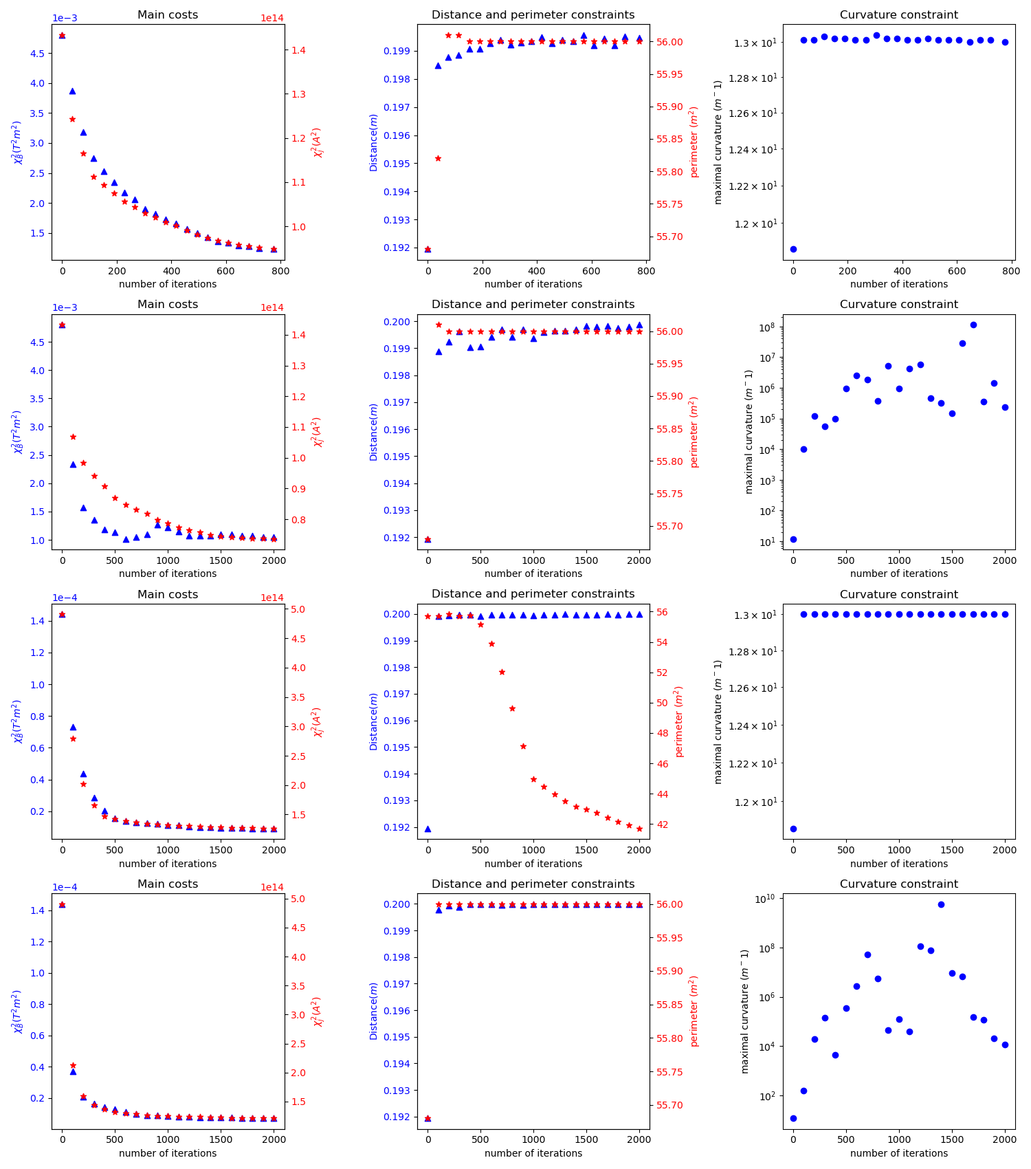
We present here four simulations. We used either or as regularization parameter in the expression of the cost . We mesh the CWS and the plasma surface with grids. The scalar current potential is developed in Fourier series up to order 12 in both directions. The optimization is performed with up to steps of the BFGS algorithm. In every simulation we implemented a penalization on the perimeter of the CWS (penalization above m2) and on plasma-CWS distance (penalization under cm). We also implemented a reach penalization for two simulations (penalization under cm). Let us call Ref the initial CWS. We use DP to refer to the simulations with distance and perimeter penalization and DPR for those with additional reach penalization. The numerical results are summarized in Tables 1 and 2. Figure 7 illustrates the convergence history of the implemented optimization algorithm.
Remark 6.
Without penalization on the reach, one naturally obtains better results (as less constraints are applied on the set of admissible shapes). Nevertheless, such an approach seems a very bad idea:
- •
theoretically, since the existence of an optimal shape is guaranteed only for bounded reach,
- •
numerically, because sharper and sharper “spikes" appear, as shown in Figure 6. Those spikes can be arbitrary long while still keeping a finite perimeter (and encapsulated volume).


Appendix A Some differential geometry
In this section, we recall some basics fact about differential geometry and vector fields on toroidal surfaces and domains.
A.1 Hodge decomposition
We recall in this part some notions of differential geometry and in particular of Hodge theory. We refer to [20, Chapter 3] and [22] for details and precise definitions in the smooth setting. Although we are only interested in manifolds in this article, note for the sake of completeness that details on Hodge theory for Lipschitz manifolds can be found for instance in [35].
The Hodge decomposition is a powerful tool which gives an orthogonal decomposition of the space of square integrable -forms on a Riemannian closed manifold as
where is the -closure of , is the -closure of ( is the coderivative), and is the set of harmonic -forms with the Hodge Laplacian.
We apply this result to the simple case of 1-forms on a two-dimensional closed Riemannian manifold . We recall a few basics facts:
- •
1-forms and vector fields can be identified thanks to the Riemannian metric. This isomorphism is called the musical isomorphism and we denote by the 1-form defined as the image of a vector field thought the musical isomorphism. Conversely denotes the vector field which is the image of the 1-form .
- •
The divergence of a vector field is .
- •
and .
- •
is equivalent to the system of equations
We want to show that the space of “divergence-free" 1-forms (i.e., ) coincides with . It is clear that the latter space is contained in . Conversely, for every exact form , i.e., such that with , one has . We recall that the Hodge Laplacian coincides with the Laplace–Beltrami operator on 0-forms. But implies that is constant on each connected component, thus implies that . As a result the space of divergence-free 1-forms is .
Equivalently, the space of divergence-free vector fields coincides with the orthogonal to . In Appendix A.2 we give an explicit description of for the two-dimensional flat torus.
A.2 Divergence-free vector field on a flat torus
Let be the flat torus with Cartesian parametrization . We want to characterize the set of divergence-free vector fields on .
As explained in A.1, we only need to characterizes and .
- •
is the -closure of the 1-forms for .
- •
is a two-dimensional vector space as the first Betti number for a 2D torus satisfies . We easily compute .
Using the musical isomorphism, we deduce that all divergence-free vector fields in have the form given in Equation (21).
A.3 Poisson equation on a toroidal 3D domain
Given a toroidal 3D domain , we want to study the Maxwell equations in vacuum inside . We introduce a toroidal loop inside and denote by the electric current-flux across any surface enclosed by . By the conservation of charges (), this quantity is well defined. By smoothness of the Biot and Savart operator and of the plasma boundary , all functions considered in this appendix may be assumed to be .
Lemma 12.
Let be the normal magnetic field on (i.e., the normal component of ). Then and determine completely the magnetic field in . Besides, there exists a constant such that for every other magnetic field with the same total poloidal current, where is the normal component of .
Before going to the proof of this statement, we emphasize that the structure of the space is well understood and admits a generalized Hodge decomposition ( is not a closed manifold, thus part A.1 does not apply) from which the lemma follows easily. Such a decomposition is proved, for example, in [3]. For completeness, we provide the following proof.
Proof.
We have the cochain complex (meaning and )
For simply connected domains of , the complex is an exact sequence, meaning that and . For a 3D toroidal domain, the dimension of the quotient space is always one. This is a consequence of the De Rham cohomology of . We refer to [22, Diagram 16.15] for further details.
Thus , i.e., there exists such that and . Without loss of generality, we can suppose that . Indeed, it is enough to consider with solution of the Poisson equation
To have an intuition, the reader can think of the vector field in in cylindrical coordinates . This vector field is divergence and curl free but is not in the image of a gradient.
We recall Maxwell’s equations for a the static magnetic field in vacuum:
| (23) | ||||
| (24) |
Equation (23) implies that there exist a scalar potential and such that
Using Stoke’s theorem, the line integral of along is given by the total flux of electric currents across any surface enclosed by . In particular the contribution of the term to is zero, yielding
The quantity is nonzero, since otherwise, by the De Rham isomorphism, would be in . Thus, is uniquely determined by , since does not depend on .
Equation (24) together with the normal component of on give
| (25) |
Thus is determined by and as the unique solution of a Laplace equation with Neumann boundary conditions.
Finally, let and with and the solutions of equation (25) corresponding to and , respectively. The difference is solution of
By well-posedness of the Laplace equation with Neumann boundary conditions, there exists a constant such that . Thus,
concluding the proof. ∎
Appendix B Reach constraint and sets of positive reach
In this section, we gather some reminders about the notion of reach. We refer to [7, Chapter 6, Section 6] for more exhaustive explanations around this notion.
Recall first that, if is a nonempty subset of , its skeleton, denoted by , is the set of all points in whose projection onto is not unique. The set is said to have a positive reach whenever there exists such that
| every point of the tubular neighborhood has a unique projection point on . | (26) |
Recall that the definition of is provided in Section 1.3. One thus defines the reach of as
An equivalent definition of the reach writes
where
where denotes the Euclidean open ball centered at with radius .
The notion of reach is actually closely related to the so-called uniform ball condition. The next result make this relationship precise.
Theorem 3 (Theorems 2.6 and 2.7 in [4]).
Let be an open subset of with a nonempty boundary.
- •
If there exists such that satisfies a uniform ball condition, namely
(27) then has a positive reach which is larger than and the Lebesgue measure of in is equal to 0. Furthermore, is a hypersurface of .
- •
If is a nonempty compact -hypersurface of , then there exists such that satisfies (27).
- •
If has a positive reach and if its Lebesgue measure in is equal to 0, then it satisfies the ball condition (27) for every and in particular, is a hypersurface of .
Appendix C Jacobian determinant and changes of variables on manifolds
We recall here some basic results about integration on manifolds which can be found in [2] or [33] for example. Let and be two compact Riemannian -dimensional manifolds with volume forms and . Let be an orientation preserving diffeomorphism. Then, for any ,
Besides, there exists a function on , called the Jacobian determinant, such that . This implies the well-known change of variable formula
| (28) |
In the particular, when and are closed 2-dimensional submanifolds of of class , and is of the type with and (so that defines a diffeomorphism in ), one has
with the outward normal to . We refer for instance to [16, Section 5.4.5] for a shape optimization oriented proof or [20, Chapter 5] for a more differential geometry oriented presentation.
Acknowledgements
This work has been supported by the Inria AEX StellaCage. It was done in the framework of a collaboration between the Inria team CAGE and the startup Renaissance Fusion1010 10 https://stellarator.energy/. The authors would like to warmly thank Ugo Boscain, Chris Smiet, and Francesco Volpe for the numerous fascinating exchanges on the modeling of stellarators and their optimal design.
The first author were partially supported by the ANR Projects “SHAPe Optimization - SHAPO” and “New TREnds in COntrol and Stabilization - TRECOS”.
References
- [1] E. Aamari, J. Kim, F. Chazal, B. Michel, A. Rinaldo, and L. Wasserman. Estimating the reach of a manifold. Electron. J. Stat., 13(1):1359–1399, 2019.
- [2] R. Abraham, J. E. Marsden, and T. Ratiu. Manifolds, Tensor Analysis, and Applications. Applied Mathematical Sciences. Springer-Verlag, New York, second edition, 1988.
- [3] J. Cantarella, D. DeTurck, and H. Gluck. Vector calculus and the topology of domains in 3-space. The American Mathematical Monthly, 109(5):409–442, 2002.
- [4] J. Dalphin. Uniform ball property and existence of optimal shapes for a wide class of geometric functionals. Interfaces Free Bound., 20(2):211–260, 2018.
- [5] Dask Development Team. Dask: Library for dynamic task scheduling, 2016.
- [6] M. C. Delfour. Tangential differential calculus and functional analysis on a C 1,1 submanifold. In Differential geometric methods in the control of partial differential equations (Boulder, CO, 1999), volume 268 of Contemp. Math., pages 83–115. Amer. Math. Soc., Providence, RI.
- [7] M. C. Delfour and J.-P. Zolésio. Shapes and geometries, volume 22 of Advances in Design and Control. Society for Industrial and Applied Mathematics (SIAM), Philadelphia, PA, second edition, 2011. Metrics, analysis, differential calculus, and optimization.
- [8] R. Dewar and S. Hudson. Stellarator symmetry. Physica D: Nonlinear Phenomena, 112(1-2):275–280, Jan. 1998.
- [9] A. Enciso, M. A. García-Ferrero, and D. Peralta-Salas. The Biot-Savart operator of a bounded domain. Journal de Mathématiques Pures et Appliquées, 119:85–113, 2018.
- [10] L. C. Evans and R. F. Gariepy. Measure theory and fine properties of functions. Studies in Advanced Mathematics. CRC Press, Boca Raton, FL, 1992.
- [11] H. Federer. Geometric measure theory. Die Grundlehren der mathematischen Wissenschaften, Band 153. Springer-Verlag New York Inc., New York, 1969.
- [12] D. Gates, A. Boozer, T. Brown, J. Breslau, D. Curreli, M. Landreman, S. Lazerson, J. Lore, H. Mynick, G. Neilson, N. Pomphrey, P. Xanthopoulos, and A. Zolfaghari. Recent advances in stellarator optimization. Nuclear Fusion, 57(12):126064, oct 2017.
- [13] B.-Z. Guo and D.-H. Yang. On convergence of boundary Hausdorff measure and application to a boundary shape optimization problem. SIAM J. Control Optim., 51(1):253–272, 2013.
- [14] C. R. Harris, K. J. Millman, S. J. van der Walt, R. Gommers, P. Virtanen, D. Cournapeau, E. Wieser, J. Taylor, S. Berg, N. J. Smith, R. Kern, M. Picus, S. Hoyer, M. H. van Kerkwijk, M. Brett, A. Haldane, J. F. del Río, M. Wiebe, P. Peterson, P. Gérard-Marchant, K. Sheppard, T. Reddy, W. Weckesser, H. Abbasi, C. Gohlke, and T. E. Oliphant. Array programming with NumPy. Nature, 585(7825):357–362, Sept. 2020.
- [15] P. Helander and D. J. Sigmar. Collisional Transport in Magnetized Plasmas. Cambridge University Press.
- [16] A. Henrot and M. Pierre. Shape Variation and Optimization: A Geometrical Analysis. European Mathematical Society Publishing House, Zuerich, Switzerland, Feb. 2018.
- [17] S. P. Hirshman and J. Breslau. Explicit spectrally optimized Fourier series for nested magnetic surfaces. Physics of Plasmas, 5(7):2664–2675, 1998.
- [18] J. D. Hunter. Matplotlib: A 2D graphics environment. Computing in Science & Engineering, 9(3):90–95, 2007.
- [19] L.-M. Imbert-Gerard, E. J. Paul, and A. M. Wright. An introduction to stellarators: From magnetic fields to symmetries and optimization, 2020.
- [20] J. Jost. Riemannian Geometry and Geometric Analysis. Universitext. Springer International Publishing, Cham, 2017.
- [21] M. Landreman. An improved current potential method for fast computation of stellarator coil shapes. Nuclear Fusion, 57(4):046003, Apr. 2017.
- [22] J. M. Lee. Introduction to Smooth Manifolds, volume 218 of Graduate Texts in Mathematics. Springer New York, New York, NY, 2012.
- [23] P. Merkel. Solution of stellarator boundary value problems with external currents. Nuclear Fusion, 27(5):867–871, May 1987.
- [24] A. M. Micheletti. Perturbazione dello spettro dell’operatore di Laplace, in relazione ad una variazione del campo. Ann. Scuola Norm. Sup. Pisa (3), 26:151–169, 1972.
- [25] F. Murat and J. Simon. Étude de problèmes d’optimal design, volume 41 of Lecture Notes in Computer Science. Springer-Verlag, Berlin, 1976.
- [26] F. Murat and J. Simon. Sur le contrôle par un domaine géométrique. Publication du Laboratoire d’Analyse Numérique de l’Université Paris 6, 189, 1976.
- [27] E. Paul, M. Landreman, A. Bader, and W. Dorland. An adjoint method for gradient-based optimization of stellarator coil shapes. Nuclear Fusion, 58(7):076015, may 2018.
- [28] E. J. Paul, I. G. Abel, M. Landreman, and W. Dorland. An adjoint method for neoclassical stellarator optimization. Journal of Plasma Physics, 85(5):795850501, 2019.
- [29] N. Pomphrey, L. Berry, A. Boozer, A. Brooks, R. Hatcher, S. Hirshman, L.-P. Ku, W. Miner, H. Mynick, W. Reiersen, D. Strickler, and P. Valanju. Innovations in compact stellarator coil design. Nuclear Fusion, 41(3):339–347, mar 2001.
- [30] P. Ramachandran and G. Varoquaux. Mayavi: 3D Visualization of Scientific Data. Computing in Science & Engineering, 13(2):40–51, 2011.
- [31] R. Robin and F. Volpe. Minimization of magnetic forces on Stellarator coils. Preprint hal-03178467, 2021.
- [32] D. G. A. Smith and J. Gray. opt_einsum - A Python package for optimizing contraction order for einsum-like expressions. Journal of Open Source Software, 3(26):753, 2018.
- [33] A. Stern. change of variables inequalities on manifolds. Math. Inequal. Appl., 16(1):55–67, 2013.
- [34] D. J. Strickler, L. A. Berry, and S. P. Hirshman. Designing coils for compact stellarators. Fusion Science and Technology, 41(2):107–115, 2002.
- [35] N. Teleman. The index of signature operators on Lipschitz manifolds. Publications Mathématiques de l’IHÉS, 58:39–78, 1983.
- [36] P. Virtanen, R. Gommers, T. E. Oliphant, M. Haberland, T. Reddy, D. Cournapeau, E. Burovski, P. Peterson, W. Weckesser, J. Bright, S. J. van der Walt, M. Brett, J. Wilson, K. J. Millman, N. Mayorov, A. R. J. Nelson, E. Jones, R. Kern, E. Larson, C. J. Carey, İ. Polat, Y. Feng, E. W. Moore, J. VanderPlas, D. Laxalde, J. Perktold, R. Cimrman, I. Henriksen, E. A. Quintero, C. R. Harris, A. M. Archibald, A. H. Ribeiro, F. Pedregosa, P. van Mulbregt, and SciPy 1.0 Contributors. SciPy 1.0: Fundamental Algorithms for Scientific Computing in Python. Nature Methods, 17:261–272, 2020.
- [37] M. C. Zarnstorff, L. A. Berry, A. Brooks, E. Fredrickson, G.-Y. Fu, S. Hirshman, S. Hudson, L.-P. Ku, E. Lazarus, D. Mikkelsen, D. Monticello, G. H. Neilson, N. Pomphrey, A. Reiman, D. Spong, D. Strickler, A. Boozer, W. A. Cooper, R. Goldston, R. Hatcher, M. Isaev, C. Kessel, J. Lewandowski, J. F. Lyon, P. Merkel, H. Mynick, B. E. Nelson, C. Nuehrenberg, M. Redi, W. Reiersen, P. Rutherford, R. Sanchez, J. Schmidt, and R. B. White. Physics of the compact advanced stellarator NCSX. Plasma Phys. Control. Fusion, 43(12A):A237–A249, nov 2001.
- [38] C. Zhu, S. R. Hudson, S. A. Lazerson, Y. Song, and Y. Wan. Hessian matrix approach for determining error field sensitivity to coil deviations. Plasma Physics and Controlled Fusion, 60(5):054016, apr 2018.
- [39] C. Zhu, S. R. Hudson, Y. Song, and Y. Wan. New method to design stellarator coils without the winding surface. Nuclear Fusion, 58(1):016008, nov 2017.
- [40] C. Zhu, S. R. Hudson, Y. Song, and Y. Wan. Designing stellarator coils by a modified Newton method using FOCUS. Plasma Physics and Controlled Fusion, 60(6):065008, apr 2018.