Long Wavelength Coherency in Well Connected Electric Power Networks
Abstract
We investigate coherent oscillations in large scale transmission power grids, where large groups of generators respond in unison to a distant disturbance. Such long wavelength coherent phenomena are known as inter-area oscillations. Their existence in networks of weakly connected areas is well captured by singular perturbation theory. However, they are also observed in strongly connected networks without time-scale separation, where applying singular perturbation theory is not justified. We show that the occurrence of these oscillations is actually generic. Applying matrix perturbation theory, we show that, because these modes have the lowest oscillation frequencies of the system, they are only moderately sensitive to increased network connectivity between well chosen, initially weakly connected areas, and that their general structure remains the same, regardless of the strength of the inter-area coupling. This is qualitatively understood by bringing together the standard singular perturbation theory and Courant’s nodal domain theorem.
Index Terms:
Slow coherency; transmission power systems; matrix perturbation theory; inter-area oscillations.I Introduction
Synchronous generators in interconnected AC electric power systems exhibit electro-mechanical oscillations. Of particular interest are large-scale cooperative phenomena termed inter-area oscillations which are coherent, sub-Hz frequency oscillations between geographically separated large groups of generators [1]. Such oscillations may become unstable and lead to large scale blackouts [2], therefore safe system operation requires that they are appropriately damped, which becomes harder as the energy transition unfolds. As a matter of fact, power system stabilizers installed on conventional synchronous generators have so far been the main source of damping against inter-area oscillations [1] and substituting new renewable sources of energy for conventional synchronous machines reduces the availability of these resources. There is a vast literature on damping of inter-area oscillations in power systems with large penetrations of new renewable generation, see e.g. [3].
To achieve optimal damping of inter-area oscillations it is important to first identify the geographical areas that carry them, i.e., where synchronous generators display the same frequency response following a fault or other excitations. This identification commonly proceeds through highlighting weak links [4], spectral analysis [5], and data-based approaches identifying generators with similar frequency responses, either in simulations of the linearized dynamics [6] or using wide area measurement data [7]. Once coherent areas are identified, inter-area oscillations are studied using aggregated models constructed from singular perturbation theory [8, 9, 5]. These methods presuppose the existence of at least one small parameter measuring the ratio between the inter-area and the intra-area connection strength or the associated time scales. When is not small, the theory loses its validity, yet inter-area oscillations are observed even in networks with large . This is illustrated in Fig. 1 which shows coherent, low-frequency inter-area oscillations obtained numerically in the PanTaGruEl model of the synchronous grid of continental Europe [10, 11]. It is seen that the Iberian Peninsula responds coherently to a noisy power injection in Greece, and reciprocally, even though is close to one hundred. All 981 nodes in the Iberian Peninsula respond coherently – with the same frequency and phase – to a single-node, noisy perturbation in the Balkans, as do all 368 Balkan nodes to a similar perturbation in the Iberian Peninsula. The system of Fig. 1 operates well outside the regime of validity of the standard singular perturbation theory [8, 9, 5].

Another viewpoint predicts the existence of inter-area oscillations, regardless of the network connectivity. The dynamics of voltage angles in power systems is commonly modeled by the swing equations, which are a set of coupled ordinary differential equations [12]. The coupling is determined by a graph Laplacian matrix, whose eigenvectors naturally define coherent areas. As a matter of fact, Courant’s nodal domain theorem states that the eigenfunction of an elliptic operator acting on a bounded domain defines no more than nodal subdomains of , where the eigenfunction does not change sign [13]. To make a long story short, the eigenmodes with lowest eigenvalues of an elliptic operator such as, e.g., a Laplacian operator, define few large areas – nodal subdomains – on which the sign of their components does not change. When a single or very few eigenmodes are excited, the resulting oscillations appear coherent inside the corresponding nodal domains. The theorem has recently been extended from continuous elliptic operators to graphs represented by, e.g., a discrete Laplacian matrix [14]. In the case of power systems, that Laplacian matrix represents a quasi-planar graph and nodal domains are two-dimensional areas. Courant’s nodal domain theorem states that these areas are larger for slower eigenvectors of the graph Laplacian – those with lower frequencies. Consequently, these modes do not resolve inhomogeneities in the inertia and damping parameters, therefore the structure of the system’s true inter-area modes is directly determined by the slowest eigenvectors of the Laplacian. Low frequency coherent oscillations over large areas thus naturally emerge from a modal decomposition of the graph Laplacian.
Our purpose in this manuscript is to connect the standard singular perturbation theory approach to inter-area oscillations to this modal point of view, valid regardless of inter-area coupling. We will use matrix perturbation theory [15] to describe low frequency oscillations, extending our earlier work [16]. We will show how an appropriate choice of areas gives an excellent approximation for the modes responsible for inter-area oscillations, which is only very weakly sensitive to the inter-area coupling. This fills an important gap in the theory of inter-area oscillations as it explains their persistence in strongly connected power networks.
The manuscript is organized as follows. Section II introduces the network model and motivates the focus on the network Laplacian to describe the inter-area oscillations. Matrix perturbation theory is discussed in Section III. After a summary of the general results of perturbation theory we define our model for describing inter-area oscillations. In the rest of the section the validity of perturbation theory is discussed in terms of series convergence and the change of eigenvectors due to avoided crossings. Applications of the theory to a synthetic two-area network, the IEEE RTS 96 Test System, and the PanTaGruEl model of the synchronous very high voltage grid of continental Europe are shown in Section IV. Results are discussed in Section V.
II Dynamical Model
II-A Swing Equations
We use the structure-preserving model of Ref. [17] and consider the voltage angle dynamics of a high voltage power grid with nodes. The dynamics of the voltage angle on generator nodes is determined by the swing equations [12]. In the case of high voltage transmission grids, a standard approximation is the lossless line approximation, which neglects Ohmic losses. The swing equations then read
| (1) |
with the inertia and damping parameters of the generator and their active power . Loads are assumed frequency-dependent, and the power they draw is given by a constant and a frequency-dependent term, . Load voltage angles then obey [17]
| (2) |
where the frequency dependence of the loads is determined by the parameter [17]
| (3) |
with the power consumption at the nominal frequency . The parameter has been evaluated experimentally, [18, 19]. In Eqs. (1) and (2), denotes the product of the voltage magnitudes at nodes and with the line susceptance. In the lossless line approximation, line conductances are neglected.
We investigate the generation of inter-area oscillations through small signal stability analysis. Accordingly, we linearize Eqs. (1) and (2) about the operational synchronous state with and ,
| (4) |
where we grouped the voltage angle deviations into a vector , and introduced the diagonal inertia and damping matrices, (with on load nodes), as well as the network Laplacian matrix ,
| (5) |
Eq. (4) is often written as a linear system of ordinary differential equations with stability matrix ,
| (6) |
where angles, frequencies and power injections are grouped into and as
| (7) |
which defines the -matrix
| (8) |
Above, denotes either the matrix or the vector with all components equal to zero, and is the identity matrix, subindices and denote generators and loads respectively. Inter-area oscillations correspond to the slowest eigenmodes of . From Eqs. (4) and (6), they are determined by the Laplacian, the inertia, and the damping matrices.
II-B Eigenvectors and Eigenvalues
Eigenvectors and -values of are easily obtained in the case of homogeneous damping and inertia . For each mode, the oscillation frequency reads
| (9) |
where is an eigenvalue of and [20]. Furthermore, both the angle and frequency components of each eigenmode of are given by those of an eigenmode of . Thus, the oscillation frequency and the mode structure are related to the eigenvalues and -vectors of , when damping and inertia are homogeneous.
The homogeneity assumption is not present in real electric power grids, not even after a Kron reduction of the inertialess load nodes. A question of central interest is therefore how much do inertia and damping inhomogeneities affect the structure of the eigenmodes of . Our matrix perturbation approach to be presented below shows that long wavelength, slow modes are only weakly affected by such inhomogeneities. We illustrate this numerically on PanTaGruEl in Fig. 2. We write damping and inertia as
| (10) |
where the bar indicates the average over the nodes in the network, with the real value or in the system, and is a continuous parameter tuning the system from the homogeneous configuration () to its real configuration (). The top panel of Fig. 2 shows that the oscillation frequencies of the slowest modes of PanTaGruEl are only weakly sensitive to inertia and damping inhomogeneities. The overlap of the lowest five right eigenvectors at and is next shown in the bottom panel of Fig. 2. The data illustrate nicely that inhomogeneities have only a minor effect on the oscillation frequency and the spatial structure of the lowest-lying eigenvectors – those of interest in this manuscript.
This can be explained by the long-wavelength nature of these modes, which effectively averages damping and inertia over areas that are so large that the modes do not resolve their inhomogeneities. Ref. [21] found that the change of with is to leading order proportional to , where is the eigenvector of the Laplacian corresponding to and . For the lowest modes which are approximately constant over large areas, can be factored out and , assuming that the distribution of is independent of the geographical location. A similar argument holds for the eigenvectors. The corrections to the right eigenvector of the stability matrix are given by a sum over all the other eigenvectors , each weighted by a factor proportional to . Assuming again that the lowest modes are mostly constant over large areas, the contributions from the highly fluctuating higher modes average out.
Higher up in the spectrum, modes have a shorter wavelength and hence better geographical resolution, and these statements obviously break down. This is of no consequence for the validity of our approach to slow, large-wavelength modes.
III Matrix Perturbation Theory
Consider a matrix, which we are able to diagonalize exactly. Suppose we perturb that matrix as , with a perturbation matrix that does not commute with . Matrix perturbation theory [22] is a method for describing the change of eigenvalues and -vectors of as a series expansion in the dimensionless parameter . It is a standard method of theoretical physics [23] that has recently been exported to electric power and other network systems. It has been used to investigate the change in oscillation frequencies under small changes of certain slow modes in [24]. It has been used in Ref. [25] to construct a control scheme for the output of generators and enhance power grid stability. The optimal placement of inertia and damping has further been investigated using perturbation theory in Ref. [21]. In a more general context, Ref. [26] uses matrix perturbation theory to investigate a network of networks.
Taken as a whole, perturbation theory is valid as long as . However, we argue below that, when applied to a restricted range of low-frequency modes – such as few of the slowest modes represented in color in Fig. 2 – the validity range generally becomes significantly larger and may even include the limit. Before we apply it to our problem, we first give a brief general description of non-degenerate and degenerate perturbation theory in the next paragraph..
III-A General Framework
III-A1 Non-degenerate perturbation theory
Take a real symmetric matrix with known eigenvalues and eigenvectors . This matrix is subjected to a perturbation , where is a symmetric matrix which does not commute with and is a dimensionless scalar parameter. Perturbation theory expands the eigenvalues and -vectors of in a power series in ,
| (11a) | ||||
| (11b) | ||||
We call () the th order correction to the eigenvalue (-vector). The first and second order corrections of the eigenvalues read
| (12) |
while the first order correction of the eigenvectors reads
| (13) |
Higher order corrections can be obtained recursively from the eigenvalue problem
| (14) |
using the series expansion (11). For more details, the reader is referred to Refs. [15, 23, 22].
III-A2 Degenerate perturbation theory
Eqs. (12) and (13) are only valid as long as the unperturbed eigenvalue has multiplicity one. We call this the nondegenerate case. Special care needs to be taken when considering corrections to eigenvalues with multiplicity larger than one. In this case the corresponding eigenvectors are not unique and span the degenerate subspace . This degenerate subspace has to be considered separately from the rest of the vector space. The eigenbasis spanning is a priori not uniquely defined, since any normalized linear combination of the degenerate eigenvectors is also an eigenvector. However there is one and only one linear combination for which the change in eigenvectors is smooth as the perturbation is turned on. Degenerate perturbation theory dictates to choose that linear combination as a starting point. It diagonalizes within and is defined by the conditions
| (15) |
The first condition in Eq. (15) readily gives the first-order correction to the degenerate set of eigenvalues. Higher-order corrections to eigenvalues and eigenvectors of are given by Eqs. (12) and (13), with the substitution .
III-B Specific Set-up
We consider a network partitioned into , initially disconnected areas labeled , each containing nodes and represented by a Laplacian matrix . The unperturbed Laplacian is a block-diagonal matrix. Because each area is connected, to each block corresponds a single eigenvalue , associated to an eigenvector being constant in area and zero everywhere else
| (16) |
where is the vector of ones, and the tilde means that these eigenvectors do not satisfy (15) yet. From now on, we refer to these eigenvectors as zero-modes. They correspond to each area oscillating coherently on its own, and we are interested in finding out how they change when the inter-area coupling is turned on. If they do not change significantly, the area will engage in coherent oscillations, and we will see that this is the case for well chosen areas. We therefore focus on the set spanned by the zero-modes from here on.
The perturbation contains the lines that connect the different areas and tunes the network from having unconnected areas at to recovering the real, fully connected network at . To obtain the linear combination of eigenvectors that satisfy (15) we project onto and linearize it. The projected matrix is given by
| (17) |
where is the sum of all connections between area and . has a zero eigenvalue with eigenvector
| (18) |
The corresponding linear combination then gives , i.e., the global zero-mode of the full network. The other eigenvectors of define other linear combinations of zero-modes constituting the unperturbed basis in which the perturbation expansions are constructed. We call these linear combinations ”hybridized zero-modes”. Our theory to be presented below focuses on them and on how they evolve as the inter-area connections increase.
The hybridized zero-modes acquire nonzero first-order eigenvalues which are linear in , with a slope determined by (15). Second-order corrections to their eigenvalues emerge due to the interaction with non-zero-modes triggered by . These corrections read
| (19) |
Because for the hybridized zero-modes, the second-order corrections are in particular negative, reflecting the eigenvalue repulsion [27] between the hybridized and the non-zero-modes. Simultaneously, Gershgorin’s circle theorem guarantees that eigenvalues of are nonnegative [22]. These two effects result in the behavior of the hybridized eigenvalues shown in Fig. 3. The eigenvalues of the hybridized modes are shown in color. We see that after a short linear rise captured by first-order perturbation theory, they all quickly bend downward to reach what looks like a horizontal asymptotic. Furthermore, only the upper one (dark blue curve) gets close to the non-zero modes (gray curves) as increases. In the following paragraphs we analyze this behavior in more detail and connect it to the evolution of the structure of the corresponding modes.
III-C Eigenvector mixing and avoided crossings
Our conjecture is that inter-area oscillations directly originate from the set of zero-modes just described, corresponding to an appropriately chosen network partition. One key point is to show that, at least for few of the lowest-lying hybridized zero-modes diagonalizing the projection of onto the degenerate zero-subspace , the linear combination is only weakly sensitive to the connection parameter , i.e., well beyond the expected validity range of both perturbation theory and the standard theory of inter-area oscillations. To qualitatively understand why that is so, we first recall that, unless some underlying symmetry is present, the eigenvalues of a parameter-dependent matrix such as generically do not cross as is varied. This resistance of eigenvalues to crossings is illustrated in Fig. 3 which shows that eigenvalues of for a seven-area partition of the PanTaGruEl model exhibit avoided crossings [27] – they can get very close to one another but generically do not cross. To further demonstrate this, zoom-ins on three characteristic avoided crossings are shown in the top right panels of Fig. 3. Second, we recall von Neumann and Wigner’s argument that an eigenvector of a parameter-dependent matrix remains essentially the same as this parameter is varied, as long as its eigenvalue stays away from avoided crossings [28]. We conclude then that, if an eigenvalue does not go through an avoided crossing as increases from 0 to 1, the structure of the corresponding eigenvector does not change much
This argument is corroborated by the data in Fig. 3. The change in eigenvector structure can be measured by the overlap of an eigenvector at and at finite . Fig. 3 clearly shows that the lowest two hybridized modes (green and red curves) do not change their structure. The effect of an avoided crossing on eigenmode structure is clearly illustrated in Fig. 3. In the top panel, one sees that the seventh hybridized (blue curve) and first non-hybridized eigenmodes get close to each other at around (indicated by the red circle), but do not cross. Simultaneously, a drop in for the seventh hybridized eigenmode is observed in the bottom panel at the same value of . This reflects a scrambling of the eigenmode due to the avoided crossing. The same behavior is observed for the fourth (violet) and fifth (beige) hybridized modes, coincidentally at about the same value of .
The occurrence of avoided crossings as increases signals the onset of eigenvector mixing, beyond which the eigenvectors of are no longer representative of the eigenvectors of . Before we discuss such occurrences, we first derive a general criterion for the breakdown of perturbation theory for eigenvalues.
III-D Perturbation Series Convergence Criteria
According to d’Alembert’s ratio criterion the convergence radius of a series is given by For the perturbation expansion of Eqs. (11) to converge up to , the corrections need to be smaller with each order. For the eigenvalue expansion this translates into
| (20) |
We approximate the expression on the left-hand side, assuming that is close to its average value for and for all . Under this assumption, Eq. (12) reads
| (21) |
with
| (22) |
We can get rid of the sum over using
| (23) |
from which we obtain, with a little bit of algebra,
| (24) |
This expression is helpful, because it no longer contains a sum over and expresses only as a function of and the expectation value of the squared interaction Laplacian over the eigenvector . Note that the latter, despite fulfilling (15) are not eigenvectors of , so that . The second order correction finally becomes
| (25) |
where we introduced the generalized Kirchhoff indices of the disconnected subgraphs [29],
| (26) |
From this analysis we find the following criterion for convergence
| (27) |
The criterion combines an overall network characteristic with a mode-specific characteristic. To be satisfied, Eq. (27) requires that either (i) or (ii) , or both. The first condition, that the weighted sum of subgraph Kirchhoff indices is small, requires that intraconnections are strong within subgraphs. This is so, because the Kirchhoff index is the average resistance distance in the graph. This first condition is consistent with recent works which find that the coherence of networks increases with the first non-zero eigenvalue of the network Laplacian, even for higher-order generator models [30]. The second condition requires that the inter-area connection strength felt by the hybridized mode is small. In this sense, Eq. (27) is qualitatively similar to the conditions for validity of singular perturbation theory and time-scale separation [9, 5, 31, 32, 8]. There is however a significant difference in that the condition of Eq. (27) applies to each hybridized zero-mode individually. In particular, perturbation theory may capture certain modes efficiently, while failing for others. This difference is of key importance, as we will see that for modes at the bottom edge of the spectrum – corresponding to the low frequency inter-area oscillations – perturbation theory remains valid at higher , whereas the theory breaks down earlier for other modes higher up in the spectrum. The standard criteria for validity of singular perturbation theory and time-scale separation are global, therefore they implicitly request that the theory is applicable to all states. They are therefore too restrictive.
The criterion of Eq. (27) is helpful; however, it still needs to be computed numerically. It shows that the breakdown of perturbative approaches is mode-specific. Similar criteria can be found for higher orders of perturbation theory. Even though we cannot evaluate d’Alembert’s criterion for we find that the first few orders already give a good approximation of the convergence.
III-E Avoided Crossings
The criteria for validity of perturbation theory derived in the previous section are mode-dependent. They raise the important issue of determining which modes are best captured by perturbation theory for larger . To that end we recall what is sometimes referred to as the von Neumann-Wigner theorem [28], which states in our case that, as varies, pairs of eigenvalues of may undergo close encounters, however, they will generally avoid crossing each other’s path. Von Neumann and Wigner further argued that it is at these avoided crossings that eigenvectors get mixed and that their structure changes fundamentally. Conversely, as long as an eigenmode is not undergoing any avoided crossing, then its structure does not change much. Therefore, predicting the first occurrence of an avoided crossing among the lowest eigenvectors is key to understand how far can grow, without altering the structure of an eigenmode. Stated otherwise, if the first few hybridized zero-modes do not undergo any avoided crossing until , then the initial area partition at predicts the inter-area mode structure at with great precision. We analyze the situation for the case of two and of more than two areas.
III-E1 Case of two areas
With two areas, there is one global zero-mode and one hybridized zero-mode. We want to derive a condition for the eigenvalue of the latter not to undergo an avoided crossing with the third eigenvalue, corresponding to the lowest non-zero-mode. To that end we first show that the first order correction to the hybridized zero-mode gives an upper bound to its true eigenvalue. Consider the first non-zero eigenvalue at position and where . The slope at both points is given by the first order perturbation theory
| (28a) | ||||
| (28b) | ||||
The eigenvector at can be expressed in terms of the eigenvectors at using (13)
| (29) |
Eq. (28b) then becomes
| (30) |
The second term on the right-hand side of Eq. (30) is always negative, because the denominator of each term is negative while the numerator is positive. We therefore conclude
| (31) |
where the lower bound is due to being Laplacian. Thus, is concave and it is upper bounded by its first order perturbation theory correction at . Note that Eq. (31) remains valid, regardless of the number of areas.
Second, we derive a lower limit for the third smallest eigenvalue. Weyl’s theorem [22] for the eigenvalues of the sum of two symmetric matrices states that
| (32) |
With and , this gives . Thus, a sufficient condition that there is no avoided crossing between and up to is
| (33) |
This condition underestimates the validity of perturbation theory.
III-E2 Case of more than two areas
When there are more than two areas, hybridized zero-modes may interact with one another via avoided crossings of their respective eigenvalues. The occurrence of these crossings is harder to predict than those between a single hybridized mode and the first non-zero mode treated in the previous paragraph. Here we focus on the occurrence of an avoided crossing between the first and second hybridized zero-mode. Eq. (31) remains valid and is a concave and monotonously increasing function of . This behavior is captured only at small enough values of by a truncated perturbative series. This is not too big a restriction, since one expects avoided crossings to occur at low values of , because it is there that the largest changes to the topology of the network occur – going from unconnected to connected. Here we restrict our discussions to series truncated at (and including) second order in and construct conditions under which there is no avoided crossing between and before , where the truncated series reaches its maximum.
There are then two separate conditions under which there is no avoided crossing between and . The first one is when , because then second order corrections increase the already increasing distance between and in first order perturbation theory. The second one is when the second order corrections are not sufficient to induce a crossing between the series for and truncated at second order before . These two conditions read
| (34) |
While the argument above leads to , we found numerically that a value of gives better predictions.
IV Numerical validation
We validate the perturbation theory presented above by numerical investigations on three different networks: (i) a synthetic two area network, (ii) the IEEE RTS 96 test system, and (iii) the PanTaGruEl model of the synchronous grid of continental Europe.
IV-A Synthetic Two Area Network
We generate two Erdős-Rényi graphs, each with 50 nodes and a connection probability of , resulting in each node being connected to a bit less than 5 other nodes on average. All lines in these graphs have the same capacity, , and we next connect them via (i) 5 and (ii) 25 lines, each with the same capacity . The networks are shown in Fig. 4. The additional connections change the number of lines from 228 to 233 in the first case and to 253 in the second case. In both instances, two areas are still clearly defined, yet in the second case, we will see that the occurrence of an avoided crossing as increases totally mixes the structure of the single hybridized zero mode in this two-area set-up.
In the first case, we introduce five random connections between the two areas. We find that the left-hand side in Eq. (27) is significantly smaller than one, so that perturbation theory should be valid and the slowest inter-area mode should reflect the structure of the network. This analysis is confirmed by calculating the actual perturbational corrections up to third order (not discussed above, for details, see Ref. [22]) and noticing that with each order the approximation converges to larger . We furthermore check that Eq. (33) is satisfied, therefore we expect that the first eigenmode is well captured. This is the case with indicating that the eigenvector barely changes with increasing . The top right panel in Fig. 4 shows that in this case, undergoes no avoided crossing.
In the second case, twenty-five random connections are introduced between the two areas, so that every other node has a connection to the other area on average. The bottom right panel in Fig. 4 shows that, again in this case, perturbation theory approximates the eigenvalue well even for . However, this time we find that Eq. (33) is not met. We therefore expect the lowest eigenmode to undergo an avoided crossing, and this is confirmed in the bottom right panel of Fig. 4, where an avoided crossing is visible at .

IV-B IEEE RTS 96 test system
The IEEE RTS 96 test system consists of 73 nodes divided into three well-defined areas as shown in Fig. 5 [33]. We consider two different initial aggregations, first along the obvious area boundaries, second along three lines cutting across each area.
In the first case, we find that the slow eigenvalues are well captured by perturbation theory, and that moreover there is no avoided crossing affecting the two lowest non-zero eigenvalues corresponding to the hybridized zero-modes. Accordingly, the corresponding modes retain the structure of the initial aggregation.

In the second case, the chosen initial aggregation results in large perturbative corrections and eventually to the lowest eigenvalues undergoing an avoided crossing, as predicted by Eq. (34). The avoided crossing is shown in the bottom right panel of Fig. 5. This shows that an incorrect initial aggregation leads to avoided crossings, which are the mechanism for mode mixing. Numerical investigations show that indeed the structure of both eigenvectors arising from the degenerate subspace changes almost completely ().
IV-C PanTaGruEl
The PanTaGruEl model of the synchronous grid of continental Europe consists of 3809 nodes connected by 4944 power lines [21, 11]. With the dispatch used for this paper, there are 468 generators. To illustrate the validity of the theory presented above, we used the standard aggregation algorithm of Ref. [31]. We found that, to capture the inter-area oscillations, an aggregation into seven areas works well, and that the number and structure of these modes does not change as the number of areas increases.
PanTaGruEl is a strongly connected network with no obvious area separation (except perhaps the Iberian Peninsula) and, not surprisingly, the convergence criterion (27) is by far not met. Yet, the slowest eigenvectors are not much affected by the inter-area connections. This is predicted by the criteria of Eqs. (34), which are met, and corroborated by numerical data. First, Fig. 6 shows the lowest nonzero eigenvector of the network Laplacian at and . Clearly the general structure remains the same, regardless of the inter-area coupling strength. This is corroborated by the overlap data shown in Fig. 3.
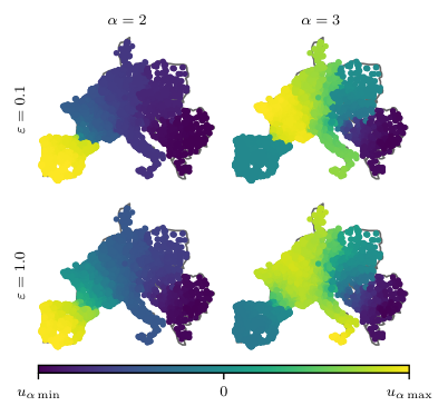
Interesting is the behavior of the fourth and fifth eigenvectors which undergo an avoided crossing shown in Fig. 3 at . Their behavior illustrates the eigenvector mixing process discussed above, as after the avoided crossing, , the actual eigenvectors are given by , where denotes the eigenvector before the avoided crossing. This results in overlaps at for both eigenvectors. The seventh eigenvector also undergoes an avoided crossing at , which mixes it with the high-lying eigenvectors. From Fig. 3 we see that this is accompanied by an abrupt decrease of . These phenomena nicely illustrate the direct connection between avoided crossings and changes in the eigenvectors structure.

Figs. 1 and 6 show that the lowest hybridized zero-mode essentially resides in the Iberian Peninsula and in the Balkans. These are two of the seven areas in our aggregation. We found that oscillations between these two areas are triggered by a perturbation in either one. This is shown in Fig. 1 in the case of a noisy power injection. The chosen noise is an Ornstein-Uhlenbeck noise with a correlation time much larger than the oscillation frequency, and we found that the latter is close to the oscillation frequencies of the two lowest hybridized zero-modes and not related to any perturbation time scale. These two modes are excited by the perturbation, and the addition of their components evidently resolves the two areas as shown in Fig. 1.
As another example, we finally investigate the reaction of the system to a 900 MW power loss. Fig. 7 shows the response of the Balkan area and the Iberian Peninsula to a fault in the opposing area. As before, all nodes within one area respond coherently – with the same frequency and phase – to a fault in the opposing area, with only moderate variations of the response amplitude. The Fourier transform of the oscillation response in the Iberian Peninsula is further shown in the bottom panel. Superimposed on it are the locations of the eigenfrequencies of the -matrix, and the Fourier spectrum indicates that only the first two eigenmodes are excited, with a broadening originating from the damping in Eq. (4). This confirms our above claim that inter-area oscillations in the PanTaGruEl network are mainly carried by the two lowest modes of the system.
V Conclusion
The standard approach to slow coherency successfully predicts the structure of slowly oscillating, long-wavelength inter-area modes, even in strongly connected power networks that lie outside its range of validity. The theory presented above puts this theory on solid grounds even in such well connected networks. Our line of reasoning goes as follows.
First, we recalled that in homogeneous systems with constant inertia and damping, small-signal oscillations in the swing equations (1) are carried by eigenmodes of the -matrix of Eq. (6). The structure of these modes is solely determined by the eigenmodes of the Laplacian matrix of the network [20].
Second, when dealing with slow coherency/inter-area oscillations, the focus is on the slowly oscillating modes. A recent extension of Courant’s nodal domain theorem [13] shows that the slow modes have large nodal domains [14]. Because of that, these slow modes are only poorly resolving inhomogeneities in inertia and damping and are therefore much less sensitive to them. Perturbation theory makes this quantitative and shows that, while in the presence of significant inhomogeneities, most eigenmodes of the -matrix acquire a structure not necessarily captured by those of the network Laplacian . The long-wavelength modes of retain the structure of the slow modes of .
Third, using perturbation theory, we showed that an appropriate choice of disaggregation of the network into initially disconnected areas captures the slow modes from the hybridization of the zero modes of each area Laplacian, even when the inter-area couplings are restored. This clarifies the origin of the slow coherency, inter-area modes, and in particular explains how they often are quasi-homogeneous over large areas – they originate from area-Laplacian zero-modes that are exactly constant there.
The aim of our theory was not to identify the optimal initial aggregation. We found numerically that standard numerical aggregation algorithms do a good job at predicting that. Our theory fills an important theoretical gap, in that it explains (i) the origin of the slow inter-area modes and (ii) why the standard approach to inter-area oscillations still works well outside its range of validity. Doing so, we closed a number of loopholes in the theory of inter-area oscillations in transmission power networks.
Acknowledgment
We are grateful to M. Tyloo for discussions at the early stage of this project and to G. Evequoz for discussions on Courant’s nodal domain theorem.
References
- [1] G. Rogers, Power System Oscillations. Boston, MA: Springer US, 2000.
- [2] V. Venkatasubramanian and Y. Li, “Analysis of 1996 western american blackouts,” in Bulk Power System Dynamics and Control - VI, Cortina d’Ampezzo, Aug. 2004, pp. 685–721.
- [3] X. Zhang, C. Lu, S. Liu, and X. Wang, “A review on wide-area damping control to restrain inter-area low frequency oscillation for large-scale power systems with increasing renewable generation,” Renewable and Sustainable Energy Reviews, vol. 57, pp. 45–58, 2016. [Online]. Available: https://www.sciencedirect.com/science/article/pii/S1364032115015506
- [4] R. Nath, S. S. Lamba, and K. P. Rao, “Coherency based system decomposition into study and external areas using weak coupling,” IEEE Transactions on Power Apparatus and Systems, vol. PAS-104, no. 6, pp. 1443–1449, Jun. 1985.
- [5] J. H. Chow, Ed., Time-Scale Modeling of Dynamic Networks with Applications to Power Systems, ser. Lecture Notes in Control and Information Sciences. Berlin/Heidelberg: Springer-Verlag, 1982, vol. 46.
- [6] R. Podmore, “Identification of coherent generators for dynamic equivalents,” IEEE Transactions on Power Apparatus and Systems, vol. PAS-97, no. 4, pp. 1344–1354, Jul. 1978.
- [7] M. Jonsson, J. Daalder, and M. Begovic, “A system protection scheme concept to counter interarea oscillations,” IEEE Transactions on Power Delivery, vol. 19, no. 4, pp. 1602–1611, Oct. 2004.
- [8] R. Date and J. Chow, “Aggregation properties of linearized two-time-scale power networks,” IEEE Transactions on Circuits and Systems, vol. 38, no. 7, pp. 720–730, Jul. 1991.
- [9] J. H. Chow, J. J. Allemong, and P. V. Kokotovic, “Singular perturbation analysis of systems with sustained high frequency oscillations,” Automatica, vol. 14, no. 3, pp. 271–279, May 1978.
- [10] M. Tyloo, L. Pagnier, and P. Jacquod, “The key player problem in complex oscillator networks and electric power grids: Resistance centralities identify local vulnerabilities,” Science Advances, vol. 5, no. 11, p. eaaw8359, Nov. 2019.
- [11] L. Pagnier and P. Jacquod, “Inertia location and slow network modes determine disturbance propagation in large-scale power grids,” PLOS ONE, vol. 14, no. 3, p. e0213550, Mar. 2019.
- [12] J. Machowski, Z. Lubosny, J. W. Bialek, and J. R. Bumby, Power System Dynamics: Stability and Control, 3rd ed. Hoboken, NJ, USA: John Wiley, 2020.
- [13] R. Courant, “Ein allgemeiner satz zur theorie der eigenfunktionen selbstadjungierter differentialausdrücke,” Nachrichten von der Gesellschaft des Wissenschaften zu Göttingen, vol. 1, pp. 80–84, 1923.
- [14] J. Urschel, “Nodal decompositions of graphs,” Linear Algebra and its Applications, vol. 539, pp. 60–71, 2018.
- [15] B. Bamieh, “A tutorial on matrix perturbation theory (using compact matrix notation),” arXiv:2002.05001, 2020.
- [16] J. Fritzsch, M. Tyloo, and P. Jacquod, “Matrix perturbation theory of inter-area oscillations,” in 2021 60th IEEE Conference on Decision and Control (CDC). IEEE, dec 2021.
- [17] A. Bergen and D. Hill, “A structure preserving model for power system stability analysis,” IEEE Transactions on Power Apparatus and Systems, vol. PAS-100, no. 1, pp. 25–35, Jan. 1981.
- [18] E. Welfonder, H. Weber, and B. Hall, “Investigations of the frequency and voltage dependence of load part systems using a digital self-acting measuring and identification system,” IEEE Transactions on Power Systems, vol. 4, no. 1, pp. 19–25, 1989.
- [19] J. O'Sullivan and M. O'Malley, “Identification and validation of dynamic global load model parameters for use in power system frequency simulations,” IEEE Transactions on Power Systems, vol. 11, no. 2, pp. 851–857, may 1996.
- [20] T. Coletta and P. Jacquod, “Linear stability and the braess paradox in coupled-oscillator networks and electric power grids,” Physical Review E, vol. 93, no. 3, p. 032222, Mar. 2016.
- [21] L. Pagnier and P. Jacquod, “Optimal placement of inertia and primary control: A matrix perturbation theory approach,” IEEE Access, vol. 7, pp. 145 889–145 900, 2019.
- [22] R. A. Horn and C. R. Johnson, Matrix Analysis, 2nd ed. Cambridge ; New York: Cambridge University Press, 2012.
- [23] J. J. Sakurai and J. Napolitano, Modern Quantum Mechanics, 2nd ed. Cambridge: Cambridge University Press, 2017.
- [24] J. Ma, T. Wang, Z. Wang, and J. S. Thorp, “Application of 2nd order matrix perturbation to compute power system inter-area oscillation modes considering uncertainties,” in 2012 IEEE Power and Energy Society General Meeting, Jul. 2012, pp. 1–6.
- [25] Y. Yang, J. Zhao, H. Liu, Z. Qin, J. Deng, and J. Qi, “A matrix-perturbation-theory-based optimal strategy for small-signal stability analysis of large-scale power grid,” Protection and Control of Modern Power Systems, vol. 3, no. 1, p. 34, Nov. 2018.
- [26] Y. Yi, A. Das, B. Bamieh, Z. Zhang, and S. Patterson, “Diffusion and consensus in a weakly coupled network of networks,” IEEE Transactions on Control of Network Systems, pp. 1–1, 2021.
- [27] F. Haake, S. Gnutzmann, and M. Kuś, Quantum Signatures of Chaos. Cham, Switzerland: Springer, 2018.
- [28] J. von Neumann and E. P. Wigner, “über das verhalten von eigenwerten bei adiabatischen prozessen,” Physikalische Zeitschrift, vol. 30, pp. 467–470, 1929.
- [29] M. Tyloo, T. Coletta, and P. Jacquod, “Robustness of synchrony in complex networks and generalized kirchhoff indices,” Physical Review Letters, vol. 120, no. 8, p. 084101, Feb. 2018.
- [30] H. Min and E. Mallada, “Dynamics concentration of large-scale tightly-connected networks,” in 2019 IEEE 58th Conference on Decision and Control (CDC). IEEE, dec 2019.
- [31] J. H. Chow, Ed., Power System Coherency and Model Reduction, ser. Power Electronics and Power Systems. New York: Springer, 2013, no. Volume 94.
- [32] D. Romeres, F. Dörfler, and F. Bullo, “Novel results on slow coherency in consensus and power networks,” in 2013 European Control Conference (ECC), Jul. 2013, pp. 742–747.
- [33] C. Grigg, P. Wong, P. Albrecht, R. Allan, M. Bhavaraju, R. Billinton, Q. Chen, C. Fong, S. Haddad, S. Kuruganty, W. Li, R. Mukerji, D. Patton, N. Rau, D. Reppen, A. Schneider, M. Shahidehpour, and C. Singh, “The ieee reliability test system-1996. a report prepared by the reliability test system task force of the application of probability methods subcommittee,” IEEE Transactions on Power Systems, vol. 14, no. 3, pp. 1010–1020, Aug. 1999.