Floquet solitons in square lattices: Existence, Stability and Dynamics
Abstract
In the present work, we revisit a recently proposed and experimentally realized topological 2D lattice with periodically time-dependent interactions. We identify the fundamental solitons, previously observed in experiments and direct numerical simulations, as exact, exponentially localized, periodic in time solutions. This is done for a variety of phase-shift angles of the central nodes upon an oscillation period of the coupling strength. Subsequently, we perform a systematic Floquet stability analysis of the relevant structures. We analyze both their point and their continuous spectrum and find that the solutions are generically stable, aside from the possible emergence of complex quartets due to the collision of bands of continuous spectrum. The relevant instabilities become weaker as the lattice size gets larger. Finally, we also consider multi-soliton analogues of these Floquet states, inspired by the corresponding discrete nonlinear Schrödinger (DNLS) lattice. When exciting initially multiple sites in phase, we find that the solutions reflect the instability of their DNLS multi-soliton counterparts, while for configurations with multiple excited sites in alternating phases, the Floquet states are spectrally stable, again analogously to their DNLS counterparts.
I Introduction
The study of topological features and their interplay with the dynamics is a theme of growing significance in a diverse variety of fields including photonics Ozawa et al. 2019, cold atom physics Cooper et al. 2019, as well as phononics Ma et al. 2019; Süsstrunk and Huber 2016 and metamaterials Deng et al. 2021, among others. While much of the relevant emphasis has been on linear features of relevant models, progressively there is an increasing number of studies at the interface between nonlinearity and topology Smirnova et al. 2020; Ma et al. 2021; see also the corresponding chapter of Kevrekidis et al. 2020.
In the context of nonlinear systems, there has been progress in a number of pertinent directions. For instance, nonlinearity has been leveraged in order to modulate the frequency and generate the harmonics of edge states Dobrykh et al. 2018; Pal et al. 2018; Vila et al. 2019; Kruk et al. 2019; Wang et al. 2019; Darabi and Leamy 2019; Zhou et al. 2020. Moreover, coherent nonlinear wave structures that are dynamically robust and potentially propagate on edges of domains in the context of models with suitable topology have been identified Ablowitz et al. 2014; Leykam and Chong 2016; Kartashov and Skryabin 2016; Snee and Ma 2019; Tao et al. 2020. Among the numerous further states that have been explored, one can mention nonlinear Dirac cones Bomantara et al. 2017, gap solitons induced by topological bands Lumer et al. 2013; Solnyshkov et al. 2017; Smirnova et al. 2019; Marzuola et al. 2019; Mukherjee and Rechtsman 2020, as well as domain walls Chen et al. 2014; Hadad et al. 2017; Poddubny and Smirnova 2018. Features such as the uninhibited unidirectional, scatter-free (around lattice defects) propagation of nonlinear edge modes in topological lattices (such as Lieb, Kagomé etc.) Ablowitz and Cole 2019, as well as the absence of Peierls-Nabarro, discreteness-induced barriers in nonlinear Floquet topological insulators Ablowitz et al. 2021 have been manifested. These suggest the particular promise of topological nonlinear media in overcoming some of the limitations of “conventional” nonlinear modes. Recently, relevant topological phase transitions have been extended to entire soliton lattices Bongiovanni et al. 2021.
In the present work, our aim is to explore systematically a model of an anomalous Floquet topological insulator that has not only been recently proposed, but also experimentally implemented in Mukherjee and Rechtsman 2020. In the relevant context, a periodically modulated waveguide lattice was produced, with the Floquet (periodic) driving inducing a nonvanishing winding number. This, in turn, was argued to produce topological edge modes in the relevant spectrum. The topological bandgap produced in such a medium, in the presence of cubic nonlinearity due to the optical Kerr effect, was found to lead to the formation of solitary waves that could be experimentally observed in Mukherjee and Rechtsman 2020. While such waves were identified and the extent of their spatial localization was examined for different input powers in this work, an understanding of such states is still rather limited from the nonlinear and dynamical systems point of view.
Here, we offer a systematic exploration of the existence and stability of such states. Imposing a Floquet, time-periodic modulation of the waveguide coupling emulating that of the experiment, we seek and are able to identify such states as numerically exact solutions, up to a prescribed numerical accuracy. This is done for a variety of phase-shifts arising for each period of the coupling modulation (such as, e.g., , , etc.), extending in this way the direct simulations and experiments of Mukherjee and Rechtsman 2020. Once the relevant waveforms have been identified, a natural subsequent question is that of their dynamical stability. The experimental observation of such states predisposes towards their stability and hence observability, yet the parametric range of such a feature is of particular interest. Indeed, here we report a systematic Floquet analysis which reveals that the relevant fundamental states are spectrally stable, featuring multipliers purely on the unit circle for wide parametric intervals. Interestingly, the relevant spectrum is found to consist of a continuous spectrum surrounding in the Floquet multiplier plane, and of a few point-spectrum multipliers associated with the excitations of the core of the relevant solitary wave. Instabilities emerge as a byproduct of the finite size of the numerical computations and have been dynamically monitored, yet relevant features of the continuous spectrum are found to weaken for progressively larger lattices and hence are expected to be absent in the infinite lattice limit. Finally, another question that stems from a well-rounded understanding of the corresponding non-time-modulated analogue of the model, namely the discrete nonlinear Schrödinger (DNLS) equation Kevrekidis 2009, is whether additional coherent structures may exist in such a setting. Indeed, here we illustrate a systematic prescription to produce multi-soliton states, which is motivated from the corresponding multi-soliton states of the DNLS. In particular, we show that an initial excitation of multiple sites (adjacent or diagonally) produces a corresponding multi-site Floquet topological soliton. Furthermore, the stability structure of the DNLS is found to carry over to the temporally modulated coupling model: in-phase excited sites are associated with a real pair of Floquet multipliers. On the other hand, out-of-phase excited states, the so-called twisted modes, are associated with a stable Floquet spectrum and long-lived multi-soliton periodic orbits. All of the above results have been corroborated by systematic numerical simulations.
The presentation of our results is structured as follows. In section 2, we discuss the model and the specific choices of initial and boundary conditions, as well as the concrete temporal modulation of the coupling. In section 3, we explore the fundamental breather states of the lattice inspired by (and substantially extending the results of) Mukherjee and Rechtsman 2020. In section 4, we leverage the detailed understanding of the DNLS model to extend considerations to multi-peak Floquet solitons and to examine their stability properties. Finally, in section 5, we summarize our findings and present some directions for future study.
II Mathematical model
The propagation of light through an optical lattice with nearest-neighbor coupling in the presence of a third-order Kerr nonlinearity can be described by the discrete nonlinear Schrödinger equation
| (1) |
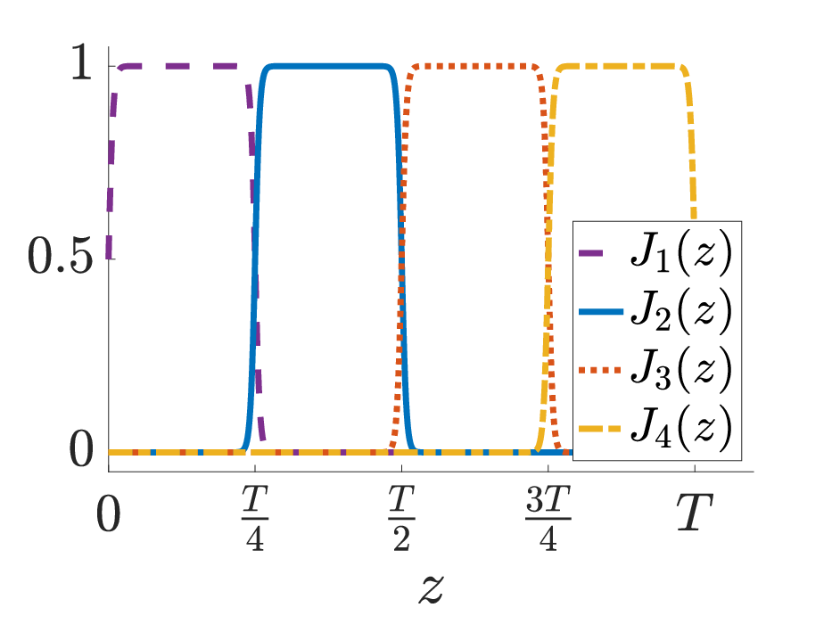
where is the coupling strength, is the strength of the nonlinearity, which we will always take to be 1. This non-dimensional version represents experimental conditions for nonlinear modes of milliwatts peak power and millimeter effective nonlinear length (that is, the non-dimensional intensity ) Mukherjee and Rechtsman 2020. is the linear tight-binding, nearest-neighbor coupling, which depends on the propagation distance Mukherjee and Rechtsman 2020 (and has an explicit form shown in Eqs. 2 below). The summation is over nearest neighbors only. We consider here a square lattice of waveguides in which the strengths of the nearest-neighbor couplings vary periodically in with fundamental period in such a way that for each , every waveguide only interacts with one of its four neighbors (Fig. 1(a)). For the two-dimensional integer lattice , equation Eq. 1 becomes
| (2) | ||||
The functions model the switching of neighbor coupling as follows. For period , we define the smoothed bump function
| (3) |
where the parameter quantifies the steepness of the bump, with steepness increasing with . The four coupling functions in Fig. 1 are then given by , , , and . Notice that effectively on any propagation distance interval of length , there is only one active coupling in place (see Figure 1b).

III Fundamental breather
The system Eq. 1 has a fundamental breather solution in which the optical intensity is localized in a square of four lattice sites (which we call the fundamental unit square) and rotates counterclockwise around these sites (Fig. 2(a) and (b)). After one period , the solution reproduces itself except for a phase shift . Numerical simulations demonstrate that this solution can be found with phase shifts of , , , and , but is not possible. (Numerical simulations suggest that solutions for for integers can be obtained, but this was practically found to be increasingly more difficult to do using a shooting method for larger .) In line with the original work of Mukherjee and Rechtsman 2020, the phase is associated with a quasi-energy resonant with the linear band of extended excitations and hence is not possible. The overall period of the breather is then given by , where is the number of periods needed to return to the starting condition. We will consider herein only the phase shifts and , but will briefly comment on what occurs in the other cases.
We use a shooting method to construct a breather solution numerically. We first choose the period and the phase shift . For all of our simulations, we will use a period of the coupling time-dependence. If , for example, the overall period of the breather will be . Starting with an initial guess , we evolve the solution forward using a 4th order Runge-Kutta scheme. To obtain a solution with period and phase shift , we iteratively solve . We also compute the Floquet spectrum of the breather solution by determining the eigenvalues of the monodromy matrix over one full breather period . For efficiency of computation, we run the simulation on a lattice with periodic boundary conditions. For the fundamental breather, a single lattice site is excited for the initial guess.
III.1 Phase shift
First, we consider the case when the phase shift is given by . Fig. 2(a) and Fig. 2(b) show the fundamental breather solution for coupling strength and phase shift , which is exponentially localized at the four central sites of the lattice. The Floquet spectrum for is located on the unit circle (relative error less than ), which suggests that this solution is stable. There is a small continuous spectrum band near on the unit circle (bottom inset in Fig. 2(c)); as the steepness parameter of the coupling functions increases, the continuous spectrum band for approaches a single point at . We explore this in Appendix A, which presents a relevant discussion as we approximate by step functions. In addition, there is a set of four isolated Floquet eigenmodes (top inset in Fig. 2(c), as well as Fig. 3(a)), together with their complex conjugates. These isolated modes are spatially localized (Fig. 2(d)), as opposed to the nonlocalized continuous spectrum modes.
Let be the continuous spectrum band, which we compute using the method described in Appendix A; this agrees with the spectrum determined by computing the eigenvalues of the monodromy matrix. Using this method, we verify numerically that has the following properties:
- (i)
(explained by the invariance in equation Eq. 4).
- (ii)
, where is the fundamental frequency of the system.
- (iii)
For , , where (Fig. 4(b)). This extends periodically in with period for outside this interval. The band is filled out as the lattice size increases, and is a continuum for the limiting lattice .
In particular, since the continuous spectrum band is a single point at when , it follows from the -periodicity of the bands that they collapse into a single point at (in the limiting case when the coupling functions are step functions) whenever is an integer multiple of . This explains what occurs at in Fig. 2(c).


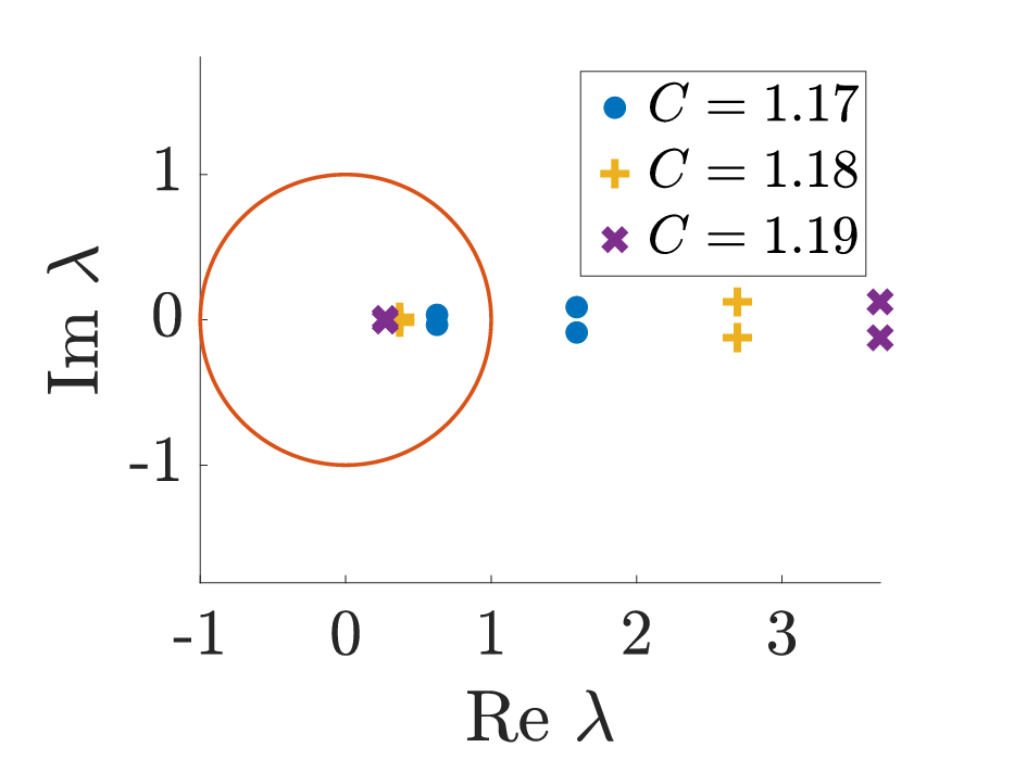
Using parameter continuation, we can compute solutions for other values of by gradually increasing (or decreasing) (Fig. 4(a)). It is relevant to note here that in the experimental setting of interest Mukherjee and Rechtsman 2020, by controlling the separation between waveguides during the fabrication process, it is, in principle, possible to control the lattice spacing, and, accordingly, to enable the manifestation of the dynamical features reported herein. As is increased from 1, some Floquet multipliers in the continuous spectrum band collide and leave the unit circle (Fig. 5(a) and Fig. 5(b)). In particular, we see from Fig. 5(a) that the isolated modes are not involved in these collisions. Although the Floquet multiplier with maximum absolute value increases with , the rate of growth decreases as the lattice size increases (Fig. 5(c)); the latter suggests that this type of instability disappears in the infinite lattice limit, in line, e.g., with what is known from the classic work of Marín and Aubry 1998. We can see the consequences of this unstable Floquet eigenmode by perturbing the fundamental breather with a small multiple of the eigenfunction corresponding to the largest Floquet multiplier (Fig. 5(d)). The slope of the least squares regression line in the figure is within 2% of , where is the largest Floquet multiplier, confirming the results of our spectral stability analysis. At longer times, the solution continues to slowly deviate from the unstable initial condition, yet does not settle into a clearly discernible pattern for the interval of our numerical computations.


Long-term evolution numerical experiments provide further evidence that the fundamental breather solution is stable for and close to 1. As an initial condition, we start with all the intensity confined to a single lattice site. The magnitude of this intensity is chosen to be the maximal intensity of the fundamental breather. Results of this evolution for , , and are shown in Fig. 6. For larger values of , this initial condition is found to disperse over longer intervals of evolution in (Fig. 6(d)). This effect persists with larger lattice sizes.


III.2 Phase shift
Next, we consider the case when the phase shift is , in which case the breather period is . When , numerical simulations, both from spectral computations and evolution experiments, suggest that the fundamental breather solution is stable. The behavior is qualitatively the same as when . However, when is increased from 1 by parameter continuation (Fig. 4), an unstable Floquet eigenmode appears at a critical value of (between and for our chosen parameters; see Fig. 7(a)). This unstable eigenmode is not on the real axis, i.e. it corresponds to a complex quartet (see inset in Fig. 7(a), as well as Fig. 7(b), which shows the growth of this mode in ), and it does not depend on the size of the grid (in contrast with what occurs for ). Its spatial profile is shown in Fig. 8(a). In addition, the unstable mode is not part of the continuous spectrum, in that it is not present in the linearization about the background state. Once again, we can see the consequences of this unstable Floquet eigenmode by perturbing the fundamental breather through adding a small multiple of the corresponding eigenfunction (Fig. 8(b)). The slope of the least squares regression line in the figure is within 2% of , where is the unstable Floquet multiplier. The log power spectrum of a single central site in the unperturbed and perturbed fundamental breather is shown in Fig. 9. While in both cases the fundamental frequency is the rotation frequency , it is evident that the unstable regime leads to a genuinely distinct evolution at longer times that involves the excitation of each node (via multiple intensity peaks) throughout the period, as is clear from the left panels of the figure. The right panels also show a discernibly distinct (and much faster in its decay) tail of the frequency dependence of the intensity. A closer inspection of the relevant spectrum over a narrow frequency range reveals the growth of sidebands which is in line with the apparent quasi-periodic behavior observed in Fig. 9(c).



III.3 Other phase shifts
Numerical computations suggests that the fundamental breather solution exists for phase shifts of and . However, in both of these cases, computation of the Floquet spectrum for shows the presence of an unstable Floquet multiplier on the real axis, hence we do not further pursue such waveforms herein.
IV Two-site breathers on the unit square
Multi-breather solutions can be found for which the initial intensity is localized at more than one site in the lattice. Here, in line with the discussion in the Supplemental Material of Mukherjee and Rechtsman 2020, we envision a scenario whereby light is launched initially on two waveguides rather than a single one. We will consider here two-site breathers, in which the initial intensity is localized at a pair of sites within the fundamental unit square. For all of these solutions, we will take . There are two possibilities for these two-site breathers, in terms of location: adjacent (sites 1 and 2 in Fig. 2) and diagonal (sites 1 and 3 in Fig. 2). In addition, for each of the two-site breather possibilities, there are two scenarios in terms of the relative phase between the sites. If the two sites are initialized in-phase, there is a Floquet eigenvalue outside the unit circle, thus this solution is unstable. If the two sites are initialized out-of-phase, the Floquet eigenvalues all lie on the unit circle (for close to 1), which suggests that this solution is stable. (See figures Fig. 10(b) and Fig. 11(b)). Of course, as is well documented for their DNLS analogues Kevrekidis 2009, as is increased such structures can eventually become unstable through complex instabilities due to multiplier quartets.
We consider the diagonal breather first, in which the initial intensity is localized at two diagonally opposite sites in the fundamental unit square (sites 1 and 3 in Fig. 10). Due to the nature of the coupling, since each is only connected to a single neighboring site for a given , the two components of the breather practically act independently. Over one period, the initial intensity at site 1 rotates counterclockwise around the fundamental unit square (sites 1,2,3,4 in Fig. 10). Since the edge between sites 3 and 5 is also active at (see Fig. 1), the initial intensity at site 3 rotates counterclockwise around the unit square located one position to the northeast (sites 3,5,6,7 in Fig. 10). Since site 3 is shared between both components of the multi-breather, its frequency is twice that of the other sites (Fig. 10(c) and Fig. 10(d)).
For the adjacent breather, the initial intensity is localized at two adjacent sites in the fundamental unit square (sites 1 and 2 in Fig. 11). The initial intensity at site 1 rotates counterclockwise around the fundamental unit square as before (sites 1,2,3,4 in Fig. 11). Since the only active connection involving site 2 at is that between sites 2 and 1 (see Fig. 1), the initial intensity at site 2 also rotates counterlockwise around the unit square located one position to the south (sites 2,1,5,6 in Fig. 11). This means that sites 1 and 2 are active for the first half of the period (Fig. 11(c)).
In both cases, if the two sites are initialized in-phase, there is a Floquet eigenvalue outside the unit circle; this eigenvalue is much larger for the adjacent breather than for the diagonal breather. If the two adjacent sites are initialized with opposite phases, the Floquet spectrum lies on the the unit circle (for close to 1). The Floquet eigenfunctions corresponding to the largest Floquet multiplier for both the unstable diagonal breather and unstable adjacent breather are shown in Fig. 12.


For the unstable adjacent two-site breathers, we can see how perturbations evolve by adding a small amount of the unstable Floquet eigenfunction to the initial condition (see Fig. 11(d)). The slope of the least squares linear regression line is 0.2783, which is a relative error of less than from the predicted value of , where is the value of the largest Floquet multiplier, and is the period of the breather. Similar results can be obtained for the unstable opposite two-site breather.
Long-term evolution numerical experiments confirm these results, and provide evidence that the diagonal breather with opposite sites initialized out-of-phase is dynamically robust (for the parameter range and propagation distance considered herein). For the initial condition, we take two diagonally opposite sites in the unit square which have the same intensities, but are out of phase by . This initial amplitude is chosen to be the maximum amplitude of the diagonal breather. Results of this evolution are shown in Fig. 13(a). Similarly, the diagonal breather with opposite sites initialized in-phase is unstable, although it takes many steps for a perturbation of this solution to break apart and lead to a distinct nearly periodic orbit, as indicated in Fig. 13(b). Similarly, numerical evolution experiments for the adjacent breather confirm that it is stable for the out-of-phase configuration (Fig. 14(a)) and unstable for the in-phase configuration (Fig. 14(b)). In fact, the instability of the adjacent breather with in-phase initialization manifests itself in a way such that it breaks apart by .


V Conclusions & Future Challenges
In the present work, we have explored a wide set of Floquet solitary wave structures in a system bearing a topological bandgap. In particular, we were motivated by direct numerical simulations and experimental observations in a photonic implementation of system with waveguides bearing a time-modulated coupling structure in two spatial dimensions. We were able to identify prototypical time-periodic solutions of the system in the form of fundamental breathers bearing different phase shifts upon completion of a period of the time variation of the coupling. We analyzed the Floquet spectrum of such solitons, distinguishing their continuous spectrum (and its dependence on the coupling parameter), as well as the point spectrum associated with the excited sites of the relevant coherent structure. We found that, aside from lattice-size-dependent oscillatory instabilities, the fundamental breathers were spectrally, as well as dynamically robust. We then moved one step further, exploring multi-peak (excited) structures. We leveraged a detailed understanding of the spectral picture of such structures in the stationary DNLS limit to explain the corresponding stability analysis of excited, multi-peaked time-periodic states. In particular, we found that double-peaked states are unstable if the two sites are initialized in-phase, and spectrally stable if the two sites are initialized out-of-phase. This relationship between phase and stability is similar to what is observed for multi-peaked standing wave solutions in DNLS lattices, both in one and two dimensions Kalosakas 2006; Parker et al. 2020, as well as breather solutions in Klein-Gordon lattices Pelinovsky and Sakovich 2012.
Naturally, this is not a full outcome in this ongoing effort to explore the existence, stability and dynamical properties of topological solitonic structures. For instance, one can consider different types of lattices, including Lieb and Kagomé ones, and further explore the wave patterns that arise therein and their corresponding spectra. Another aspect in which topological features may have a strong imprint is the mobility of nonlinear modes. Indeed, it has been argued in recent works, including Ablowitz and Cole 2019; Ablowitz et al. 2021; Mukherjee and Rechtsman 2021, that topology may control and, indeed, even enhance (when suitably leveraged) the mobility of states that might not be otherwise particularly mobile (e.g., due to Peierls-Nabarro and associated barriers Kevrekidis 2009; Ablowitz et al. 2021) in conventional discrete settings. It is intriguing to consider if mobility of photonic modes can be achieved in a similar way to what is seen in the propagation of nonlinear elastic waves in flexible structures which provides opportunities for locomotion of mechanical robots Deng et al. 2020. Having focused herein on stationary states, such features are worthwhile of further exploration and we defer corresponding studies to future publications.
Acknowledgements.
This material is based upon work supported by the U.S. National Science Foundation under the RTG grant DMS-1840260 (R.P. and A.A.), DMS-1809074 (P.G.K.), and DMS-1909559 (A.A.). J.C.-M. acknowledges support from EU (FEDER program 2014-2020) through both Consejería de Economía, Conocimiento, Empresas y Universidad de la Junta de Andalucía (under the projects P18-RT-3480 and US-1380977), and MICINN and AEI (under the projects PID2019-110430GB-C21 and PID2020-112620GB-I00).Appendix A Continuous spectrum bands
We compute the continuous spectrum bands in the limiting case where the coupling functions are step functions. We note that although these step functions are not everywhere differentiable, we can treat the -dependent term in Eq. 1 as piecewise constant. First, we linearize equation Eq. 1 about the solution , which is equivalent to only considering the linear terms. We then take the Floquet ansatz , where is periodic in with period , and . Substituting this into Eq. 1 and simplifying, we obtain the sequence of equations
| (4) |
for , which is extended periodically for all . The are piecewise constant linear operators which implement the lattice couplings in Fig. 1(a). When , the only solutions with period are when is an integer multiple of , which implies that there is a single Floquet multiplier at with infinite multiplicity. Over one period , the solution to Eq. 4 is given by
| (5) |
where
| (6) |
We note that the exponentials in this product do not commute, since the operators do not commute. For to be in the continuous spectrum, we require , i.e. the operator on the RHS of Eq. 5 must be the identity. This is equivalent to
| (7) |
thus the Floquet multipliers are exactly the eigenvalues of .
We can compute these by approximating the integer lattice with successively larger finite lattices. For a square lattice of size , with periodic boundary conditions imposed on the couplings, the operators are represented by symmetric adjacency matrices. Computing the eigenvalues of numerically, we verify properties (i)-(iii) of the continuous spectrum in Section III.1. These results do not depend on how the lattice points are arranged in the adjacency matrices .
References
- Ozawa et al. (2019) T. Ozawa, H. M. Price, A. Amo, N. Goldman, M. Hafezi, L. Lu, M. C. Rechtsman, D. Schuster, J. Simon, O. Zilberberg, and I. Carusotto, Rev. Mod. Phys. 91, 015006 (2019).
- Cooper et al. (2019) N. R. Cooper, J. Dalibard, and I. B. Spielman, Rev. Mod. Phys. 91, 015005 (2019).
- Ma et al. (2019) G. Ma, M. Xiao, and C. T. Chan, Nat. Rev. Phys. 1, 281 (2019).
- Süsstrunk and Huber (2016) R. Süsstrunk and S. D. Huber, Proc. Natl. Acad. Sci. USA 113, E4767 (2016).
- Deng et al. (2021) B. Deng, J. Li, V. Tournat, P. K. Purohit, and K. Bertoldi, Journal of the Mechanics and Physics of Solids 147, 104233 (2021).
- Smirnova et al. (2020) D. Smirnova, D. Leykam, Y. Chong, and Y. Kivshar, Appl. Phys. Rev. 7, 021306 (2020).
- Ma et al. (2021) Q. Ma, A. Grushin, and K. Burch, Nat. Mater. 10.1038/s41563-021-00992-7 (2021).
- Kevrekidis et al. (2020) P. G. Kevrekidis, J. Cuevas-Maraver, and A. Saxena, Emerging Frontiers in Nonlinear Science, 1st ed. (Springer Nature, Heidelberg, 2020).
- Dobrykh et al. (2018) D. A. Dobrykh, A. V. Yulin, A. P. Slobozhanyuk, A. N. Poddubny, and Y. S. Kivshar, Phys. Rev. Lett. 121, 163901 (2018).
- Pal et al. (2018) R. K. Pal, J. Vila, M. Leamy, and M. Ruzzene, Phys. Rev. E 97, 032209 (2018).
- Vila et al. (2019) J. Vila, G. H. Paulino, and M. Ruzzene, Phys. Rev. B 99, 125116 (2019).
- Kruk et al. (2019) S. Kruk, A. Poddubny, D. Smirnova, L. Wang, A. Slobozhanyuk, A. Shorokhov, I. Kravchenko, B. Luther-Davies, and Y. Kivshar, Nat. Nanotechnol. 14, 126 (2019).
- Wang et al. (2019) Y. Wang, L.-J. Lang, C. H. Lee, B. Zhang, and Y. D. Chong, Nat. Commun. 10, 1102 (2019).
- Darabi and Leamy (2019) A. Darabi and M. J. Leamy, Phys. Rev. Applied 12, 044030 (2019).
- Zhou et al. (2020) D. Zhou, J. Ma, K. Sun, S. Gonella, and X. Mao, Phys. Rev. B 101, 104106 (2020).
- Ablowitz et al. (2014) M. J. Ablowitz, C. W. Curtis, and Y.-P. Ma, Phys. Rev. A 90, 023813 (2014).
- Leykam and Chong (2016) D. Leykam and Y. D. Chong, Phys. Rev. Lett. 117, 143901 (2016).
- Kartashov and Skryabin (2016) Y. V. Kartashov and D. V. Skryabin, Optica 3, 1228 (2016).
- Snee and Ma (2019) D. D. Snee and Y.-P. Ma, Extreme Mech. Lett. 30, 100487 (2019).
- Tao et al. (2020) Y.-L. Tao, N. Dai, Y.-B. Yang, Q.-B. Zeng, and Y. Xu, arXiv:2005.04433 (2020).
- Bomantara et al. (2017) R. W. Bomantara, W. Zhao, L. Zhou, and J. Gong, Phys. Rev. B 96, 121406(R) (2017).
- Lumer et al. (2013) Y. Lumer, Y. Plotnik, M. C. Rechtsman, and M. Segev, Phys. Rev. Lett. 111, 243905 (2013).
- Solnyshkov et al. (2017) D. D. Solnyshkov, O. Bleu, B. Teklu, and G. Malpuech, Phys. Rev. Lett. 118, 023901 (2017).
- Smirnova et al. (2019) D. A. Smirnova, L. A. Smirnov, D. Leykam, and Y. S. Kivshar, Laser Photonics Rev. 13, 1900223 (2019).
- Marzuola et al. (2019) J. L. Marzuola, M. Rechtsman, B. Osting, and M. Bandres, arXiv:1904.10312 (2019).
- Mukherjee and Rechtsman (2020) S. Mukherjee and M. C. Rechtsman, Science 368, 856 (2020).
- Chen et al. (2014) B. G.-g. Chen, N. Upadhyaya, and V. Vitelli, Proc. Natl. Acad. Sci. USA 111, 13004 (2014).
- Hadad et al. (2017) Y. Hadad, V. Vitelli, and A. Alu, ACS Photon. 4, 1974 (2017).
- Poddubny and Smirnova (2018) A. N. Poddubny and D. A. Smirnova, Phys. Rev. A 98, 013827 (2018).
- Ablowitz and Cole (2019) M. J. Ablowitz and J. T. Cole, Phys. Rev. A 99, 033821 (2019).
- Ablowitz et al. (2021) M. J. Ablowitz, J. T. Cole, P. Hu, and P. Rosenthal, Phys. Rev. E 103, 042214 (2021).
- Bongiovanni et al. (2021) D. Bongiovanni, D. Jukić, Z. Hu, F. Lunić, Y. Hu, D. Song, R. Morandotti, Z. Chen, and H. Buljan, Phys. Rev. Lett. 127, 184101 (2021).
- Kevrekidis (2009) P. Kevrekidis, The discrete nonlinear Schrödinger Equation, 1st ed. (Springer-Verlag, Heidelberg, 2009).
- Marín and Aubry (1998) J. Marín and S. Aubry, Physica D 119, 163 (1998).
- Kalosakas (2006) G. Kalosakas, Physica D: Nonlinear Phenomena 216, 44 (2006), nlin/0512028 .
- Parker et al. (2020) R. Parker, P. Kevrekidis, and B. Sandstede, Physica D: Nonlinear Phenomena 408, 132414 (2020).
- Pelinovsky and Sakovich (2012) D. Pelinovsky and A. Sakovich, Nonlinearity 25, 3423 (2012).
- Mukherjee and Rechtsman (2021) S. Mukherjee and M. C. Rechtsman, Phys. Rev. X (accepted) (2021).
- Deng et al. (2020) B. Deng, L. Chen, D. Wei, V. Tournat, and K. Bertoldi, Science Advances 6, eaaz1166 (2020).