The Effects of Cosmic-Ray Diffusion and Radiative Cooling on the Galactic Wind from the Milky WayJournal: ApJCloudy (Ferland et al. 2017)
Abstract
The effects of cosmic-ray diffusion and radiative cooling on the structure of the Galactic wind are studied using a steady state approximation. It is known that realistic cooling processes suppress the wind from launching. The effects of cosmic-ray diffusion are also supposed to be unfavorable for launching the wind. Both of these effects have not been studied simultaneously in a steady-state approximation of the wind. We find 327,254 solutions of the steady-state Galactic wind and confirm that: the effect of cosmic-ray pressure depends on the Alfvén Mach number, the mass flux carried by the wind does not depend on the cosmic-ray pressure directly (but depends on the thermal pressure), and the typical conditions found in the Galaxy may correspond to the wind solution that provides metal polluted matters at a height of kpc from the disk.
Keywords:
Galactic winds — Galactic cosmic rays — Star formation — Milky Way evolutionI Introduction
Supernovae inject momenta, energies, and cosmic-rays (CRs) into the interstellar medium (ISM). These drive the dynamics of ISM (McKee & Ostriker 1977, e.g.,) and eventually result in the cloud formation (Inutsuka et al. 2015). The dynamics of ISM are controlled by the pressures of thermal gas, turbulence, CRs, and magnetic fields, which are comparable to each other (Boulares & Cox 1990; Ferrière 2001). The Galactic archaeological study shows that the overall star formation rate in the Galaxy did not deviate much in the past Gyr (Haywood et al. 2016, e.g.,). In this paper, we study this nonobvious star formation history in terms of the mass budget of gaseous matter in the Galaxy.
The star formation rate of the Milky Way (MW), , indicates a depletion of all gaseous matter in the Galactic disk with a mass of within a time of Gyr (Kennicutt & Evans 2012, e.g.,). Therefore, to understand the star formation history of the MW, which has been maintained during Gyr with almost constant rate, we must study the replenishment mechanisms of the gaseous matter. Recent observations of metal absorption lines (e.g., Mg II, O VI, etc.) around external galaxies suggest that the circumgalactic medium (CGM) is huge mass reservoir with a mass of (e.g., Tumlinson et al. 2017, and refernces therein). Since these absorption lines are ubiquitously observed around the host galaxy with a distance more than kpc, we may naturally consider the galactic wind as a metal transfer mechanism. Once the wind is really driven, the metal-polluted CGM cools significantly by the radiative cooling and eventually falls to the host galaxy. Thus, we have to study the possible conditions to launch such outflow that is a part of the mass cycle, like a galactic fountain flow (Shapiro & Field 1976) but with a scale height of kpc.
Shapiro & Field 1976 suggested the galactic fountain flow based on observations of O VI absorption lines in our Galaxy. Note that for the case of our galaxy, locations of gas responsible for the absorption lines are still not constrained observationally (Bregman & Lloyd-Davies 2007, e.g.,). Comparison the radiative cooling rate to the reheating rate of gas by supernovae, the galactic fountain flow is considered to have a scale height of kpc. Breitschwerdt et al. 1991 considered that hot, tenuous gas coexisting with the cool, condensed fountain flow is pushed by the CR pressure and eventually escapes from the Galaxy as the Galactic wind. They showed steady-state solutions without radiative cooling, diffusion of CRs, and other possible heating process. 11 1 However, they studied the effects of Alfvén wave damping using the model of Ipavich 1975, which treats the Galactic system with a spherical geometry acting as a point source of mass and energy at the center. Their main analysis was done by using a model in cylindrical coordinates (the Galactic disk model) without the wave damping. Radiative cooling was introduced by Breitschwerdt & Schmutzler 1999, but the diffusion of CRs was neglected. Recchia et al. 2016 introduced the CR diffusion and heating due to the dissipation of Alfvén waves, but they did not consider the radiative cooling. Note that they solved the CR spectrum differing from other studies and showed that the net CR pressure is almost the same as that calculated by the fluid approximations. Thus, we study steady-state outflow solutions including the radiative cooling, CR diffusion, and heating due to the wave dissipation with fluid approximations.
Recent numerical simulations study the dynamical role of CRs in launching the Galactic wind (Girichidis et al. 2018; Hopkins et al. 2018, e.g.,). Girichidis et al. 2018 investigated outflows launched from the midplane of the Galactic disk with solar neighborhood conditions using a local box approximation with a size of 0.5 kpc 0.5 kpc kpc. They found that the CR pressure can efficiently support the launching outflows and strongly affects their phase structure. Their analysis was concentrated at a height of kpc from the midplane. Hopkins et al. 2018 performed a global simulation in the context of galaxy formation and showed that the CR pressure can drive the Galactic wind (outflow with a height of kpc) for the conditions of their simulated galaxy. In their simulation, the inflow is also seen. These results may not be so surprising in qualitatively because CRs do not lose their energy compared with the thermal gas; the additional pressure can affect the thermal gas. The aim of this paper is to show the effect of the CR pressure explicitly by analyzing steady state-solutions of the outflow.
This paper is organized as follows. In Sect. II, we provide a physical model of the Galactic wind. In Sect. III, the wind equation is analyzed, and the role of CRs is discussed. The solutions of the Galactic wind are shown in Sect. IV. Finally, we summarize our results and discuss future prospects in Section V.
II Physical Model

We study a steady outflow taking into account the effects of the CRs. Figure 1 shows the model geometry. We approximate that the Galactic disk to be axially symmetric and work in cylindrical coordinates. The radial distance of the disk is , and the distance perpendicular to the disk is . There is hot gaseous layer above the Galactic disk with a thickness of several kpc that may be created due to supernova explosions (Lockman 1984; Girichidis et al. 2018, the so called Lockman layer;). The outflow is solved from kpc for the range of in this paper.
Plasma escaping from the galaxy may have a temperature comparable to the virial temperature. Therefore, we presume that the gas within the Lockman layer has a temperature comparable to the virial temperature of the MW for a radius of , , and has a number density of . The existence of gas with such temperature and density at is implied by X-ray observations (Nakashima et al. 2018, e.g.,) and numerical simulations (Girichidis et al. 2018, e.g.,). Supposing a magnetic field with a strength of , we estimate the plasma- as , where , , and are the mean molecular weight, number density, and temperature, respectively. Thus, the dynamics of the outflow may not be affected by the magnetic field that may be along the direction of travel of the outflow. We assume that the magnetic field is always along with the flow in this paper.
Since the geometry of the MW is that of a thin disk with assuming the axial symmetry, the outflow ‘feels’ the gravitational acceleration approximately along the vertical direction at a relatively small height. Thus, we treat a one-dimensional outflow traveling along the -direction so that the required energy for launching the outflow becomes approximately minimum. When the outflow reaches a height comparable with the size of the Galactic disk, it feels a more multidimensional (i.e., spherical) gravitational acceleration. At such height, the outflow should cross a surface element like that of the spherical coordinate. Hence, following Breitschwerdt et al. 1991, we assume that the outflow travels along a cylindrical flux tube given by
| (1) |
where is the area cross section of the flux tube at , whose actual value is not important in this paper. The transition scale from vertical to spherical is represented by . Along this flux tube, the divergence and gradient operations are represented by
| (2) |
Thus, the mass and magnetic fluxes are given by
| (3) | |||
| (4) |
so that const. and const. where and are the mass density and velocity of the fluid, respectively.
The outflow mainly consists of nonrelativistic, thermal particles that are forced by the pressures of the CRs and Alfvén waves. The basic equations (equation of motion and energy fluxes) of this system can be given by (Breitschwerdt et al. 1991, see),
| (5) | |||
| (6) | |||
| (7) | |||
where , ,and are the pressure, Alfvén speed, and the adiabatic index of the thermal particles, respectively. The gravitational acceleration due to the stars in the galaxy and dark matter halo is , as given in the Sect. II.1. The pressures of the CRs and Alfvén waves, and , are taken into account for the gas dynamics so that they appear in the equation of motion (5). Equations (II) and (II) describe the transport of the CRs and energy density of Alfvén waves, respectively, where is the spatial diffusion coefficient of the CRs, and is the adiabatic index for relativistic particles. These sets of equations were derived previously, e.g., by Achterberg 1981a. The dissipation of Alfvén waves is represented by , which results in the heating of the thermal particles (discussed in the Sect. II.2). is the radiative cooling function for the thermal particles and is given in the Sect. II.3. Here, we omit the hadronic losses of the CRs that are inefficient in the tenuous medium.22 2 The collision time of the CRs via hadronic interactions can be estimated as where and are the speed of light and the cross section of the hadronic interaction, respectively.
II.1 Gravitational Acceleration
For the gravitational potential formed by the stars in the Galactic bulge and disk, Miyamoto & Nagai 1975 gave a convenient pair of functions in the cylindrical coordinates as
| (9) |
where the gravitational constant is , and the fit parameters are kpc, kpc, and for the bulge and disk, respectively.
For the dark matter halo, we assume a Navarro-Frenk-White (NFW)-like density profile (Navarro et al. 1996) as
| (10) |
where the dark matter density is , the normalized galactocentric radius is , and the parameters and characterize the total mass and extent of the dark matter halo, respectively. The gravitational acceleration of the dark matter halo is obtained from the Poisson equation,
| (11) |
as
| (12) |
where the total mass of the dark matter halo is
| (13) |
Setting the parameters as , , and (Sofue 2012, e.g.), we obtain the core radius as kpc.
The total gravitational acceleration is written as
| (14) |
and is represented by Figure 2 for (top panel) and (bottom panel).


II.2 Interplay between the Cosmic Rays and Alfvén Waves
The CRs can excite the Alfvén waves in the background plasma (Lerche 1966; Lerche 1967; Wentzel 1968; Kulsrud & Pearce 1969). In the fluid approximation of CRs, the generation rate of the wave can be estimated as (Kulsrud 2005, e.g.,) and appears on the right-hand side of Eqs. (II) and (II) as the energy sink and source term, respectively. Note that .
On the other hand, the Alfvén waves in a high -plasma can be dissipated via (at least) the nonlinear Landau damping (Lee & Völk 1973; Achterberg 1981b). We assume a local equilibrium between the wave generation and dissipation so that the energy sink term of the wave energy in Eqs. (II), , is equal to (Volk & McKenzie 1981; Zirakashvili et al. 1996). The dissipated energy is converted to the thermal energy of gas; therefore appears on the right-hand side of Eq. (II) as the heating term.
CRs are scattered by the Alfvén waves, which results in the diffusion of the CRs. The actual diffusion coefficient of the CRs currently remains to be uncertain. We assume one of the most frequently invoked coefficients that is estimated from the observations of CR compositions (see Hayakawa et al. 1958; Ginzburg & Syrovatskii 1964; Gabici et al. 2019, for a recent review),
| (15) |
where . For the dependence of , we adopt the case of pitch-angle scattering due to small-amplitude Alfvén waves (Jokipii 1966). The energy density of the Galactic CRs may be mostly deposited by CRs with energies of GeV (Acero et al. 2016, e.g.,). Since an Alfvén wave generated by a CR has a wavelength comparable to the associated CR Larmor radius, the wave pressure is almost given by the field disturbance with a wavelength of . Pitch-angle scattering becomes strong when the CR interacts with the wave that has a comparable wavelength with the CR’s Larmor radius. Thus, we regard that the momentum averaged diffusion coefficient is represented by the coefficient of the GeV CRs.
II.3 Radiative Cooling
Radiative cooling rates generally depend on the temperature via the ionization balance of gas. In our case, the gas is tenuous, and its temperature may be around the virial temperature of the MW as . In such situation, atomic line emissions are the most important processes.
For calculations of the radiative cooling function, we approximate that the gas is in the optically thin limit for simplicity. Hence, the atomic ionization state (level population) is given by the ratio of the collisional ionization rate (excitation rate) to the recombination rate (spontaneous transition rate). In this paper, we omit the photoionization and the charge-exchange reaction.33 3 Gnat 2017 calculated the time-dependent cooling function including the photoionization by the metagalactic radiation field for the present time. The function is similar to the pure collisional case for a range of number density, . We calculate the bound-bound, free-bound, free-free, and the two-photon decays.
The radiation power of line emission due to the transition from the upper level to the lower level (bound-bound) is estimated as (Osterbrock & Ferland 2006, e.g.,)
| (16) |
where and are the number densities of the electron and atom, respectively. The emitted photon energy is the subtraction of the upper energy level and the lower energy level , . The collisional excitation rate [] is given by
| (17) |
where is the statistical weight of the lower level, is Boltzmann constant, and is the temperature of gas. The collision strength is
| (18) |
where is the oscillator strength, and is the photon energy given in the Rydberg unit. The averaged Gaunt factor is . The value of the averaged Gaunt factor is around unity, and determines the detailed temperature dependence of the excitation rate. The precise data of the excitation rate (or ) are, however, still not available. In this paper, we use the following fitting function (Mewe 1972)
| (19) |
where , for the neutral atoms, while we assume for the ionized atoms. Note that the cooling function mainly depends on the ionization balance of atoms rather than . For the oscillator strength and energy levels, we use the data table given by National Institute of Standards and Technology. For the calculation of the cooling function, it is sufficient to consider only the allowed transitions from the ground state.
For the calculations of continuum components, we follow Mewe et al. 1986 and Gronenschild & Mewe 1978. Then, integrating for the photon frequency, we obtain the net radiation power and thus the cooling function.
We solve for the 10 most abundant elements H, He, C, N, O, Ne, Mg, Si, S, and Fe (Asplund et al. 2009). The ionization cross sections are given by Janev & Smith 1993 for H, and Lennon et al. 1988 for the others. The fitting functions for those data are given by the International Atomic Energy Agency. We summarize the literatures for the recombination rates in Table 1. We fit those data by the Chebyshev polynomials with twenty terms. For the hydrogen-like atoms, we follow the fitting function given by Kotelnikov & Milstein 2019.
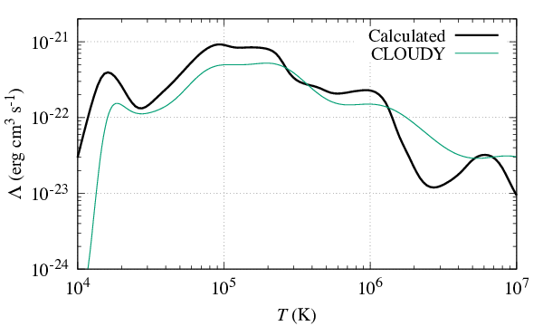
Figure 3 shows the calculated cooling function in the collisional ionization equilibrium (black line) that is consistent with the cooling function given by Cloudy (Ferland et al. 2017, green,). Since we omit the charge-exchange reaction, which works at K, the function is overestimated due to the survived H and lower ionized ions. Interestingly, our shows a depression at K compared with the function given by Cloudy, around which the gas can be thermally stable (). This may be due to the updated recombination rates of Fe. In this paper, we concentrate to study the nature of Galactic wind, deferring a further analysis on the depression for future work. In this article, we assume the collisional ionization equilibrium and use this cooling function.
Compton heating and photoionization heating are competitive processes against the radiative cooling in general. We neglect them for simplicity. In the case of the MW (irradiated by the metagalactic radiation field), they do not dominate over the cooling around the virial temperature unless (Gnat 2017, e.g.,). The outflow with a mass transfer rate of that is comparable to the star formation rate of the MW has a number density of . When the number density reaches at , the heating rate dominates over the cooling rate at with the solar metallicity and metagalactic radiation field at the current time (Gnat 2017). The cooling rate becomes comparable to that in the case of collisional ionization equilibrium (CIE) at K. At a higher temperature, the cooling rate is smaller than the CIE case by a factor of due to the photoionization yielding highly ionized ions. Note that, at a given electron temperature, an increment of in highly ionized ions reduces the line intensity because a potential energy of the bound electrons becomes large. Thus, the radiative heating is not expected to be important, and we neglect it for simplicity.
Heating due to the dissipation of the Alfvén waves can be comparable to the radiative cooling. Defining a scale height of the CR pressure as , we estimate the ratio of the radiative cooling rate to the heating rate due to the wave dissipation as
| (20) |
Since the transport of the CRs is determined by a combination of the advection and diffusion as described by Eq. (II), the characteristic length scale can be estimated as . Thus, the gas heating process may be mainly determined by the dissipation of Alfvén waves rather than the radiative process.
III wind equation and transonic point analysis
From the basic equations (5)-(II), we can derive the wind equation as
| (21) |
where the prime indicates the derivative with respect to (e.g., ), and we define
| (22) | |||
| (23) | |||
| (24) | |||
| (25) |
We assume for the smooth outflow solution. We will see that the role of CRs is important for this condition.
First, we review the primal properties of a steady flow in a gravitational potential. Considering the simplest case , , , and (i.e., analogous to a simple adiabatic solar wind solution) as an example, the sign of the wind equation depends on whether the flow is subsonic () or supersonic (). The subsonic flow with a negligible gravitational acceleration () shows always . This reflects simply the adiabatic expansion in vacuum. In contrast to this, a sufficiently large gravitational pull () corresponds to a negative numerator on the right-hand side of Eq. (21). Since the denominator is negative in the subsonic region, this results in . The accelerated flow passes the transonic point at which the conditions of should be satisfied so that is finite and positive. For a supersonic flow, the internal energy is no longer important for the fluid dynamics, and the condition of is . This means that the mean kinetic energy of particles in the fluid element is larger than the gravitational potential energy , i.e., the particles should be gravitationally unbound.
In our case, the CRs can accelerate the fluid by a term of , and can heat the fluid via the wave generation and dissipation (). The former makes the rate of adiabatic losses large, that is, too much CR pressure results in for a subsonic flow. On the other hand, for a supersonic flow, this additional pressure support helps to make . The latter acts in the opposite sense. The heating acts against the radiative or adiabatic cooling; thus a sufficient amount of CRs tends to make for a subsonic flow. For a supersonic flow, too much heating results in too high thermal pressure that dominates over the ram pressure of the fluid. In such a case, the condition of the smooth wind solution everywhere is not satisfied due to the existence of a pressure bump. These effects can be seen by rewriting the wind equation. Considering a subsonic flow as an example, from the condition of , we obtain
| (26) | |||||
Thus, when (), the CR pressure acts as the term of (the heating), and has an upper (lower) limit. For a supersonic flow, the inequality reverses. As we discussed in Sect. II, the plasma- has at the bottom region of the outflow. Thus, the Alfvén Mach number is about . Hence, the CRs contribute to realize the steady-state outflow via the term of , which acts as an additional pressure support for a supersonic flow. Note that the above argument appears because we adopt the steady-solution with everywhere.
Finally, we analyze the conditions of the transonic point following Breitschwerdt et al. 1991. 44 4 The original definition of by Breitschwerdt et al. 1991 includes the CR pressure by neglecting the CR diffusion. Recchia et al. 2016 considered the CR diffusion and also defined the with the CR pressure. In such definition, however, the expression of shows an apparent diverging point. To avoid this, we treat the CR pressure separately. Defining , we rewrite the wind equation as
| (27) |
where
| (28) |
At the transonic point , the conditions and should be satisfied simultaneously so that the velocity gradient is finite and positive. We obtain the gradient at by the linearization of the equation around the transonic point as
| (29) |
where and , respectively. Then, introducing the transformations of
we obtain
| (30) | |||
| (31) | |||
| (32) |
Substituting , we find the solution of this differential equation as
| (33) | |||
| (34) |
Since we consider the outflow solution (), we take the positive sign in front of the square root of . We show the expressions of and in the appendix.
To find the wind solution, we set the values (, , , , , , and ) at the transonic point as a boundary condition. The location of the transonic point is given by the condition of because contains the term of , which is a given function of . The velocity gradient at the transonic point is calculated by using Eq. (34), and then the gradients of other values (, , and ) are obtained. Integrating these differential equations from the transonic point toward the top and bottom boundaries, we can find a smooth solution with at arbitrary . Note that this method ensures the flow passing through the transonic point; however, it is not guaranteed whether the solution continues at the both boundaries with a positive and finite . For example, some boundary conditions lead to a flow showing at the subsonic region between the transonic point and bottom boundary that results in a divergence of the velocity gradient. Such behavior results from the effects of the radiative cooling, and the topology of the flow is different from the case of no radiative cooling (Breitschwerdt et al. 1991; Recchia et al. 2016, e.g.,). We can efficiently exclude such ‘failed’ solutions by starting from the transonic point.
IV Results
To derive the outflow solutions, we set boundary conditions at the transonic point . We fix two parameters as and (i.e., ). The subscript ‘tr’ indicates the values at the transonic point. We have chosen logarithmically spaced different values of other parameters for , and , that can be expressed by the following formula:
| (35) |
where symbolically indicates , , , and . The values of , , and are summarized in Table 2.
| cm-3 | K | eV cm-3 | kpc | |
| cm-3 | K | eV cm-3 | kpc | |
Note that . Then, we integrate the Eqs. (5)-(II) from the transonic point toward the bottom boundary and toward the top boundary by the fourth Runge-Kutta method, respectively. For those boundary conditions, successful outflow solutions we consider satisfy that , , and at , and at , and at , where the subscripts ‘bt’ and ‘tp’ denote the values at the bottom boundary and top boundary, respectively. We apply this procedure for 10 horizontal positions, kpc, and find solutions in total as a result.


We discuss the nature of the outflow using the solution at kpc for , , , and as a representative result. Note that . The values at the bottom boundary of this solution are , , , , and , respectively. The top panel of Fig. 4 shows the velocities of (solid line), (dots), and (dashed line). Note that . The transonic point is located at kpc. becomes negative at kpc because in Equation (24), the term of dominates over the gravitational acceleration (i.e., ). rapidly decreases from kpc due to the radiative cooling. The minimum temperature is about K at which . Then, the cooling is balanced by the heating due to the wave dissipation. Since the cooling rate decreases with increasing the velocity and area cross section of the flux tube (), the outflow is slightly heated due to the wave dissipation. The outflow begins to be adiabatically cooled again from kpc because the CR pressure drops exponentially. This exponential decay of results from the effects of the CR diffusion. Note that, if we consider a case of no diffusion of CRs (), the CR transport equation (II) could be rewritten as (Breitschwerdt et al. 1991, e.g.,). The bottom panel of Fig. 4 shows the pressures of (solid line), (dots), and (dashed line). The CR pressure is well represented by for this solution.

We consider the effects of the amount of CRs. Figure 5 shows three solutions at kpc for (blue), (green), and (red). The other parameters are the same as in Fig. 4. Table 3 summarizes the values at the bottom boundary for these three solutions.
| K | ||||
|---|---|---|---|---|
| 0.316 | 5.23 | 4.70 | 2.12 | 0.456 |
| 0.750 | 4.85 | 4.30 | 1.80 | 1.04 |
| 2.37 | 3.46 | 3.25 | 0.969 | 2.90 |
As shown in Table 3, the thermal pressure is anticorrelated to the CR pressure . Since the acceleration by large pressures overwhelming the gravitational acceleration at the subsonic region makes (see Section III), the total pressure may be regulated to a certain degree to satisfy the given boundary conditions at the transonic point. Note that the thermal pressures at the transonic points are the same as each of the three solutions (i.e. the total pressures are different); therefore, the regulation of the total pressure at the bottom boundary is not so obvious. Figure 6 shows the total pressure (top panel) and ratio of the pressures (bottom panel) for these three solutions.


In the case of the relatively small CR pressure (blue line), a relatively large thermal pressure is required. Since the temperature should be around the virial temperature, this requirement results in a relatively large density. Then, the outflow suffers the radiative cooling at a rate of , and the CR pressure becomes the dominant component to accelerate the outflow. Contrary to this, when the CR pressure is relatively large (red line), the required thermal pressure becomes low, which results in a relatively small density. Since the cooling rate depends on and the heating rate depends on , the temperature (and thermal pressure) remains to be high. Thus, a smaller (larger) CR pressure results in a slower and colder (faster and hotter) outflow. Note that the amount of CRs at a local point is also determined by the diffusion coefficient. Figure 7 shows the spatial profile of the coefficient . The hotter wind results from a larger because the CRs can reach at a higher .


Here, we confirm the above discussion from the overall trend of the solutions. Figure 8 shows the values at the bottom and top boundaries for the derived solutions at kpc. The top panel shows the relation between , , and . The total pressure range is . The mass flux shows a roughly linear dependence on the total pressure. As shown in Figure 9, this mainly results from the dependence of , while does not depend on the total pressure (a scattering of is about a factor of 2). Since the temperature should be around the virial temperature (indeed our solutions show K), this dependence simply reflects the equation of state . Then, a faster outflow at the subsonic region can reach a larger height, at which the gravitational acceleration is negligible compared with the rate of the adiabatic cooling, so it tends to make . Thus, the larger pressure results in a more massive outflow with fixed velocity rather than accelerating the outflow with fixed mass. The bottom panel of Fig. 8 shows the relation between , , and . As we discussed above, a relatively small (large) CR pressure results in a cold (hot) outflow. Thus, the mass flux is determined by the total pressure, while the properties of the outflow (especially the temperature) are controlled by the amount of CRs.
We discuss the fate of the outflow in the three cases summarized in Table 3.


Figure 10 shows the ratio of the cooling rate to the heating rate (top panel) and the cooling time (bottom panel). Since the heating due to the wave dissipation ceases with the exponential decrement in the CR pressure, the gas eventually cools. Considering the solution with (blue) as an example, the cooling time is shorter than Gyr. Such cooled gas eventually decelerates due to the gravitational pull, that is, we cannot regard that the solution continues to infinity. It may be difficult to think that such solution represents a stable and steady-state solution, rather the solution may be related to phenomena for which the gas falls back to the Galactic disk. In the following, we denote the solutions with Gyr and at the top boundary as ‘fall back’ solutions. Note that, since the number density becomes smaller than at kpc, the radiative heating rate can dominate over the cooling rate at K (see section II.3). The wind could be isothermal with , and the isothermal temperature increases (decreases) with decreasing (increasing) the number density. Thus, if the ‘fall back’ phenomena are related to a condensation of gas, the radiative heating may not affect the expectation of the ‘fall back’ phenomena. Condensation and precipitation are indeed likely processes of a thermally unstable gas.
Finally, we estimate the total mass carried by the outflow per unit time as
| (36) | |||
| (37) | |||
| (38) |
where denotes the horizontal location as . The carried mass per unit time at a radius of is , which is estimated from the mass flux integrated along the axial symmetric ring at the with a width of . The factor of 2 indicates the two directions of the outflow, and . The total carried mass per unit time is . Since we suppose the axial symmetry, this estimation may give an upper limit of the mass carried by the outflow. Note that and were defined in a way similar to previous studies (Breitschwerdt et al. 1991, e.g.,). Since we have many possible sets of solutions, we derive a statistical average.


Figure 11 shows the average of as a function of the CR pressure at the bottom boundary. The green boxes indicate the average for all the solutions. As we discussed above, the mass transfer rate does not depends sensitively on the CR pressure; it depends on the thermal pressure (see also Fig. 8). The % solutions are the ‘fall back’ solutions. The ‘fall back’ outflow tends to be massive because an efficient radiative cooling is required.

Figure 12 shows the averaged number density and temperature at the bottom boundary for the CR pressure of . The average of number density for the ‘fall back’ solutions is roughly 2 times thath for all the solutions. This is also indicated by the mass transfer rate. The temperature is around the virial temperature in both cases. The boundary conditions are consistent with the X-ray observations (Nakashima et al. 2018, e.g.,) and numerical simulation (Girichidis et al. 2018); therefore the ‘fall back’ solutions are expected to be realized.
V Summary and Discussion
We have solved the steady state-Galactic wind including the effects of the radiative cooling, CR diffusion, and heating due to the dissipation of Alfvén waves that are excited by the CRs. We have found 327,254 solutions in total. For the dynamics of the thermal gas, the CR pressure acts as the term of or heating depending on the Alfvén Mach number. The former is dominant for , while the latter is dominant for . The mass flux of the outflow mainly depends on the thermal pressure. The CR pressure determines the cooling and heating balance. When the CR pressure is smaller than the thermal pressure, the outflow tends to have a lower temperature at the vertical height of kpc. A fraction of the solutions have a short cooling time of Gyr with the cooling rate larger than the heating rate at the top boundary kpc. For these solutions, is required. We have regarded that such an outflow finally falls back to the Galactic disk. The total mass carried by the outflow per unit time has been estimated as . Thus, in terms of the mass budget, the Galactic star formation history is controlled by whether the outflow falls back to the Galactic disk or not, which is determined by the ratio of the thermal pressure to the CR pressure.
Here we discuss about the boundary conditions at the kpc for the ‘fall back’ solutions using K, , , and kpc as an example (see Table 3). The temperature comparable with the virial temperature for a distance of kpc may be required to drive the wind, and it is consistent with the X-ray observations (Nakashima et al. 2018, e.g.,). A number density of may be nontrivial, though it is supported by numerical simulations (Girichidis et al. 2018, e.g.,). If the hot, tenuous gas above the Galactic disk secularly exists due to the balance of energy injection by supernovae and radiative loss, , where and are the energy injection rate of supernovae and conversion efficiency, respectively, we obtain
| (39) | |||||
The energy injection rate of the supernovae, , corresponds to an event rate of three times per hundred years. It is expected that roughly a tenth of the kinetic energy of a supernova is converted to the turbulence in the ISM. Thus, a conversion efficiency of means that roughly a tenth of the energy of the ISM turbulence is consumed to form the hot, tenuous gas. The wind may have a velocity comparable to the virial velocity, , which is consistent with our model calculation. The total mass carried by the wind per unit time can be estimated as
| (40) | |||||
Note that the CR pressure is required to transfer the metals at a height of kpc by the wind. When the CR pressure satisfies , the wind suffers the significant radiative cooling. In this case, the solution cannot be extended to infinity. This might be related to the possible existence of ‘fall back’ phenomena, which are interesting as a gas replenishment mechanisms. Thus, to realize a steady Galactic system, the condition of
| (41) | |||||
may be required. Since the wind carries the CRs, we can estimate an injection power of CRs in the Galactic disk as
| (42) | |||||
Thus, if the CRs are injected by the supernovae, the wind suffers the significant radiative cooling. This system can be stable for variations of the star formation rate. Let us suppose that the star formation rate increases from the current average rate of a few . Then, the CR pressure becomes larger than the thermal pressure due to an increment in the star formation rate (i.e., increment in the event rate of the supernovae), and the wind can reach at a height of kpc without the significant radiative cooling. Thus, the Galactic disk secularly loses the gaseous matter, leading to a decrement in the star formation rate. In contrast, with decreasing the CR pressure, the radiative cooling of wind becomes significant, which may lead to the ‘fall back’ phenomena and an increment in the star formation rate. This self-regulation effect by the wind possibly explains the constant star formation rate averaged by a time scale of Gyr (Haywood et al. 2016, e.g.,). Hence, it is important to study the conversion efficiency and existence of the ‘fall back’ phenomena, which are not analyzed in this article. We will address them in our future work.
We compare our model with current observations of MW’s CGM. Miller & Bregman 2015 analyzed emission line measurements of O VIII and O VII from XMM-Newton/EPIC-MOS spectra, and gave some constraints for the hot CGM assuming a one-dimensional density structure,
| (43) |
where is the galactocentric radius. From the O VIII observations, the parameters , and were derived as and , where we omit to display the error, and the range of parameter values results from optical depth corrections. These constraints are mainly derived from the O VIII measurements. They estimated the total mass of the X-ray emitting gas as for kpc and for kpc.55 5 The analyzed hot X-ray emitting medium was referred as ‘hot halo’ but the derived length scale is comparable with the CGM we supposed. Therefore, we refer to the ‘hot halo’ of Miller & Bregman 2015 as ‘CGM’ in this article. In their analysis, the CGM was assumed to have a constant temperature profile in CIE with fixed and a metallicity of . Although these constraints are based on a different situation from our wind, the total mass of our wind should has been comparable to the estimated mass given by the intensity of the emission lines (almost equivalent to the column density). The effects of the lower metallicity () are discussed later. The order of magnitude estimate of the total mass may be written as
| (44) | |||||
If ‘fall back’ phenomena really occur over the cooling time of , the expected mass inflow rate () onto the disk might be sufficiently large in replenishing the gas of the Galactic disk. From our model calculations, we estimate the statistical average of the total mass as
| (45) | |||||
| (46) | |||||
| (47) |
Then, we obtain for all solutions and for the ‘fall back’ solutions. Note that, in our scenario, the observationally constrained mass should include other components, such as metal-polluted intergalactic medium (IGM) heated by the wind termination shock. In addition, the mass of the inflow from the CGM to the Galactic disk (i.e., the total mass of the CGM) should be larger than the mass carried by the wind because a comparable mass is consumed for the star formation. Thus, the total mass of the wind estimated by our model can still be consistent with the constraints given by Miller & Bregman 2015 in terms of the mass budget that may explain the observed star formation history.
Miller & Bregman 2015 also obtained the subsolar metallicity of the hot CGM by combinations of the emission (O VIII) and absorption (O VII) analysis and the pulsar’s dispersion measure toward the Large Magellanic Cloud. Since the lower metallicities reduce the radiative cooling rate, it might be interesting to investigate how the wind profile may change from our calculations with .


The top panel of Figure 13 shows the wind solutions with the same boundary conditions as the case of Figure 5 but the radiative cooling rate is reduced by a factor of 0.1. The reduced cooling rate obviously results in a hotter wind; however, the other profiles of , and are not so changed. The heating rate due to the CRs is still smaller than the reduced cooling rate at a lower . Once the wind passes the transonic point, the thermal pressure becomes less important and the wind is mainly driven by the CR pressure. Thus, for the typical conditions of the MW we discussed above, the down to does not change our expectations. This is confirmed by the overall trend of the solutions with the reduced cooling function (the bottom panel of Figure 13). The result is similar to the case of (Figure 8). Note that the number of solutions with a reduced cooling rate is 580,014 (127,633 for the ‘fall back’ solutions). Thus, if we compare the same boundary conditions, the reduced cooling rate results in launching the wind ‘more easily’ than the case of the solar metallicity. The average total masses are for all solutions and for the ‘fall back’ solutions. From such insensitive metallicity dependence, we may regard that our picture of a quasi-steady-star formation in the MW has been continued from Gyr ago when the amount of metals was smaller than the current one.
Comparison of the current CR energy density at the Galactic disk with our estimates may be important. Cerri et al. 2017 studied the CR propagation in the Galactic disk below a height of kpc to explain the spatial variation of -ray spectral slope observed by Fermi LAT collaboration (Acero et al. 2016). To derive the CR energy density (or pressure) from the -ray observations, we must know the conditions of the thermal gas including all the components (diffuse hot medium, H I cloud, molecular cloud, etc.) in detail because the -ray photons result from the hadronic interaction between the CR protons and thermal protons (). However, the conditions of the thermal gas are not fully understood. Moreover, the propagation of CRs around the molecular cloud is also an unsettled issue in terms of the effects of the magnetic mirror with a local turbulent field (Lazarian & Xu 2021, e.g.,). Thus, it would be better to discuss the both of the observational estimate and theoretical prediction rather than the observation only. The propagation model of Cerri et al. 2017 is based on an anisotropic diffusion coefficient tensor given by pitch-angle scattering; the diffusion along the guide magnetic field is stronger than the perpendicular one. The global configuration of the magnetic field controls the spatial distribution of the CR spectral slope and energy density and is assumed to have a substantial poloidal component. This situation is similar to our model. Their model does not include the various thermal gas conditions, and the calculated energy density and spectral slope of the CR protons are directly compared to the estimated values from the observations. This procedure corresponds to CRs that are approximated to propagate in a diffuse medium with a uniform density structure. The resultant CR energy density of (equivalently, ) can be consistent with the Fermi LAT observations at kpc.66 6 The observations and models provide the number density of CR protons with an energy of GeV to be . We estimate the energy density as . This estimate may be valid because the spectral slope of CRs is estimated as (almost all energy is deposited by CRs with an energy of GeV). At kpc, the predicted energy density depleting toward the Galactic center is significantly lower than that estimated from the observations (). These estimates satisfy the inequality we discussed above. Note that the CR pressure of is sufficiently large in launching the wind depending on the thermal gas conditions. Thus, the current state of the MW implies that the cold wind is driven, eventually falling back to the disk in the future.
Observations of external galaxies show that the CGM consists of not only highly ionized species like O VI but also lower-ionized species like H I, C II, Mg II, and so on (Tumlinson et al. 2017, and references therein). The absorption lines of these lower-ionized species are also observed at a distance of kpc from the host galaxy. Our solutions imply that the outflow can transfer such lower-ionized species to a height of kpc if the radiative cooling is efficient. The condition for efficient radiative cooling is . Note that the ionization state is affected by photoionization which is omitted in this paper. Thus, we have to pay attention whether the O VI absorption line really indicates the existence of hot gas (Breitschwerdt & Schmutzler 1999, see). On the other hand, photoionization reduces the number of lower-ionized species. Thus, the existence of the lower ionized species indicates that the temperature of gas is low or the condensation of gas occurs to shield itself from the photoionizing photons. In any case, an efficient cooling process is required. We will study the ionization state and condensation of gas at a height of kpc in future work.
We have assumed that the outflow travels along the vertical direction so that the required energy is approximately minimum. This condition, however, is strictly given by . Thus, the outflow may have at least two-dimensional spatial structure, like a biconical structure, in reality. It is reported by numerical simulation that the CR pressure can affect the spatial structure of wind (Hopkins et al. 2018). The far-ultraviolet observation of NGC 3079 implies an X-shape wind (Hodges-Kluck et al. 2020). Thus, it would be worth to investigating the relation between the wind condition and its morphology. The wind morphology may depend on how the diffusion coefficient is assumed. The multidimensional diffusion coefficient (i.e., diffusion tensor) is also actively discussed issue in the CR transport literature (e.g., Cerri et al. 2017, , and references therein). Zirakashvili et al. 1996 studied an axially symmetric wind considering the Galactic disk rotation and introduced an effective CR adiabatic index as a possibly useful method,
| (48) |
so that the CR pressure can be expressed as . It may simplify the analysis of the transonic ‘surface’ of the multidimenstional wind and the systematic parameter study of the diffusion coefficient. We hope to extend our model to a multidimensional one in our future work.
| (49) | |||
and
| (50) |
References
- Acero et al. (2016) Acero, F., Ackermann, M., Ajello, M., et al. 2016, ApJS, 223, 26, doi: 10.3847/0067-0049/223/2/26
- Achterberg (1981a) Achterberg, A. 1981a, A&A, 98, 195
- Achterberg (1981b) —. 1981b, A&A, 98, 161
- Altun et al. (2007) Altun, Z., Yumak, A., Yavuz, I., et al. 2007, A&A, 474, 1051, doi: 10.1051/0004-6361:20078238
- Arnaud & Rothenflug (1985) Arnaud, M., & Rothenflug, R. 1985, A&AS, 60, 425
- Asplund et al. (2009) Asplund, M., Grevesse, N., Sauval, A. J., & Scott, P. 2009, ARA&A, 47, 481, doi: 10.1146/annurev.astro.46.060407.145222
- Boulares & Cox (1990) Boulares, A., & Cox, D. P. 1990, ApJ, 365, 544, doi: 10.1086/169509
- Bregman & Lloyd-Davies (2007) Bregman, J. N., & Lloyd-Davies, E. J. 2007, ApJ, 669, 990, doi: 10.1086/521321
- Breitschwerdt et al. (1991) Breitschwerdt, D., McKenzie, J. F., & Voelk, H. J. 1991, A&A, 245, 79
- Breitschwerdt & Schmutzler (1999) Breitschwerdt, D., & Schmutzler, T. 1999, A&A, 347, 650. https://arxiv.org/abs/astro-ph/9902268
- Cerri et al. (2017) Cerri, S. S., Gaggero, D., Vittino, A., Evoli, C., & Grasso, D. 2017, J. Cosmology Astropart. Phys, 2017, 019, doi: 10.1088/1475-7516/2017/10/019
- Ferland et al. (2017) Ferland, G. J., Chatzikos, M., Guzmán, F., et al. 2017, Rev. Mexicana Astron. Astrofis., 53, 385. https://arxiv.org/abs/1705.10877
- Ferrière (2001) Ferrière, K. M. 2001, Reviews of Modern Physics, 73, 1031, doi: 10.1103/RevModPhys.73.1031
- Gabici et al. (2019) Gabici, S., Evoli, C., Gaggero, D., et al. 2019, International Journal of Modern Physics D, 28, 1930022, doi: 10.1142/S0218271819300222
- Ginzburg & Syrovatskii (1964) Ginzburg, V. L., & Syrovatskii, S. I. 1964, The Origin of Cosmic Rays
- Girichidis et al. (2018) Girichidis, P., Naab, T., Hanasz, M., & Walch, S. 2018, MNRAS, 479, 3042, doi: 10.1093/mnras/sty1653
- Gnat (2017) Gnat, O. 2017, ApJS, 228, 11, doi: 10.3847/1538-4365/228/2/11
- Gronenschild & Mewe (1978) Gronenschild, E. H. B. M., & Mewe, R. 1978, A&AS, 32, 283
- Hahn et al. (2014) Hahn, M., Badnell, N. R., Grieser, M., et al. 2014, ApJ, 788, 46, doi: 10.1088/0004-637X/788/1/46
- Hayakawa et al. (1958) Hayakawa, S., Ito, K., & Terashima, Y. 1958, Progress of Theoretical Physics Supplement, 6, 1, doi: 10.1143/PTPS.6.1
- Haywood et al. (2016) Haywood, M., Lehnert, M. D., Di Matteo, P., et al. 2016, A&A, 589, A66, doi: 10.1051/0004-6361/201527567
- Hodges-Kluck et al. (2020) Hodges-Kluck, E. J., Yukita, M., Tanner, R., et al. 2020, ApJ, 903, 35, doi: 10.3847/1538-4357/abb884
- Hopkins et al. (2018) Hopkins, P. F., Wetzel, A., Kereš, D., et al. 2018, MNRAS, 480, 800, doi: 10.1093/mnras/sty1690
- Inutsuka et al. (2015) Inutsuka, S. i., Inoue, T., Iwasaki, K., et al. 2015, in Astronomical Society of the Pacific Conference Series, Vol. 498, Numerical Modeling of Space Plasma Flows ASTRONUM-2014, ed. N. V. Pogorelov, E. Audit, & G. P. Zank, 75
- Ipavich (1975) Ipavich, F. M. 1975, ApJ, 196, 107, doi: 10.1086/153397
- Janev & Smith (1993) Janev, R. K., & Smith, J. J. 1993, Cross Sections for Collision Processes of Hydrogen Atoms with Electrons, Protons and Multiply Charged Ions, 192
- Jokipii (1966) Jokipii, J. R. 1966, ApJ, 146, 480, doi: 10.1086/148912
- Kennicutt & Evans (2012) Kennicutt, R. C., & Evans, N. J. 2012, ARA&A, 50, 531, doi: 10.1146/annurev-astro-081811-125610
- Kotelnikov & Milstein (2019) Kotelnikov, I. A., & Milstein, A. I. 2019, Phys. Scr, 94, 055403, doi: 10.1088/1402-4896/ab060a
- Kulsrud & Pearce (1969) Kulsrud, R., & Pearce, W. P. 1969, ApJ, 156, 445, doi: 10.1086/149981
- Kulsrud (2005) Kulsrud, R. M. 2005, Plasma physics for astrophysics
- Lazarian & Xu (2021) Lazarian, A., & Xu, S. 2021, arXiv e-prints, arXiv:2106.08362. https://arxiv.org/abs/2106.08362
- Lee & Völk (1973) Lee, M. A., & Völk, H. J. 1973, Ap&SS, 24, 31, doi: 10.1007/BF00648673
- Lennon et al. (1988) Lennon, M. A., Bell, K. L., Gilbody, H. B., et al. 1988, Journal of Physical and Chemical Reference Data, 17, 1285, doi: 10.1063/1.555809
- Lerche (1966) Lerche, I. 1966, Physics of Fluids, 9, 1073, doi: 10.1063/1.1761804
- Lerche (1967) —. 1967, ApJ, 147, 689, doi: 10.1086/149045
- Lestinsky et al. (2009) Lestinsky, M., Badnell, N. R., Bernhardt, D., et al. 2009, ApJ, 698, 648, doi: 10.1088/0004-637X/698/1/648
- Lockman (1984) Lockman, F. J. 1984, ApJ, 283, 90, doi: 10.1086/162277
- McKee & Ostriker (1977) McKee, C. F., & Ostriker, J. P. 1977, ApJ, 218, 148, doi: 10.1086/155667
- Mewe (1972) Mewe, R. 1972, A&A, 20, 215
- Mewe et al. (1986) Mewe, R., Lemen, J. R., & van den Oord, G. H. J. 1986, A&AS, 65, 511
- Mewe et al. (1980a) Mewe, R., Schrijver, J., & Sylwester, J. 1980a, A&AS, 40, 323
- Mewe et al. (1980b) —. 1980b, A&A, 87, 55
- Miller & Bregman (2015) Miller, M. J., & Bregman, J. N. 2015, ApJ, 800, 14, doi: 10.1088/0004-637X/800/1/14
- Mitnik & Badnell (2004) Mitnik, D. M., & Badnell, N. R. 2004, A&A, 425, 1153, doi: 10.1051/0004-6361:20041297
- Miyamoto & Nagai (1975) Miyamoto, M., & Nagai, R. 1975, PASJ, 27, 533
- Murakami et al. (2006) Murakami, I., Kato, T., Kato, D., et al. 2006, Journal of Physics B Atomic Molecular Physics, 39, 2917, doi: 10.1088/0953-4075/39/14/001
- Nahar (1995) Nahar, S. N. 1995, ApJS, 101, 423, doi: 10.1086/192248
- Nahar (1998) —. 1998, Phys. Rev. A, 58, 3766, doi: 10.1103/PhysRevA.58.3766
- Nahar (2000) —. 2000, ApJS, 126, 537, doi: 10.1086/313307
- Nahar (2006) —. 2006, ApJS, 164, 280, doi: 10.1086/501503
- Nahar & Pradhan (1997) Nahar, S. N., & Pradhan, A. K. 1997, ApJS, 111, 339, doi: 10.1086/313013
- Nahar & Pradhan (1999) —. 1999, A&AS, 135, 347, doi: 10.1051/aas:1999447
- Nahar et al. (2001) Nahar, S. N., Pradhan, A. K., & Zhang, H. L. 2001, ApJS, 133, 255, doi: 10.1086/319187
- Nakashima et al. (2018) Nakashima, S., Inoue, Y., Yamasaki, N., et al. 2018, ApJ, 862, 34, doi: 10.3847/1538-4357/aacceb
- Navarro et al. (1996) Navarro, J. F., Frenk, C. S., & White, S. D. M. 1996, ApJ, 462, 563, doi: 10.1086/177173
- Novotný et al. (2012) Novotný, O., Badnell, N. R., Bernhardt, D., et al. 2012, ApJ, 753, 57, doi: 10.1088/0004-637X/753/1/57
- Osterbrock & Ferland (2006) Osterbrock, D. E., & Ferland, G. J. 2006, Astrophysics of gaseous nebulae and active galactic nuclei
- Recchia et al. (2016) Recchia, S., Blasi, P., & Morlino, G. 2016, MNRAS, 462, L88, doi: 10.1093/mnrasl/slw136
- Savin et al. (2002) Savin, D. W., Behar, E., Kahn, S. M., et al. 2002, ApJS, 138, 337, doi: 10.1086/323388
- Shapiro & Field (1976) Shapiro, P. R., & Field, G. B. 1976, ApJ, 205, 762, doi: 10.1086/154332
- Sofue (2012) Sofue, Y. 2012, PASJ, 64, 75, doi: 10.1093/pasj/64.4.75
- Tumlinson et al. (2017) Tumlinson, J., Peeples, M. S., & Werk, J. K. 2017, ARA&A, 55, 389, doi: 10.1146/annurev-astro-091916-055240
- Volk & McKenzie (1981) Volk, H. J., & McKenzie, J. F. 1981, in International Cosmic Ray Conference, Vol. 9, International Cosmic Ray Conference, 246–249
- Wentzel (1968) Wentzel, D. G. 1968, ApJ, 152, 987, doi: 10.1086/149611
- Zatsarinny et al. (2006) Zatsarinny, O., Gorczyca, T. W., Fu, J., et al. 2006, A&A, 447, 379, doi: 10.1051/0004-6361:20053737
- Zatsarinny et al. (2003) Zatsarinny, O., Gorczyca, T. W., Korista, K. T., Badnell, N. R., & Savin, D. W. 2003, A&A, 412, 587, doi: 10.1051/0004-6361:20031462
- Zatsarinny et al. (2004) —. 2004, A&A, 417, 1173, doi: 10.1051/0004-6361:20034174
- Zirakashvili et al. (1996) Zirakashvili, V. N., Breitschwerdt, D., Ptuskin, V. S., & Voelk, H. J. 1996, A&A, 311, 113