DualFormer: Local-Global Stratified Transformer for Efficient Video Recognition

Yuxuan Liang Affiliation: Sea AI Lab National University of Singapore Pan Zhou Roger Zimmermann Affiliation: Sea AI Lab National University of Singapore Shuicheng Yan E-mail {yuxliang,rogerz}@comp.nus.edu.sg {zhoupan,ysc}@sea.com Affiliation:

Abstract

While transformers have shown great potential on video recognition with their strong capability of capturing long-range dependencies, they often suffer high computational costs induced by the self-attention to the huge number of 3D tokens. In this paper, we present a new transformer architecture termed DualFormer, which can efficiently perform space-time attention for video recognition. Concretely, DualFormer stratifies the full space-time attention into dual cascaded levels, i.e., to first learn fine-grained local interactions among nearby 3D tokens, and then to capture coarse-grained global dependencies between the query token and global pyramid contexts. Different from existing methods that apply space-time factorization or restrict attention computations within local windows for improving efficiency, our local-global stratification strategy can well capture both short- and long-range spatiotemporal dependencies, and meanwhile greatly reduces the number of keys and values in attention computation to boost efficiency. Experimental results verify the superiority of DualFormer on five video benchmarks against existing methods. In particular, DualFormer achieves 82.9%/85.2% top-1 accuracy on Kinetics-400/600 with $\sim$ 1000G inference FLOPs which is at least 3.2 $\times$ fewer than existing methods with similar performance. We have released the source code at https://github.com/sail-sg/dualformer.

Keywords:

efficient video transformer, local and global attention.

1 Introduction

Video recognition is a fundamental task in computer vision, such as action recognition [5] and event detection [18]. Like in image-based tasks [27, 44, 17], Convolutional Neural Networks (CNNs) are often taken as backbones for video recognition models [32, 48, 50, 5, 12, 13]. Though successful, it is challenging for convolutional architectures to capture long-range spatiotemporal dependencies across video frames due to their limited receptive field.

Recently, transformers [51] have become an alternative paradigm for visual modeling beyond CNNs, demonstrating great potential in a series of image processing tasks [54, 34, 42, 55, 52, 62]. A pioneering work is the Vision Transformer (ViT) [10] which replaces the inherent inductive bias of locality in convolutions by global relation modeling with multi-head self-attention (MSA) [51]. Soon the vision community extends the application of MSA from static images to videos considering its remarkable power for capturing long-range spatiotemporal dependencies [38, 11, 3, 1]. Concretely, a video is first partitioned into non-overlapping 3D patches, similar as in NLP tasks [51], which then serve as input tokens for transformers to jointly learn short- and long-range relations within a video.

Refer to caption — Figure 1: Accuracy vs. FLOPs on Kinetics [25]. Ours-B is the base version of DualFormer.

One of the major challenges for applying transformers to video data is their low efficiency. Due to the MSA operation, the computational cost of video transformers grows quadratically with the increasing number of tokens, and may even become totally unaffordable for some high spatial resolution or long videos. To alleviate this issue, TimeSformer [3] and ViViT [1] factorize the full space-time self-attention along temporal and spatial dimensions separately to achieve a balance between accuracy and efficiency in video recognition. Inspired by the observation that near tokens are usually more related than distant ones [46], Video Swin Transformer [35] applies the inductive bias of locality at each transformer layer via performing self-attention in the non-overlapping local windows. Though effective, both the space-time factorization and the local-window based attention scheme contradict the aim of applying full space-time attention, i.e., to jointly capture local and global spatiotemporal dependencies within one layer, and thus impair the performance of video transformers.

In this work, we present a new video transformer architecture entitled DualFormer for efficient video recognition. DualFormer stratifies the full space-time attention into dual cascaded levels: 1) Local-Window based Multi-head Self-Attention (LW-MSA) to extract short-range interactions among nearby tokens; and 2) Global-Pyramid based MSA (GP-MSA) to capture long-range dependencies between the query token and the coarse-grained global pyramid contexts. In this manner, DualFormer significantly reduces the number of keys and values in attention computation, and achieves much higher efficiency over existing video transformers [3, 1, 35] with comparable performance, as shown in Figure 1.

Figure 2 shows how a query patch (in red) attends to its surroundings in a DualFormer block. Following the intuition that tokens closer to each other are more likely to be correlated [34, 59], we first perform LW-MSA at a fine-grained level to allow each patch to interact with its neighbors within a local window. This strategy has also been verified to be efficient and memory-friendly by recent studies [34, 59, 8, 35, 6]. Next, at the global level, a query patch attends to the full region of interest at a coarse granularity via GP-MSA. To be specific, we first extract global contextual priors with different pyramid scales for multi-scale scene interpretation (see the two scales, i.e. small windows and large windows, in Figure 2(d)). These global priors then pass global contextual information to the query tokens via MSA. Since such priors are extracted at a coarse-grained level, their number is much smaller than the original token number, leading to far less computation cost in capturing global information than the full space-time attention. In contrast to the space-time factorization in TimeSformer [3] and ViViT [1] and the locality-based scheme in Swin [35], this dual-level attention design not only enables our model to have the global receptive field at each block, but is also efficient in attention computations.

Extensive experimental results on five video benchmarks validate the superiority of our DualFormer in terms of accuracy and FLOPs. In particular, our DualFormer achieves 82.9%/85.2% top-1 accuracy on Kinetics-400/600 [25] with only $\sim$ 1000 GFLOPs which is 3.2 $\times$ and 16.2 $\times$ fewer than the previous state-of-the-art methods, i.e., Swin [34] and ViViT [1], respectively. We strongly believe that such gains on efficiency benefit real-world deployments of video recognition models, especially for deployments on edge devices. See detailed comparison on Kinetics-400/600 in Figure 1. Furthermore, our model also achieves state-of-the-art performance on three smaller datasets under transfer learning settings.

2 Related Work

CNNs for Video Recognition. CNN-based video recognition models can be categorized into two groups: 2D CNNs and 3D CNNs [31]. For the first group [24, 53], each video frame is processed separately by 2D convolutions and then aggregated along the time axis at the top of the network. However, some studies point out that 2D convolutions cannot well capture the information along the temporal dimension [32, 37, 36, 22]. The second group learns spatiotemporal video representation via 3D convolutions by aggregating space-time features and are difficult to optimize [21, 48, 58, 16, 15]. Thus, the current trend for 3D CNN-based video recognition is to boost efficiency. For example, I3D [5] expands pretrained 2D CNNs [27, 44, 17] into 3D CNNs; some recent works [41, 57, 50, 49, 13, 12] factorize 3D convolutions into spatial and temporal filters, demonstrating even higher accuracy than vanilla 3D CNNs. Unfortunately, most of the 2D and 3D CNNs cannot capture long-range spatiotemporal dependencies due to their limited receptive fields, which leads to sub-optimal recognition performance.

Transformers for Video Recognition. Recently, transformers are applied to model spatiotemporal dependencies for video recognition [38, 11, 3, 4, 1, 61, 35, 39] by virtue of their great power in capturing long-range dependencies [10, 47, 34, 8]. With pretraining on a large-scale image dataset, video transformers achieve promising performance on video benchmarks [3, 1, 35], such as Kinetics-400/600. However, the potential of video transformers is significantly limited by the considerable computational complexity of performing full space-time attention. Various approaches have been proposed to reduce such computation cost [3, 4, 1, 61, 35]. For instance, TimeSformer [3] factorizes the full space-time attention into spatial and temporal dimensions. Similarly, ViViT [1] examines three variants of space-time factorization for computation reduction. X-ViT [4] approximates the space-time attention by restricting the temporal attention to a local temporal window and using a mixing strategy. Video Swin Transformer [35] introduces an inductive bias of locality to transformers for video understanding. However, these attempts focus on either space-time factorization or restricting attention computation locally, crippling the capability of MSA in capturing long-range dependencies. To solve this, we present a new transformer called DualFormer to improve the efficiency of video transformers, by alternatively capturing fine-grained local interactions and coarse-grained global information within each block. Besides, there are some concurrent works enhancing transformers [60, 29] or exploring self-supervised pretraining schemes [40, 56] for video recognition.

3 Methodology

We start by summarizing the overall architecture of DualFormer in Sec. 3.1, and then elaborate on its basic block in Sec. 3.2 by well introducing the two types of attention, including Local-Window based Multi-head Self-Attention (LW-MSA) and Global-Pyramid based MSA (GP-MSA). Afterward, we explain the network configuration for constructing our DualFormer in Sec. 3.3. Finally, we discuss the differences between our DualFormer and related works in Sec. 3.4.

3.1 Overall Architecture

Figure 3 shows the overall architecture of the proposed DualFormer. It takes a video clip $\mathcal{X}\in\mathbb{R}^{T\times H\times W\times 3}$ as input, where $T$ stands for the number of frames and each frame consists of $H\times W\times 3$ pixels. To accommodate high-resolution video-based tasks, our model leverages a hierarchical design [11, 59, 34, 35] to produce decreasing-resolution feature maps from early to late stages. First, we partition a video clip into non-overlapping 3D patches of size $2\times 4\times 4\times 3$ and employ a linear layer for projection, resulting in $\frac{T}{2}\times\frac{H}{4}\times\frac{W}{4}$ visual tokens with feature channel dimension $C$ . Then, as shown in Figure 3, these tokens go through the four stages of DualFormer for learning visual representations. At each stage $s\in\{1,2,3,4\}$ , we sequentially stack $N_{s}$ DualFormer blocks for spatiotemporal learning, where $N_{s}$ controls the capacity of each model stage. Each DualFormer block consists of dual cascaded levels of self-attention mechanisms: LW-MSA for learning short-range interactions within local windows, and GP-MSA for capturing long-range context information within the whole video. Additionally, a convolution-based Position Encoding Generator (PEG) [9] is integrated into the first block of each stage (between the two types of MSA) to empower position-aware self-attention. After each stage, DualFormer follows the prior art [35] to utilize a patch merging layer to downsample the spatial size of the feature map by 2 $\times$ , while the feature channel dimension is increased by 2 $\times$ . Once the output of the last stage is obtained, DualFormer performs video recognition by applying a global average pooling (GAP) layer followed by a linear classifier.

Figure 3: Overall architecture of DualFormer. GAP: global average pooling.

3.2 DualFormer Block

As all blocks share the same architecture, we introduce each block by taking a block at the $s$ -th stage as an example. Assume that the input feature map at the $s$ -th stage is of resolution $T_{s}\times H_{s}\times W_{s}$ with channel dimension $C_{s}$ , the complexity of the full space-time attention is $\mathcal{O}(T_{s}^{2}H_{s}^{2}W_{s}^{2}C_{s})$ which is too high to handle high-resolution videos in practice. To alleviate this efficiency issue, in each DualFormer block, we stratify the full space-time attention into dual cascaded levels, i.e., to first learn fine-grained local space-time interactions among nearby 3D tokens by our LW-MSA, and then to capture coarse-grained global dependencies between the query token and the coarse-grained global pyramid contexts via our GP-MSA. Next, we will delineate LW-MSA and GP-MSA.

Local-Window based MSA.

Considering nearby tokens often have stronger correlations than faraway tokens, we perform LW-MSA to compute the self-attention within non-overlapping 3D windows to capture local interactions among tokens. As shown in Figure 2d, given a feature map with $T_{s}\times H_{s}\times W_{s}$ patch tokens with dimension $C_{s}$ , we first evenly split it into non-overlapping small local windows, each of which is of size $t_{s}\times h_{s}\times w_{s}$ , yielding $\frac{T_{s}}{t_{s}}\times\frac{H_{s}}{h_{s}}\times\frac{W_{s}}{w_{s}}$ windows. Next, we flatten all tokens within the $(i,j,k)$ -th local window into $\mathbf{X}_{i,j,k}\in\mathbb{R}^{t_{s}h_{s}w_{s}\times C_{s}}$ . Now we are ready to formulate our LW-MSA:

\mathbf{X}^{\prime}_{ijk}=\operatorname{MSA}(\operatorname{LN}(\mathbf{X}_{ijk}))+\mathbf{X}_{ijk},\quad\mathbf{Y}_{ijk}=\operatorname{MLP}\left(\operatorname{LN}\left(\mathbf{X}^{\prime}_{ijk}\right)\right)+\mathbf{X}^{\prime}_{ijk},

(1)

where $\operatorname{MSA}$ , $\operatorname{LN}$ , and $\operatorname{MLP}$ denote a standard multi-head self-attention, a layer normalization [2], and a multi-layer perceptron, respectively. The computational complexity¹¹ 1 For simplicity, we omit the complexity of MLP in this paper. of MSA within a local window is computed as $\mathcal{O}((t_{s}h_{s}w_{s})^{2}C_{s})$ . We further summarize the cost of all $\frac{T_{s}}{t_{s}}\times\frac{H_{s}}{h_{s}}\times\frac{W_{s}}{w_{s}}$ windows as follows:

\mathcal{O}(\operatorname{LW-MSA})=(t_{s}h_{s}w_{s})^{2}C_{s}\times\left(\frac{T_{s}H_{s}W_{s}}{t_{s}h_{s}w_{s}}\right)=t_{s}h_{s}w_{s}M_{s}C_{s},

(2)

where $M_{s}=T_{s}H_{s}W_{s}$ is the token number. In this way, the complexity of our LW-MSA is $\frac{M_{s}}{t_{s}h_{s}w_{s}}\times$ less than that of full space-time attention $\mathcal{O}(M_{s}^{2}C_{s})$ . Since videos often have a huge number of tokens ( $M_{s}$ is large) and the local window is of small size ( $t_{s}h_{s}w_{s}$ is small), our LW-MSA enjoys much higher efficiency for video recognition. See the effects of $t_{s},h_{s},w_{s}$ on the performance in Sec. 4.3.

Global-Pyramid based MSA.

While being efficient in computation, LW-MSA cripples the ability of MSA to capture global information. For example, a query patch cannot attend to a patch outside the local window. To tackle this issue, a shifted window strategy is proposed to enable a patch to communicate with the patches inside adjacent windows in [35]. Nevertheless, it is still difficult for patches to interact with distant windows. In this work, we propose GP-MSA as a complement for learning long-range dependencies within the whole video.

As a variant of MSA, our GP-MSA receives queries $\mathbf{Q}$ , keys $\mathbf{K}$ , and values $\mathbf{V}$ as input to capture the global information. For simplicity, we assume $\mathbf{Q}$ , $\mathbf{K}$ and $\mathbf{V}$ are all in shape $M_{s}\times C_{s}$ , where $M_{s}$ is the number of tokens at the $s$ -th stage. Different from the vanilla MSA, our GP-MSA proposes a simple yet effective method, termed pyramid downsampling, to reduce the spatiotemporal scale of $\mathbf{K}$ and $\mathbf{V}$ before performing MSA, so as to lessen the computational overheads and memory usage. Specifically, as illustrated by Figure 4, our pyramid downsampling adopts three levels of depth-wise convolutions [7] to generate a set of global priors, where each prior is a spatiotemporal abstract of the original feature map under different pyramid scales. This operation allows the model to separate the feature map into non-overlapping regions and to build pooled representations for various locations. For example, the 1 $\times$ 1 $\times$ 1 prior (the orange cube in Figure 4) denotes the coarsest scale with only a single value at each channel, which is similar to global average pooling [33] that covers the whole video, while the 2 $\times$ 2 $\times$ 2 prior (the yellow cube) indicates a summary of finer granularity. Then, as shown in Figure 4, we flatten and concatenate these priors to be the new key-value of size $G\times C_{s}$ , where $G$ denotes the number of space-time locations, e.g., $G$ = $\sum_{k=\{1,2,4\}}{k^{3}}$ =73. After downsampling, we pass the global contextual information in these priors to each query patch via standard MSA.

Complexity Analysis of GP-MSA. Without loss of generality, assume we have $N_{g}$ pyramid scales for all stages and denote the size of global prior at the $i$ -th scale as $(k_{1}^{i},k_{2}^{i},k_{3}^{i})$ , where $k_{1}^{i}<T_{s}$ , $k_{2}^{i}<H_{s}$ and $k_{3}^{i}<W_{s}$ . The complexity of GP-MSA at the $s$ -th stage is computed as:

\small\begin{split}\mathcal{O}(\operatorname{GP-MSA})&=\underbrace{M_{s}C_{s}\sum_{i=1}^{N_{g}}{k^{i}_{1}k^{i}_{2}k^{i}_{3}}}_{\operatorname{MSA}}+\underbrace{\sum_{i=1}^{N_{g}}\left(\frac{T_{s}H_{s}W_{s}}{k^{i}_{1}k^{i}_{2}k^{i}_{3}}k^{i}_{1}k^{i}_{2}k^{i}_{3}C_{s}\right)}_{\operatorname{DWConv}}\\ &=\bigg(\sum_{i=1}^{N_{g}}{k^{i}_{1}k^{i}_{2}k^{i}_{3}}+N_{g}\bigg)M_{s}C_{s}=(G+N_{g})M_{s}C_{s},\\ \end{split}

where $G=\sum_{i=1}^{N_{g}}{k^{i}_{1}k^{i}_{2}k^{i}_{3}}$ is the number of global priors, i.e., new keys or values after reduction. To further improve efficiency, we draw inspiration from R(2+1)D [50] to factorize the depth-wise convolution at each scale along temporal and spatial dimensions, which gives an even less complexity:

\small\mathcal{O}(\operatorname{GP-MSA})=\!\bigg(G+\sum_{i=1}^{N_{g}}\!\left(\frac{k_{1}^{i}}{T_{s}}+\frac{k_{2}^{i}k_{3}^{i}}{H_{s}W_{s}}\right)\!\bigg)\!M_{s}C_{s}\approx GM_{s}C_{s}<\underbrace{(G+N_{g})M_{s}C_{s}}_{\text{Previous}}\ll\underbrace{M_{s}^{2}C_{s}}_{\operatorname{MSA}}.

(3)

Since $G$ is generally much smaller than the number of tokens ( $M_{s}$ ) in the original feature map, our GP-MSA significantly reduces the computational complexity and memory usage during learning global representations. For instance, at the first stage of DualFormer where $G$ is 456 while $M_{s}$ is 50176, the complexity has been reduced by $\sim$ 110 times. In a nutshell, the overall complexity of MSA in a DualFormer block is the summation of LW-MSA in Eq. (2) and GP-LSA in Eq. (3), and is much smaller than the complexity of vanilla full-time self-attention, demonstrating the efficiency of our DualFormer.

Stage	Layer	Tiny	Small	Base
Stage 1 Output: $\frac{T}{2},\frac{H}{4},\frac{W}{4}$	Patch Merging	$p_{1}=(2,4,4)$ $C_{1}=64$	$p_{1}=(2,4,4)$ $C_{1}=96$	$p_{1}=(2,4,4)$ $C_{1}=128$
Stage 1 Output: $\frac{T}{2},\frac{H}{4},\frac{W}{4}$	LW-MSA GP-MSA	$\left[\begin{array}[]{l}\color[rgb]{0,0,1}{(8,7,7)}\\ \color[rgb]{0.75,0.5,0.25}{(4,4,4)}\\ \color[rgb]{0.75,0.5,0.25}{(8,7,7)}\end{array}\right]{\times 1}$	$\left[\begin{array}[]{l}\color[rgb]{0,0,1}{(8,7,7)}\\ \color[rgb]{0.75,0.5,0.25}{(4,4,4)}\\ \color[rgb]{0.75,0.5,0.25}{(8,7,7)}\end{array}\right]{\times 1}$	$\left[\begin{array}[]{l}\color[rgb]{0,0,1}{(8,7,7)}\\ \color[rgb]{0.75,0.5,0.25}{(4,4,4)}\\ \color[rgb]{0.75,0.5,0.25}{(8,7,7)}\end{array}\right]{\times 1}$
Stage 2 Output: $\frac{T}{2},\frac{H}{8},\frac{W}{8}$	Patch Merging	$p_{2}=(1,2,2)$ $C_{2}=128$	$p_{2}=(1,2,2)$ $C_{2}=192$	$p_{2}=(1,2,2)$ $C_{2}=256$
Stage 2 Output: $\frac{T}{2},\frac{H}{8},\frac{W}{8}$	LW-MSA GP-MSA	$\left[\begin{array}[]{l}\color[rgb]{0,0,1}{(8,7,7)}\\ \color[rgb]{0.75,0.5,0.25}{(4,4,4)}\\ \color[rgb]{0.75,0.5,0.25}{(8,7,7)}\end{array}\right]{\times 1}$	$\left[\begin{array}[]{l}\color[rgb]{0,0,1}{(8,7,7)}\\ \color[rgb]{0.75,0.5,0.25}{(4,4,4)}\\ \color[rgb]{0.75,0.5,0.25}{(8,7,7)}\end{array}\right]{\times 1}$	$\left[\begin{array}[]{l}\color[rgb]{0,0,1}{(8,7,7)}\\ \color[rgb]{0.75,0.5,0.25}{(4,4,4)}\\ \color[rgb]{0.75,0.5,0.25}{(8,7,7)}\end{array}\right]{\times 1}$
Stage 3 Output: $\frac{T}{2},\frac{H}{16},\frac{W}{16}$	Patch Merging	$p_{3}=(1,2,2)$ $C_{3}=256$	$p_{3}=(1,2,2)$ $C_{3}=384$	$p_{3}=(1,2,2)$ $C_{3}=512$
Stage 3 Output: $\frac{T}{2},\frac{H}{16},\frac{W}{16}$	LW-MSA GP-MSA	$\left[\begin{array}[]{l}\color[rgb]{0,0,1}{(8,7,7)}\\ \color[rgb]{0.75,0.5,0.25}{(4,4,4)}\\ \color[rgb]{0.75,0.5,0.25}{(8,7,7)}\end{array}\right]{\times 5}$	$\left[\begin{array}[]{l}\color[rgb]{0,0,1}{(8,7,7)}\\ \color[rgb]{0.75,0.5,0.25}{(4,4,4)}\\ \color[rgb]{0.75,0.5,0.25}{(8,7,7)}\end{array}\right]{\times 9}$	$\left[\begin{array}[]{l}\color[rgb]{0,0,1}{(8,7,7)}\\ \color[rgb]{0.75,0.5,0.25}{(4,4,4)}\\ \color[rgb]{0.75,0.5,0.25}{(8,7,7)}\end{array}\right]{\times 9}$
Stage 4 Output: $\frac{T}{2},\frac{H}{32},\frac{W}{32}$	Patch Merging	$p_{4}=(1,2,2)$ $C_{4}=512$	$p_{4}=(1,2,2)$ $C_{4}=768$	$p_{4}=(1,2,2)$ $C_{4}=1024$
Stage 4 Output: $\frac{T}{2},\frac{H}{32},\frac{W}{32}$	LW-MSA GP-MSA	$\left[\begin{array}[]{l}\color[rgb]{0,0,1}{(8,7,7)}\\ \color[rgb]{0.75,0.5,0.25}{(8,7,7)}\end{array}\right]{\times 2}$	$\left[\begin{array}[]{l}\color[rgb]{0,0,1}{(8,7,7)}\\ \color[rgb]{0.75,0.5,0.25}{(8,7,7)}\end{array}\right]{\times 1}$	$\left[\begin{array}[]{l}\color[rgb]{0,0,1}{(8,7,7)}\\ \color[rgb]{0.75,0.5,0.25}{(8,7,7)}\end{array}\right]{\times 1}$

Table 1: Model configurations of DualFormer, including three versions.

p_{i}

and

C_{i}

denote patch size and feature dimension at the

i

-th stage, respectively.

Position Encoding Generator (PEG).

As the self-attention operation is permutation-invariant, we draw inspiration from conditional positional encoding [9] to utilize a convolution layer as a position encoding generator (PEG) to encode the position information into self-attention as follows:

\small\operatorname{PEG}(\mathbf{X})=\operatorname{DWConv}(\mathbf{X})+\mathbf{X},

(4)

where $\mathbf{X}$ is the input of the current stage. $\operatorname{DWConv}(\cdot)$ represents 3D depth-wise convolution for improving efficiency (compared with standard convolutions). Primarily, convolutions can provide absolute position information, which has been verified in [20, 9]. By using convolutions, the position embedding is no longer input-agnostic and dynamically generated based on the local neighbors of each token. Moreover, our PEG is permutation-variant since the permutation over inputs affects the order in local windows. In addition, the convolution kernels are applied to local windows everywhere in an input video, thus having similar responses to the objects with similar features, i.e., translation-invariant.

3.3 Model Configuration

Following Swin [35], we consider three network configurations (i.e., base, small and tiny) for our DualFormer. For the LW-MSA of all versions, its local window size is always $(8,7,7)$ , and its MLP expansion factor is always 4. In GP-MSA, we utilize two pyramid scales $(8,7,7)$ and $(4,4,4)$ at the first three stages for learning global contextual information. At the last stage, since the feature map size has become $(16,7,7)$ , we only extract one scale of global prior with $(8,7,7)$ using a depth-wise convolution. More details can be found in Table 1.

3.4 Discussion

Here, we compare our model with some related works mentioned in Sec. 2.

Comparison with Space-Time Factorization. The space-time attention factorization in TimeSformer [3] and ViViT [1] separately perform standard MSA in temporal and spatial domains, while DualFormer has two major differences. Firstly, our DualFormer factorizes the full space-time attention along another two dimensions, namely, local and global dependencies via LW-MSA and GP-MSA respectively in which both model temporal and spatial domains as a whole and thus better capture their complementary information. Secondly, for each domain, TimeSformer and ViViT still perform conventional MSA attention among all tokens. Differently, our LW-MSA and GP-MSA first considers the attention among nearby 3D tokens and then integrate the global information at the local-window level, which greatly reduces the number of keys and values for attention computation and boosts efficiency.

Comparison with Video Swin. Our DualFormer also distinguishes Swin [35] from their different ways for long-range relation modeling. In Swin, a shifting window strategy is proposed to empower cross-local-window interaction, and thus increases the receptive fields of MSA. Nevertheless, it is still non-trivial for this shifting scheme to learn the dependencies between distant patch tokens. In contrast, our DualFormer employs GP-MSA to directly capture the interaction between the query token and the coarse-grained global pyramid contexts, which is more explicit and efficient to learn the global spatiotemporal dependencies. Experimental results in Figure 1 verify that DualFormer can achieve slightly higher accuracy while having at least 3 $\times$ fewer FLOPs than Swin.

Comparison with Image-based ViTs. Several image-based transformers with a local-to-global design, e.g., Twins [8] and RegionViT [6], are also relevant to our model. Compared to Twins, the major difference is the construction of global contexts. Since the objects across different frames in a video may vary in sizes, our DualFormer extracts multi-scale global contextual information via a pyramid downsampling module, while Twins only captures global information at a specific scale. Besides, Twins is originally designed for image processing and hence needs elaborate ways to generalize to spatiotemporal domains.

RegionViT differs from our model in how local tokens interact with global contexts. It generates coarse-grained regional tokens and fine-grained local tokens from an image with different patch sizes, where each regional token is associated with a set of local tokens based on their locations. All regional tokens are first passed through a standard MSA to exchange the information among regions, and then a local self-attention performs MSA where each takes one regional token and corresponding local tokens. In other words, the local token will only interact with the regional token that it belongs to, while each local token in DualFormer directly interacts with all multi-scale global contexts.

4 Experiments

We evaluate our approach on five popular video datasets. For action recognition, we use two versions of Kinetics [25], i.e., Kinetics-400/Kinetics-600 which contain about 240K/370K training videos and 20k/28k validation videos, and has 400/600 action classes. For temporal modeling, since the Something-Something [14] dataset has expired, we test DualFormer on another fine-grained action benchmark, namely Diving-48 [30] which consists of $\sim$ 18k videos with 48 diving classes. Finally, we examine transfer learning performance of our method on two smaller datasets, including HMDB-51 [28] and UCF-101 [45].

4.1 Implementation Details

Unless otherwise stated, our model receives a clip of 32 frames sampled from the original video using a temporal stride of 2 and spatial resolution of 224 $\times$ 224, yielding 16 $\times$ 56 $\times$ 56 tokens at the first stage. During inference, 4 temporal clips with a center crop (totally 4 space-time views) are exploited to compute accuracy.

Kinetics-400/600. For both Kinetics datasets, we use AdamW [26] optimizer with a batch size 64 and a cosine learning rate scheduler to train DualFormer for 30 epochs. Following Swin [35], we utilize different initial learning rates for the ImageNet-pretrained backbone (1e-4) and head (1e-3). We also use a linear warm-up for the first 2.5 epochs. To avoid overfitting, we set weight decay to 0.02, 0.02, 0.05 and stochastic depth drop rates [19] to 0.1, 0.2 and 0.3 for the tiny, small and base versions, respectively. Token labeling [23] is employed as augmentation to improve DualFormer-T/S. See more details in the Appendix.

Diving/HMDB/UCF. On these three datasets, we adopt AdamW [26] optimizer to train 16 epochs with one epoch of linear warm-up. The learning rate, batch size, weight decay and stochastic depth drop rate are the same as those for Kinetics. We use the pretrained weights on ImageNet-1K or Kinetics-400 for the model initialization for different settings.

Method	Pretrain	Input	Views	Overall FLOPs	Param	Kinetics-400		Kinetics-600
Method	Pretrain	Input	Views	Overall FLOPs	Param	Top-1	Top-5	Top-1	Top-5
R(2+1)D [50]	-	32 $\times$ 2	10 $\times$ 1	750	61.8	72.0	90.0	-	-
I3D [5]	IN-1K	32 $\times$ 2	-	108	25.0	72.1	90.3	-	-
SlowFast+NL [13]	-	-	10 $\times$ 3	7020	59.9	79.8	93.9	81.8	95.1
X3D-XL [12]	-	16 $\times$ 5	10 $\times$ 3	1452	11.0	79.1	93.9	81.9	95.5
X3D-XXL [12]	-	16 $\times$ 5	10 $\times$ 3	5823	20.3	80.4	94.6	-	-
ip-CSN-152 [49]	IG-65M	8	10 $\times$ 3	3270	32.8	82.5	95.3	-	-
ViT-B-VTN [38]	IN-21K	250 $\times$ 1	1 $\times$ 1	4218	11.0	78.6	93.7	-	-
TimeSformer-L [3]	IN-21K	96 $\times$ 4	1 $\times$ 3	7140	121.4	80.7	94.7	82.2	95.5
MViT-B, 32 $\times$ 3 [11]	-	32 $\times$ 3	1 $\times$ 5	850	36.6	80.2	94.4	83.8	96.3
MViT-B, 64 $\times$ 3 [11]	-	64 $\times$ 3	3 $\times$ 3	4095	36.6	81.2	95.1	-	-
VidTr-L [61]	IN-21K	32 $\times$ 2	10 $\times$ 3	10530	-	78.6	93.5	-	-
X-ViT (16 $\times$ ) [4]	IN-21K	16 $\times$ 4	1 $\times$ 3	850	-	80.2	94.7	84.5	96.3
ViViT-L/16 $\times$ 2 [1]	IN-21K	32 $\times$ 2	4 $\times$ 3	17352	310.8	80.6	94.7	82.5	95.6
ViViT-L/16 $\times$ 2 [1]	JFT-300M	32 $\times$ 2	4 $\times$ 3	17352	310.8	82.8	95.5	84.3	96.2
Swin-T [35]	IN-1K	32 $\times$ 2	4 $\times$ 3	1056	28.2	78.8	93.6	-	-
Swin-S [35]	IN-1K	32 $\times$ 2	4 $\times$ 3	1992	49.8	80.6	94.5	-	-
Swin-B [35]	IN-1K	32 $\times$ 2	4 $\times$ 3	3384	88.1	80.6	94.6	-	-
Swin-B [35]	IN-21K	32 $\times$ 2	4 $\times$ 3	3384	88.1	82.7	95.5	84.0	96.5
DualFormer-T (ours)	IN-1K	32 $\times$ 2	4 $\times$ 1	240	21.8	79.5	94.1	-	-
DualFormer-S (ours)	IN-1K	32 $\times$ 2	4 $\times$ 1	636	48.9	80.6	94.9	-	-
DualFormer-B (ours)	IN-1K	32 $\times$ 2	4 $\times$ 1	1072	86.8	81.1	95.0	-	-
DualFormer-B (ours)	IN-21K	32 $\times$ 2	4 $\times$ 1	1072	86.8	82.9	95.5	85.2	96.6

Table 2: Comparisons with state-of-the-art methods for action recognition on Kinetics-400/600. All models are trained and evaluated on 224

\times

224 spatial resolution.

n\times s

input indicates we feed

n

frames to the network sampled every

s

frames. FLOPs indicates the total floating point operations per second during inference. The magnitudes are Giga (

10^{9}

) and Mega (

10^{6}

) for FLOPs and Param, respectively. IN: ImageNet.

4.2 Comparison to State-of-the-art

Kinetics-400. We present the top-1 and top-5 accuracy of CNNs (upper part) and transformer-based methods (lower part) in Table 2. Compared to the best CNN-based method X3D-XXL [57], DualFormer-S achieves slightly higher accuracy while using 9.2 $\times$ fewer FLOPs. Compared to transformers (MViT-B,32 $\times$ 3 [11] and X-ViT [4]), DualFormer-S with similar computations brings $\sim$ 0.4% gain on the top-1 accuracy. In contrast to Swin-T [35], DualFormer-T outperforms it by 0.7% on top-1 and 0.5% on top-5 score with 4.4 $\times$ fewer computational costs. We also witness 1.8% improvement on the top-1 accuracy when using ImageNet-21K to pretrain DualFormer-B compared to ImageNet-1K. With ImageNet-21K pretraining, DualFormer-B achieves the state-of-the-art results on both metrics while being dramatically faster than two recent transformer backbones: 16.2 $\times$ faster than ViViT-L [1] and 3.2 $\times$ faster than Swin-B [35]. See more details on accuracy vs. speed in Fig. 1.

Kinetics-600. As shown in Table 2, the results on Kinetics-600 are similar to those on Kinetics-400. DualFormer-B achieves the highest accuracy among these models. In particular, DualFormer-B brings 1.2% gains on top-1 score and runs 3.2 $\times$ faster than Swin-B. Compared to ViViT-L which is pretrained on a large-scale and private dataset JFM-300M, although our DualFormer-B is pretrained on a much smaller dataset (ImageNet-21K), it yields 0.9% higher top-1 accuracy and requires 16.2 $\times$ fewer FLOPs.

Diving-48. Here we test our model on a temporally-heavy dataset. Due to a recently reported label issue of Diving-48, we only compare our model with SlowFast [13] and TimeSformer [3]. From Table 3, we observe that our DualFormer obtains a maximum 81.8% top-1 score on Diving-48, significantly surpassing SlowFast. For TimeSformer-L which has 3.7 $\times$ FLOPs and receives 96 frames as input, our method still yields 0.8% higher accuracy while using only 32 frames as input. These results verify the strong power of our model in temporal modeling.

HMDB-51 and UCF-101. Lastly, we examine the transfer learning ability of our DualFormer over the split 1 of HMDB-51 and UCF-101. Table 3 reports the top-1 accuracy. With ImageNet-1K pretrained weights as initialization, our tiny version achieves comparable performance to VidTr-M [61] while using 192 $\times$ fewer FLOPs (see DualFormer-T* in Table 3). When pretrained on Kinetics-400, DualFormer-S with 12 testing views can outperform VidTr-L by a large accuracy margin 2%/0.8% on HMDB and UCF while using only 18% FLOPs of VidTr-L. This reveals the generalization potential of our model on small datasets.

Method	Input	Views	FLOPs	DIVE	HMDB	UCF
I3D [5]	64 $\times$ 1	-	-	-	74.3	95.1
TSM [32]	8	-	-	-	70.7	94.5
TeiNet [36]	16	-	-	-	73.3	96.7
SlowFast [13]	16 $\times$ 8	-	-	77.6	-	-
VidTr-M [61]	16 $\times$ 4	10 $\times$ 3	5370	-	74.4	96.6
VidTr-L [61]	32 $\times$ 4	10 $\times$ 3	10530	-	74.4	96.7
TimeSformer [3]	8 $\times$ 4	1 $\times$ 3	590	75.0	-	-
TimeSformer-L [3]	96 $\times$ 4	1 $\times$ 3	7140	81.0	-	-
DualFormer-T*	16 $\times$ 4	4 $\times$ 1	28	75.4	74.6	96.3
DualFormer-T	16 $\times$ 4	4 $\times$ 1	28	75.9	75.0	96.6
DualFormer-S	32 $\times$ 4	4 $\times$ 1	636	81.2	76.2	97.4
DualFormer-S	32 $\times$ 4	4 $\times$ 3	1908	81.8	76.4	97.5

Table 3: Results on HMDB-51, UCF-101 and Diving-48 (DIVE). Baseline results are from [3, 61]. We pretrain our models on Kinetics-400 and finetune them on these datasets, only except for DualFormer-T* which is pretrained on ImageNet-1K.

Variants	FLOPs	Param	Top-1	Top-5
(LL, LL, LL, LL)	244	21.7	78.4	93.3
(GG, GG, GG, GG)	228	21.8	77.6	93.2
(LL, LL, LG, LG)	236	21.7	78.8	93.5
(LG, LG, LL, LL)	244	21.8	79.3	94.0
(LG₁, LG₁, LG₁, LG₁)	224	21.8	78.4	93.4
(LG₂, LG₂, LG₂, LG₂)	232	21.8	79.3	93.9
(LG, LG, LG, LG)	240	21.8	79.5	94.1

Table 4: Experimental results of different combinations of LW-MSA (L) and GP-MSA (G) with DualFormer-T on Kinetics-400. G₁ and G₂ denote GP-MSA with only one pyramid scale (4,4,4) and (8,7,7), respectively. The gray row indicates our default setting.

4.3 Ablation Study

Effect of LW-MSA & GP-MSA. To study the effect of the dual-level MSA, we test different combinations of LW/GP-MSA to implement DualFormer-T. (LG, LG, LG, LG) denotes our default configuration, namely the one in Figure 4.2, where each block sequentially performs LW-MSA and GP-MSA. For the four variants at the upper part of Table 4.2, LL and GG mean that the blocks at that stage only contain two LW-MSAs and two GP-MSAs, respectively. For example, (LL, LL, LG, LG) means using blocks with two LW-MSAs at the first two stages and using a combination of LW-MSA and GP-MSA at the last two stages.

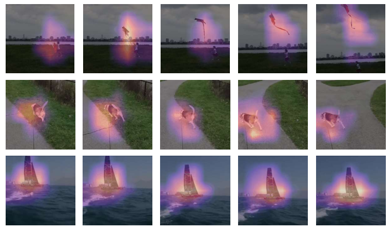
For a fair comparison, we slightly tune the hyperparameter to ensure their FLOPs and parameters to be similar. We report the accuracy of these variants on Kinetics-400 in the upper part of Table 4.2. Among these variants, (GG, GG, GG, GG) performs the worst since the local context information is very important to a patch. The model with only LW-MSA degrades by 1.1% top-1 score (79.5% $\rightarrow$ 78.4%) due to a limited receptive field at every stage. By integrating GP-MSA to increase the receptive field, both (LL, LL, LG, LG) and (LG, LG, LL, LL) achieve better performance than the variants with only local or global modules. In particular, adding GP-MSA to the early stages benefits more than late stages, revealing the importance of GP-MSA to complement the early stages. Moreover, we evaluate the two pyramid scales in GP-MSA and report their results in the lower part of Table 4.2. Compared to our default setting, we can find a clear accuracy drop by removing either the (4, 4, 4) or (8, 7, 7) scale. In addition, some examples of attention visualization are shown in Figure 4.2.

Effect of testing views. Previous methods employ multiple space-time views to boost performance during inference, e.g., 10 $\times$ 3 views in VidTr-L and 4 $\times$ 3 views in Swin. We investigate how the number of testing views affects the accuracy of DualFormer-T on Kinetics-400 and Diving-48. From Figure 6, one can find that increasing the number of temporal clips can bring significant improvement on both datasets, while using more spatial crops does not always help. For example, using three spatial crops slightly outperforms the 1-crop counterpart on Diving-48. As the inference FLOPs is proportional to the space-time views, to trade off the computational cost and accuracy, our method uses a testing strategy of four temporal clips with a spatial crop (totally four) during the inference phase.

Figure 6: Effect of space-time views on Kinetics-400 (left) and on Diving-48 (right).

Input Window Size FLOPs Top-1 Top-5 16 $\times$ 4 4 $\times$ 7 $\times$ 7 104 78.0 93.2 16 $\times$ 4 8 $\times$ 7 $\times$ 7 112 78.4 93.3 32 $\times$ 2 4 $\times$ 7 $\times$ 7 224 79.1 93.9 32 $\times$ 2 8 $\times$ 7 $\times$ 7 240 79.5 94.1 32 $\times$ 2 16 $\times$ 7 $\times$ 7 272 79.7 94.4 32 $\times$ 2 8 $\times$ 14 $\times$ 14 324 79.7 94.5 Table 7: Effect of window size of LW-MSA with DualFormer-T on Kinetic-400. The gray row indicates the default configuration. Method FLOPs Param Top-1 AvgPool 59 21.8 78.7 Conv 61 27.6 79.5 DWConv 60 21.8 79.5 Table 10: Results of pyramid downsampling functions based on DualFormer-T on Kinetics-400.

Effect of window size in LW-MSA. Window size is a crucial hyperparameter in LW-MSA. Hence, we test different window sizes to investigate their effect on model performance. As shown in Table 10, a larger window size in both temporal and spatial dimensions brings consistent gains in accuracy due to the increase of local receptive field, but also induces heavier computation. For an accuracy-speed balance, we choose $(8,7,7)$ as our default setting. From this table, we also observe that reducing the number of input frames (e.g., 32 $\rightarrow$ 16) can dramatically improve efficiency but inevitably degrades the top-1 accuracy by $\sim$ 1%.

Effect of pyramid downsampling function. There are several alternative functions to generate global priors in GP-MSA, such as average pooling (AvgPool) and standard convolution (Conv). Here, we replace the depth-wise convolution (DWConv) with them on Kinetics-400 to investigate their effect. As reported in Table 10, our DWConv achieves comparable performance to Conv while using much fewer parameters. Our implementation also outperforms AvgPool by 0.8% on the top-1 score with similar computation costs.

Do we need PEG? As depicted in Table 16, DualFormer without PEG suffers from a clear drop on the top-1 accuracy (79.5% $\rightarrow$ 78.9%), which indicates the necessity of integrating position information in MSA. We further compare our DWConv-based PEG with an absolute position encoding (i.e., TimeSformer) and a relative bias-based method in Swin. As a result, our solution achieves 0.3% and 0.2% higher top-1 score than the absolute and relative method, respectively.

Effect of Temporal Pooling Rate. Our method follows [11, 35] to utilize a multi-scale hierarchy. Such hierarchy is achieved by the patch merging layer at the beginning of the last three stages, where we downsample the spatial size of feature map by 2 $\times$ and keep the original temporal resolution. Here, we discuss the effect of temporal pooling at the last three stages. According to the results in Table 16, even though such temporal pooling can further reduce the computational cost, it also leads to a decrease in the overall accuracy.

Method Top-1 w.o PEG 78.9 Absolute [3] 79.2 Relative [35] 79.3 DWConv 79.5 Table 13: Effect of PEGs to DualFormer-T on the Kinetics-400 dataset. Rate Patch Size FLOPs Param Top-1 Top-5 $1,1,1$ $(4,4,4)$ 112 21.8 78.5 93.3 $2,1,1$ $(2,4,4)$ 136 21.8 78.7 93.5 $1,2,1$ $(2,4,4)$ 152 21.9 78.8 93.5 $1,1,2$ $(2,4,4)$ 216 22.3 79.2 93.9 $1,1,1$ $(2,4,4)$ 240 21.8 79.5 94.1 Table 16: Effect of temporal pooling in DualFormer-T on Kinetic-400. $(i,j,k)$ means reducing the temporal resolution $i$ , $j$ , $k$ times at the last 3 stages, respectively.

5 Conclusion

In this paper, we develop a transformer-based architecture with local-global attention stratification for efficient video recognition. Empirical study demonstrates that the proposed method achieves a better accuracy-speed trade-off on five popular video recognition datasets. In the future, we plan to remove the strong dependency on pretrained models and design a useful strategy to train our model from scratch. Another direction is to explore the use of our model in other applications, such as video segmentation and prediction.

Acknowledgement

We thank Quanhong Fu at Sea AI Lab for the help to improve the paper writing. This research is supported by Singapore Ministry of Education Academic Research Fund Tier 1 under MOE’s official grant number T1 251RES2029.

References

[1] Arnab, A., Dehghani, M., Heigold, G., Sun, C., Lučić, M., Schmid, C.: Vivit: A video vision transformer. arXiv preprint arXiv:2103.15691 (2021)
[2] Ba, J.L., Kiros, J.R., Hinton, G.E.: Layer normalization. arXiv preprint arXiv:1607.06450 (2016)
[3] Bertasius, G., Wang, H., Torresani, L.: Is space-time attention all you need for video understanding? arXiv preprint arXiv:2102.05095 (2021)
[4] Bulat, A., Perez-Rua, J.M., Sudhakaran, S., Martinez, B., Tzimiropoulos, G.: Space-time mixing attention for video transformer. arXiv preprint arXiv:2106.05968 (2021)
[5] Carreira, J., Zisserman, A.: Quo vadis, action recognition? a new model and the kinetics dataset. In: proceedings of the IEEE Conference on Computer Vision and Pattern Recognition. pp. 6299–6308 (2017)
[6] Chen, C.F., Panda, R., Fan, Q.: Regionvit: Regional-to-local attention for vision transformers. arXiv preprint arXiv:2106.02689 (2021)
[7] Chollet, F.: Xception: Deep learning with depthwise separable convolutions. In: Proceedings of the IEEE conference on computer vision and pattern recognition. pp. 1251–1258 (2017)
[8] Chu, X., Tian, Z., Wang, Y., Zhang, B., Ren, H., Wei, X., Xia, H., Shen, C.: Twins: Revisiting the design of spatial attention in vision transformers. In: NeurIPS 2021 (2021)
[9] Chu, X., Tian, Z., Zhang, B., Wang, X., Wei, X., Xia, H., Shen, C.: Conditional positional encodings for vision transformers. arXiv preprint arXiv:2102.10882 (2021)
[10] Dosovitskiy, A., Beyer, L., Kolesnikov, A., Weissenborn, D., Zhai, X., Unterthiner, T., Dehghani, M., Minderer, M., Heigold, G., Gelly, S., et al.: An image is worth 16x16 words: Transformers for image recognition at scale. In: International Conference on Learning Representations (2020)
[11] Fan, H., Xiong, B., Mangalam, K., Li, Y., Yan, Z., Malik, J., Feichtenhofer, C.: Multiscale vision transformers. arXiv preprint arXiv:2104.11227 (2021)
[12] Feichtenhofer, C.: X3d: Expanding architectures for efficient video recognition. In: Proceedings of the IEEE/CVF Conference on Computer Vision and Pattern Recognition. pp. 203–213 (2020)
[13] Feichtenhofer, C., Fan, H., Malik, J., He, K.: Slowfast networks for video recognition. In: Proceedings of the IEEE/CVF international conference on computer vision. pp. 6202–6211 (2019)
[14] Goyal, R., Ebrahimi Kahou, S., Michalski, V., Materzynska, J., Westphal, S., Kim, H., Haenel, V., Fruend, I., Yianilos, P., Mueller-Freitag, M., et al.: The” something something” video database for learning and evaluating visual common sense. In: Proceedings of the IEEE international conference on computer vision. pp. 5842–5850 (2017)
[15] Hara, K., Kataoka, H., Satoh, Y.: Learning spatio-temporal features with 3d residual networks for action recognition. In: Proceedings of the IEEE International Conference on Computer Vision Workshops. pp. 3154–3160 (2017)
[16] Hara, K., Kataoka, H., Satoh, Y.: Can spatiotemporal 3d cnns retrace the history of 2d cnns and imagenet? In: Proceedings of the IEEE conference on Computer Vision and Pattern Recognition. pp. 6546–6555 (2018)
[17] He, K., Zhang, X., Ren, S., Sun, J.: Deep residual learning for image recognition. In: Proceedings of the IEEE conference on computer vision and pattern recognition. pp. 770–778 (2016)
[18] Hongeng, S., Nevatia, R., Bremond, F.: Video-based event recognition: activity representation and probabilistic recognition methods. Computer Vision and Image Understanding 96(2), 129–162 (2004)
[19] Huang, G., Sun, Y., Liu, Z., Sedra, D., Weinberger, K.Q.: Deep networks with stochastic depth. In: European conference on computer vision. pp. 646–661. Springer (2016)
[20] Islam, M.A., Jia, S., Bruce, N.D.: How much position information do convolutional neural networks encode? arXiv preprint arXiv:2001.08248 (2020)
[21] Ji, S., Xu, W., Yang, M., Yu, K.: 3d convolutional neural networks for human action recognition. IEEE transactions on pattern analysis and machine intelligence 35(1), 221–231 (2012)
[22] Jiang, B., Wang, M., Gan, W., Wu, W., Yan, J.: Stm: Spatiotemporal and motion encoding for action recognition. In: Proceedings of the IEEE/CVF International Conference on Computer Vision. pp. 2000–2009 (2019)
[23] Jiang, Z., Hou, Q., Yuan, L., Zhou, D., Jin, X., Wang, A., Feng, J.: Token labeling: Training a 85.5% top-1 accuracy vision transformer with 56m parameters on imagenet. arXiv preprint arXiv:2104.10858 (2021)
[24] Karpathy, A., Toderici, G., Shetty, S., Leung, T., Sukthankar, R., Fei-Fei, L.: Large-scale video classification with convolutional neural networks. In: Proceedings of the IEEE conference on Computer Vision and Pattern Recognition. pp. 1725–1732 (2014)
[25] Kay, W., Carreira, J., Simonyan, K., Zhang, B., Hillier, C., Vijayanarasimhan, S., Viola, F., Green, T., Back, T., Natsev, P., et al.: The kinetics human action video dataset. arXiv preprint arXiv:1705.06950 (2017)
[26] Kingma, D.P., Ba, J.: Adam: A method for stochastic optimization. arXiv preprint arXiv:1412.6980 (2014)
[27] Krizhevsky, A., Sutskever, I., Hinton, G.E.: Imagenet classification with deep convolutional neural networks. Advances in neural information processing systems 25, 1097–1105 (2012)
[28] Kuehne, H., Jhuang, H., Garrote, E., Poggio, T., Serre, T.: Hmdb: a large video database for human motion recognition. In: 2011 International conference on computer vision. pp. 2556–2563. IEEE (2011)
[29] Li, K., Wang, Y., Peng, G., Song, G., Liu, Y., Li, H., Qiao, Y.: Uniformer: Unified transformer for efficient spatial-temporal representation learning. In: International Conference on Learning Representations (2021)
[30] Li, Y., Li, Y., Vasconcelos, N.: Resound: Towards action recognition without representation bias. In: Proceedings of the European Conference on Computer Vision (ECCV). pp. 513–528 (2018)
[31] Li, Z., Liu, F., Yang, W., Peng, S., Zhou, J.: A survey of convolutional neural networks: analysis, applications, and prospects. IEEE Transactions on Neural Networks and Learning Systems (2021)
[32] Lin, J., Gan, C., Han, S.: Tsm: Temporal shift module for efficient video understanding. In: Proceedings of the IEEE/CVF International Conference on Computer Vision. pp. 7083–7093 (2019)
[33] Lin, M., Chen, Q., Yan, S.: Network in network. In: Bengio, Y., LeCun, Y. (eds.) 2nd International Conference on Learning Representations, ICLR 2014, Banff, AB, Canada, April 14-16, 2014, Conference Track Proceedings (2014)
[34] Liu, Z., Lin, Y., Cao, Y., Hu, H., Wei, Y., Zhang, Z., Lin, S., Guo, B.: Swin transformer: Hierarchical vision transformer using shifted windows. International Conference on Computer Vision (ICCV) (2021)
[35] Liu, Z., Ning, J., Cao, Y., Wei, Y., Zhang, Z., Lin, S., Hu, H.: Video swin transformer. arXiv preprint arXiv:2106.13230 (2021)
[36] Liu, Z., Luo, D., Wang, Y., Wang, L., Tai, Y., Wang, C., Li, J., Huang, F., Lu, T.: Teinet: Towards an efficient architecture for video recognition. In: Proceedings of the AAAI Conference on Artificial Intelligence. vol. 34, pp. 11669–11676 (2020)
[37] Liu, Z., Wang, L., Wu, W., Qian, C., Lu, T.: Tam: Temporal adaptive module for video recognition. In: Proceedings of the IEEE/CVF International Conference on Computer Vision. pp. 13708–13718 (2021)
[38] Neimark, D., Bar, O., Zohar, M., Asselmann, D.: Video transformer network. arXiv preprint arXiv:2102.00719 (2021)
[39] Patrick, M., Campbell, D., Asano, Y.M., Metze, I.M.F., Feichtenhofer, C., Vedaldi, A., Henriques, J., et al.: Keeping your eye on the ball: Trajectory attention in video transformers. arXiv preprint arXiv:2106.05392 (2021)
[40] Qian, R., Meng, T., Gong, B., Yang, M.H., Wang, H., Belongie, S., Cui, Y.: Spatiotemporal contrastive video representation learning. In: Proceedings of the IEEE/CVF Conference on Computer Vision and Pattern Recognition. pp. 6964–6974 (2021)
[41] Qiu, Z., Yao, T., Mei, T.: Learning spatio-temporal representation with pseudo-3d residual networks. In: proceedings of the IEEE International Conference on Computer Vision. pp. 5533–5541 (2017)
[42] Ranftl, R., Bochkovskiy, A., Koltun, V.: Vision transformers for dense prediction. In: Proceedings of the IEEE/CVF International Conference on Computer Vision. pp. 12179–12188 (2021)
[43] Selvaraju, R.R., Cogswell, M., Das, A., Vedantam, R., Parikh, D., Batra, D.: Grad-cam: Visual explanations from deep networks via gradient-based localization. In: Proceedings of the IEEE international conference on computer vision. pp. 618–626 (2017)
[44] Simonyan, K., Zisserman, A.: Very deep convolutional networks for large-scale image recognition. arXiv preprint arXiv:1409.1556 (2014)
[45] Soomro, K., Zamir, A.R., Shah, M.: Ucf101: A dataset of 101 human actions classes from videos in the wild. arXiv preprint arXiv:1212.0402 (2012)
[46] Tobler, W.R.: A computer movie simulating urban growth in the detroit region. Economic geography 46(sup1), 234–240 (1970)
[47] Touvron, H., Cord, M., Douze, M., Massa, F., Sablayrolles, A., Jégou, H.: Training data-efficient image transformers & distillation through attention. In: International Conference on Machine Learning. pp. 10347–10357. PMLR (2021)
[48] Tran, D., Bourdev, L., Fergus, R., Torresani, L., Paluri, M.: Learning spatiotemporal features with 3d convolutional networks. In: Proceedings of the IEEE international conference on computer vision. pp. 4489–4497 (2015)
[49] Tran, D., Wang, H., Torresani, L., Feiszli, M.: Video classification with channel-separated convolutional networks. In: Proceedings of the IEEE/CVF International Conference on Computer Vision. pp. 5552–5561 (2019)
[50] Tran, D., Wang, H., Torresani, L., Ray, J., LeCun, Y., Paluri, M.: A closer look at spatiotemporal convolutions for action recognition. In: Proceedings of the IEEE conference on Computer Vision and Pattern Recognition. pp. 6450–6459 (2018)
[51] Vaswani, A., Shazeer, N., Parmar, N., Uszkoreit, J., Jones, L., Gomez, A.N., Kaiser, Ł., Polosukhin, I.: Attention is all you need. In: Advances in neural information processing systems. pp. 5998–6008 (2017)
[52] Wang, H., Zhu, Y., Adam, H., Yuille, A., Chen, L.C.: Max-deeplab: End-to-end panoptic segmentation with mask transformers. In: Proceedings of the IEEE/CVF Conference on Computer Vision and Pattern Recognition. pp. 5463–5474 (2021)
[53] Wang, L., Xiong, Y., Wang, Z., Qiao, Y., Lin, D., Tang, X., Van Gool, L.: Temporal segment networks for action recognition in videos. IEEE transactions on pattern analysis and machine intelligence 41(11), 2740–2755 (2018)
[54] Wang, W., Xie, E., Li, X., Fan, D.P., Song, K., Liang, D., Lu, T., Luo, P., Shao, L.: Pyramid vision transformer: A versatile backbone for dense prediction without convolutions. arXiv preprint arXiv:2102.12122 (2021)
[55] Wang, Y., Xu, Z., Wang, X., Shen, C., Cheng, B., Shen, H., Xia, H.: End-to-end video instance segmentation with transformers. In: Proceedings of the IEEE/CVF Conference on Computer Vision and Pattern Recognition. pp. 8741–8750 (2021)
[56] Wei, C., Fan, H., Xie, S., Wu, C.Y., Yuille, A., Feichtenhofer, C.: Masked feature prediction for self-supervised visual pre-training. arXiv preprint arXiv:2112.09133 (2021)
[57] Xie, S., Sun, C., Huang, J., Tu, Z., Murphy, K.: Rethinking spatiotemporal feature learning: Speed-accuracy trade-offs in video classification. In: Proceedings of the European conference on computer vision (ECCV). pp. 305–321 (2018)
[58] Xu, H., Das, A., Saenko, K.: R-c3d: Region convolutional 3d network for temporal activity detection. In: Proceedings of the IEEE international conference on computer vision. pp. 5783–5792 (2017)
[59] Yang, J., Li, C., Zhang, P., Dai, X., Xiao, B., Yuan, L., Gao, J.: Focal self-attention for local-global interactions in vision transformers. arXiv preprint arXiv:2107.00641 (2021)
[60] Zha, X., Zhu, W., Lv, T., Yang, S., Liu, J.: Shifted chunk transformer for spatio-temporal representational learning. arXiv preprint arXiv:2108.11575 (2021)
[61] Zhang, Y., Li, X., Liu, C., Shuai, B., Zhu, Y., Brattoli, B., Chen, H., Marsic, I., Tighe, J.: Vidtr: Video transformer without convolutions. In: Proceedings of the IEEE/CVF International Conference on Computer Vision. pp. 13577–13587 (2021)
[62] Zhu, X., Su, W., Lu, L., Li, B., Wang, X., Dai, J.: Deformable detr: Deformable transformers for end-to-end object detection. arXiv preprint arXiv:2010.04159 (2020)