Lepton-Flavor-Violating ALPs at the Electron-Ion Collider: A Golden Opportunity

Global symmetries arise in a variety of theoretical settings and their spontaneous breaking generally leads to axion-like particles (ALPs) Peccei:1977hh; Weinberg:1977ma; Wilczek:1977pj; Georgi:1986df. Often the global symmetry is not exact and its small explicit breaking leads to the appearance of relatively light ALPs. In the Standard Model (SM), the spontaneous breaking of chiral symmetries gives rise to pseudo-Nambu-Goldstone bosons, i.e. the parity-odd pions, which have axion-like properties. The small masses of light quarks, compared to typical hadronic scale $\Lambda_{\rm QCD}\sim 200$ MeV, provide explicit chiral symmetry breaking, leading to relatively small pion masses.

One may expect similar phenomena to arise in new sectors of physics, which could provide answers for open questions like the nature of dark matter (DM), for example. New physics sectors at scales of $\mathcal{O}{(\rm GeV)}$ or less have been considered as potential alternatives to beyond SM (BSM) models at or above the weak scale $\sim 100$ GeV. In particular, “dark sectors” that could include DM and other related states and interactions have been extensively studied over the last several years. In these setups, new experimental possibilities for discovery of BSM phenomena open up. Due to the relatively low scale and feeble couplings associated with such “dark sectors,” intense sources can provide good prospects for uncovering them.

Searches for lepton flavor violation (LFV) mediated by ALPs can be a particularly sensitive probe of new physics Wilczek:1982rv; Ema:2016ops; Bauer:2019gfk; Cornella:2019uxs; Endo:2020mev; Iguro:2020rby; Han:2020dwo; Mukaida:2021sgv; Bauer:2021mvw. For an example of a concrete UV-complete model in which GeV-scale ALPs with lepton flavor violation emerge out of a dark sector giving rise to dark matter and neutrino mass, see Refs. Davoudiasl:2017zws. The dominant current constraints on flavor off-diagonal ALP-lepton couplings universally come from low-energy experimental searches involving flavor-violating lepton decays Cornella:2019uxs; Bauer:2021mvw, such as $\tau\rightarrow e\mu\mu$ for the $ae\tau$ interaction, where $a$ denotes the ALP. Searches for ALPs produced in Higgs decays can also provide relevant limits Davoudiasl:2021haa, particularly for relatively heavy ALP masses above 2 GeV. However, these experimental probes require the existence of other significant couplings - either flavor-diagonal interactions $a\ell\ell$ or ALP-Higgs couplings - in addition to the flavor-violating couplings. In particular, the constraints from lepton decays become sharply weaker for axion masses above the tau lepton mass, where the decays become highly suppressed due to kinematics.

One may also consider $Z$ decays as a probe of ALP mediated LFV at the LHC. Assuming the $a$-$e$-$\tau$ coupling $C_{\tau e}/\Lambda\lesssim 10$ TeV^-1 (typical of the parameter space in our analysis below) only and for $m_{a}\ll m_{Z}$, we estimate that gives a branching fraction

for which no experimental bounds exist at the present (the current measurement of 4-lepton $Z$ decays has an uncertainty of $\sim 2\times 10^{-7}$ ParticleDataGroup:2020ssz, but only applies to electron and muon final states). Though not directly relevant, we also note that the limit on flavor-violating $Z\to e\tau$ decay branching fractions is $5\times 10^{-6}$ at 95% confidence level ParticleDataGroup:2020ssz. In any event, it could be interesting to consider bounds from $Z$ decays in more detail in future work.

Motivated by the above considerations, in this work, we examine the possibility of probing lepton-flavor-violating ALPs arising at or above the GeV scale, perhaps as part of a new dark sector of physics, in electron-ion collisions at the future Electron-Ion Collider (EIC). We will focus specifically on probing the $ae\tau$ interaction through the process $e\rightarrow\tau a$. In contrast with bounds on this interaction from rare lepton decays, the EIC is directly sensitive to the $ae\tau$ coupling with no requirement of significant flavor-diagonal lepton couplings. Compared to electron-proton scattering experiments, electron-ion collisions offer a coherent enhancement in scattering rate due to the ion charge, increasing the ALP production rate in electromagnetic scattering processes by orders of magnitude (although this enhancement is partially compensated by reduced ion luminosity compared to electron-proton operation.) These features, along with its high center-of-mass energy, make the EIC uniquely effective at searching for LFV ALPs in theoretically interesting regions of parameter space. Additionally, the use of beam polarization at the EIC provides an experimental handle on the parity-violating angle in the $ae\tau$ interaction.

In this paper, we will study the ALP EFT allowing for both LFV and parity non-conservation. Exploiting the presence of LFV, we will focus on tau lepton final states. Under a wide range of efficiency assumptions, we will estimate projected limits on the $ae\tau$ interaction and compare with existing bounds. Other works that consider exploring LFV using electron beam facilities include Ref. Gonderinger:2010yn; Cirigliano:2021img; Zhang:2022zuz (EIC) and Ref. Furletova:2021wyq (CEBAF), where a leptoquark sector is generally assumed to mediate the effects studied therein. Recent work Liu:2021lan has also studied the prospects for detecting ALPs through their photon coupling at the EIC.

The flavor-violating ALP effective Lagrangian we will adopt for this analysis has been previously considered in Refs. Bauer:2017ris; Cornella:2019uxs; Bauer:2019gfk; Bauer:2020jbp; Chala:2020wvs; Escribano:2020wua; Calibbi:2020jvd; Ma:2021jkp; Bauer:2021mvw. It is given by

where $\Lambda$ is the EFT scale of the ALP theory. Here, we will take $V_{\ell\ell^{\prime}}$ and $A_{\ell\ell^{\prime}}$ to be real, so that the Lagrangian is CP-even. However, note that the presence of the vector-like $V_{\ell\ell^{\prime}}$ term implies that parity violation is present in general. The parity violation can be parametrized by an angle $\theta_{\ell\ell^{\prime}}$ by defining $\theta_{\ell\ell^{\prime}}=-\tan^{-1}(V_{\ell\ell^{\prime}}/A_{\ell\ell^{\prime}})$ and $C_{\ell\ell^{\prime}}=\sqrt{V_{\ell\ell^{\prime}}^{2}+A_{\ell\ell^{\prime}}^{2}}$, so that

Note that $\theta_{\ell\ell^{\prime}}=0$ leaves only the parity-even term, while $\theta_{\ell\ell^{\prime}}=\pi/4$ ($\theta_{\ell\ell^{\prime}}=3\pi/4$) is maximally parity-violating, because then the ALP only interacts with left-handed (right-handed) particles.

It is useful to rewrite the leptonic Lagrangian by integrating by parts and solving the classical equations of motion on the leptons. Doing so, we have

where $m^{\pm}\equiv m_{\ell}\pm m_{\ell^{\prime}}$. Here, we note that there is no PV contribution for the flavor-diagonal case, because for $\ell=\ell^{\prime}$, the difference in masses goes to zero, so we can absorb $\cos\theta_{\ell\ell}$ into the definition of $C_{\ell\ell}$. Although we will neglect $\theta_{\ell\ell}$, it is worth noting that the presence of parity violation will tend to suppress the diagonal couplings $|C_{\ell\ell}|$ relative to the off-diagonal couplings $|C_{\ell\ell^{\prime}}|$. We will retain the explicit dependence on parity violation in the off-diagonal couplings, although we will find that this dependence vanishes in our signal cross-section.

The above model could lead to an interesting LFV (and potentially parity violating) signal at the EIC. In particular, one can consider the process in Fig. (1), where the coupling $C_{\tau e}$ allows for the process $eA_{Z}\rightarrow\tau A_{Z}a$, emission of an ALP in which the beam electron is converted to a tau lepton. The emitted $a$ can then decay into leptonic final states.

We restrict our attention to the $\tau$ lepton because of the mass-dependence of the ALP coupling: since $m_{\tau}\gg m_{\mu}\gg m_{e}$, the branching fractions into final states containing only $\mu$ and $e$ are negligible. We further neglect the $C_{\tau\mu}$ coupling, for two reasons: first, the $C_{\tau e}$ coupling is essential for the production of our ALP signal, whereas $C_{\tau\mu}$ will only be relevant for ALP decays; second, current plans for the EIC detectors do not necessarily include muon chambers, in which case muonic decays of the ALP will be difficult to detect. In this scenario, the only terms in the Lagrangian we are interested in are those which contain at least one $\tau$; in particular,

where $m_{e}$ is ignored. For $m_{a}>m_{\tau}\gg m_{e}$, the decay rates of interest are

For the region of parameter space explored in this paper, the $a$ decay is always prompt. We restrict our attention to $m_{a}>m_{\tau}+m_{e}$; as shown in Fig. 3 below, other bounds on the $|C_{\tau e}|$ coupling become much stronger for $m_{a}<m_{\tau}$.

We are now in a position to evaluate the diagram in Fig. (1). The incoming momenta are denoted as $p^{\mu}$ for the electron and $P_{i}^{\mu}$ for the incoming ion, and the outgoing momenta are denoted as $p^{\prime\mu}$ for the $\tau$, $k$ for the ALP, and $P_{f}^{\mu}$ for the outgoing ion. We restrict our attention to events in which the interaction with the ion is coherent and elastic, i.e. the ion does not break apart; these events will give the dominant contribution to our signal due to the $Z^{2}$ enhancement discussed below. The four-momentum of the exchanged photon is given by $q^{\mu}\equiv P_{i}^{\mu}-P_{f}^{\mu}$. For simplicity (following Refs. Liu:2016mqv; Liu:2017htz), we will assume that the ion is a scalar boson with mass $M$, atomic number $Z$, and form factor $F(q^{2})$, so that the interaction of a photon with the ion is

From here forward, we will specialize to a gold ion ($Z=79$, mass number $A=197$), corresponding to a mass of $M=183$ GeV. The form factor is an approximation of the Fourier transform of the Woods-Saxon distribution applied to the gold nucleus Klein:1999qj, given by

where $a_{0}=0.79~{\rm fm}$, $R_{A}=(1.1~{\rm fm})A^{1/3}$. For low momentum transfer, $F(q^{2})\approx 1$, so the amplitude is proportional to $Z$. As a result, the cross section will be enhanced by a factor of $79^{2}\approx 6000$ for small momentum transfer. This $Z^{2}$ enhancement enables the constraints made on $C_{\tau e}$ to be competitive with existing constraints, as we discuss below. We have found, through numerical inspection, that $F(q)\sim 1$ until $m_{a}\sim 20$ GeV, corresponding to the region with the above $Z^{2}$ enhancement. Above this mass scale, $F(q)<1$ and decreases with larger $m_{a}$, leading to a suppressed ALP production cross section. To restrict to the signal region where nuclear breakup does not occur, we additionally require a cutoff in the form factor of $q^{2}<(100~{\rm MeV})^{2}$, corresponding to $m_{a}\sim 27~{\rm GeV}$.

To compute the amplitude, it is useful to define some Mandelstam-like variables in terms of the momenta of the diagram. We have

The amplitude calculation is done in full detail in Appendix A; the final spin-averaged result is given by

where $\alpha$ is the fine-structure constant, and

where $M^{2}(\theta_{\tau e})=m_{a}^{2}-m_{\tau}^{2}-m_{e}^{2}+2m_{\tau}m_{e}\cos{(2\theta_{\tau e})}$. Note that for the spin-averaged amplitude, the only dependence on the parity violating angle $\theta_{\tau e}$ is an ${\cal O}(m_{e}/m_{\tau})$ correction to the amplitude, so to very good precision one can compute the spin-averaged cross-section with $\overline{|{\cal A}_{0}|^{2}}\equiv\overline{|{\cal A}|^{2}}(\theta_{\tau e}=0)$. We find that these results are in agreement with Refs. Liu:2016mqv; Liu:2017htz with the replacement $m_{\tau}\rightarrow m_{e}$ (any apparent sign discrepancies are due to the choice of the metric, which we take to be mostly negative).

To compute the cross section, the integral over phase space is also done following Ref. Liu:2017htz closely. Defining $x=E_{k}/|\bf p|$ to be the fraction of energy the ALP has w.r.t. the electron (assuming $p^{0}=|{\bf p}|$), the differential cross-section in the rest frame of the ion is given by

where $V=|{\bf V}|=|{\bf p}-{\bf k}|$, $\theta_{k}$ is the angle ${\bf k}$ makes with ${\bf p}$, $\phi_{q}$ is the azimuthal angle of ${\bf q}$ about ${\bf V}$, and $t_{\pm}$ are kinematic bounds from the energy-conserving $\delta$-function in the Lorentz-invariant phase space. Details on the phase-space calculation are given in the Appendix B.

In order to evaluate the phase-space integral, we must determine the values of the initial-state momenta in Fig. (1). For this, we use Table 10.2 of the EIC Yellow Report AbdulKhalek:2021gbh, which states that the highest energies for the electron and gold ion beams are $|{\bf p}^{\rm lab}|=18\,\textrm{GeV}$ and $E_{i}^{\rm lab}=110\,\textrm{GeV}/{\rm nucleon}$, respectively. In the rest frame of the gold ion, a relativistic calculation reveals that the electron momentum has a magnitude of $|{\bf p}|\approx 4200\,\textrm{GeV}$.

Next, we must determine the range of integration for $\cos\theta_{k}$. Following the detector requirements listed in Table 10.6 of the EIC Yellow Report, we assume a detector pseudorapidity range of $|\eta|<3.5$, corresponding to a range of angles $0.04<\theta^{\rm lab}<\pi-0.04$ in the lab frame. For most of the phase-space of interest, the differential cross-section in Eq. 16 is highly peaked near $\theta=0$, making numerical integration challenging. This can be remedied by transforming from $\cos{\theta_{k}}$ to $\eta$, with the added benefit that one can then directly integrate over the allowed pseudorapidity region. The details of this transformation are shown in the Appendix B.

After inserting the kinematic parameters and doing the relevant transformations described above, the integral can be evaluated. The $\phi_{q}$ integrals are computed analytically, and the rest are done via trapezoid integration. The result for the total cross-section integration are shown in Fig. (2).

Finally, we comment on the effect of beam polarization on the ALP signal. To compute the polarized amplitude or cross-section, there are slight modifications to be made. In particular, one can rewrite the $\tau e$ coupling as

where $R(\theta)=\cos{\theta}-\sin{\theta}$ and $L(\theta)=\cos{\theta}+\sin{\theta}$. The left-polarized cross-section can then be obtained by singling out the left-handed piece of Eq. (17). This simply corresponds to setting $\theta_{\tau e}=\pi/4$, then multiplying by $\frac{1}{\sqrt{2}}L(\theta_{\tau e})$. Hence, we find

where have used $\overline{|{\cal A}(\theta_{\tau e}=\pi/4)|^{2}}=2\overline{|{\cal A}(\theta_{\tau e}=\pi/4)|^{2}}\approx 2\overline{|{\cal A}_{0}|^{2}}$. The additional factor of 2 accounts for the fact that $\overline{|{\cal A}|^{2}}$ is a spin-averaged quantity. We similarly obtain

Hence, to good approximation, $\sigma_{L}=|L(\theta_{\tau e})|^{2}\sigma_{0}$ and $\sigma_{R}=|R(\theta_{\tau e})|^{2}\sigma_{0}$, where $\sigma_{0}$ represents the spin-averaged cross-section when $\theta_{\tau e}=0$. This allows us to compute the left-right asymmetry:

Observation of an ALP signal at varying beam polarizations can thus be used as a direct probe of the parity-violating angle $\theta_{\tau e}$.

Once the cross section is determined for a large sample of masses, limits can be placed on the coupling $C_{\tau e}$. Since the process always has an $ae\tau$ vertex, the cross section is proportional to $|C_{\tau e}|^{2}/\Lambda^{2}$. As a result, one can write the cross section as

In what follows, we will assume that the ALP always decays leptonically in the detector and that $m_{a}>m_{\tau}$. We note that the addition of the coupling $C_{\tau\mu}$ may enhance the ability to detect LFV at the EIC, but we avoid this scenario for more straightforward comparison with the LFV constraints from Ref. Cornella:2019uxs (and the possible lack of a dedicated muon detection capability, as mentioned earlier). Due to the mass-dependence of the ALP coupling, there are only three significant decay channels for the ALP: (i) $a\rightarrow\tau^{-}\tau^{+}$, (ii) $a\rightarrow\tau^{-}e^{+}$ and (iii) $a\rightarrow\tau^{+}e^{-}$.

Here, we note that the most advantageous aspect of our proposal for investigating LFV at the EIC is the ability to probe the $C_{\tau e}$ coupling nearly independently of the flavor-diagonal $C_{\tau\tau}$ coupling. In particular, when the latter is relatively suppressed, we find that the EIC can provide a promising venue for accessing the former. In that case, the final states of interest are $a(\rightarrow e^{\pm}\tau^{\mp})\tau^{-}$, on which we will focus. In particular, for our search, we will require the identification of an $e^{+}$ and a $\tau^{\pm}$ in the final state, and we will veto on the identification of an $e^{-}$. The largest source of irreducible background would then arise from electromagnetic production of $\tau$ pairs, which will be dominated by production through the Bethe-Heitler process Bethe:1934za; Ganapathi:1978qm; Akhundov:1979bd. To estimate this cross-section, we rescale the cross-sections found in Ref. Bulmahn:2008fa, which investigates the cross-section of ditau production from high-energy muons. We expect the difference between muon and electron collisions to be negligible for sufficiently high incident energies. We take the results are found for “rock” ($Z=11$, $A=22$) and rescale the cross-section by $(Z_{\rm Au}/Z_{\rm rock})^{2}=51$. For an incident beam energy of $E=4200\,{\rm GeV}$, this corresponds to a cross-section of $\sigma_{\rm b.g.}=2.6\times 10^{4}~{\rm pb}$. For $\tau$ identification, we will adopt the $\tau$ efficiency found in Ref. Zhang:2022zuz of $\epsilon_{\tau}\approx 1\%$, which only considers 3-pronged decays, though we note that this is completely ignoring the other $\tau$ decay modes and an improved analysis could likely give a higher efficiency. We also expect that one could improve the efficiency from the 3-pronged channel by vetoing on breakup of the ion, since this choice has no effect on our signal but reduces hadronic background. To calculate the background efficiency, we take a rate of $\sim 10^{-2}$ for losing the initial-state electron completely AbdulKhalek:2021gbh and a rate of $\sim 10^{-3}$ for misidentification of the $e^{-}$ as an $e^{+}$, in line with studies of pions faking an electron from AbdulKhalek:2021gbh. Then, the overall background efficiency is

where the first term comes from misidentifying the electron as a positron (and assumes the $\tau^{-}$ does not decay to $e^{-}$), and the second term comes from losing the electron down the beam-pipe and detecting a positron from the decay of the $\tau^{+}$. Hence, the number of expected background events with ${\cal L}=(100/A)~{\rm fb}^{-1}$ of integrated luminosity is $n_{\rm b.g.}=\epsilon_{\rm b.g.}\sigma_{\rm b.g.}{\cal L}\approx 475$. Following the analysis done in Ref. Feldman:1997qc, the upper end of the 90% confidence interval for Poisson signal mean given 475 mean background events and 475 observed events is $n_{\rm max}=35$. Hence, for a signal with acceptance$\times$efficiency $\epsilon$, a value of $C_{\tau e}$ can be ruled out at a 90% C.L. if

Here, the signal efficiency $\epsilon$ can be written as

where $\epsilon_{i}$ represent the individual efficiencies of each possible branching. Adopting the same $\tau$ efficiency and positron misidentification rate, we have $\epsilon_{1}=2(0.01)(0.82)\approx 0.016$, and $\epsilon_{2}=2(0.01)(0.82)(0.18)\approx 0.003$.

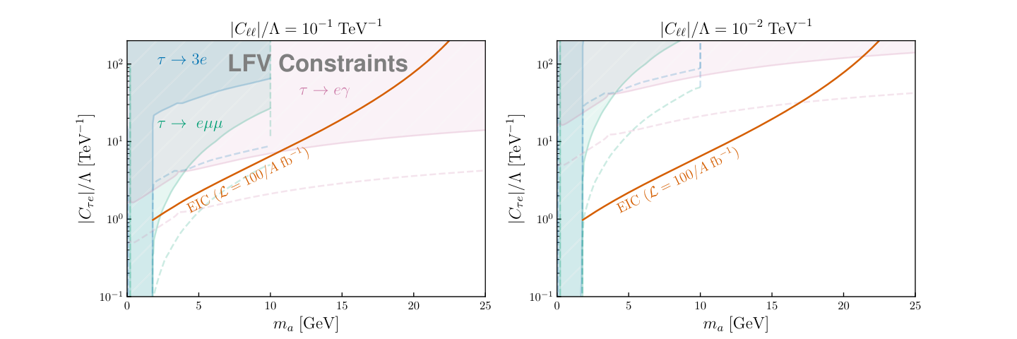
The panels in Fig. (3) show the effect of assuming diagonal ALP couplings equal to $C_{\ell\ell}/\Lambda=10^{-1}$ and $10^{-2}$ TeV^-1. Note that as $|C_{\ell\ell}|$ is reduced, our EIC production cross section remains unchanged, since it is only sensitive to $C_{\tau e}$. As a result, our proposal for exploring the $C_{\tau e}$ LFV coupling can far exceed future projections using other probes, particularly when $C_{\ell\ell}$ is small and other indirect searches are less constraining. The bounds obtained in the EIC search generally fall in a region of parameter space where $C_{\tau e}$ is significantly larger than $C_{\ell\ell}$; this may be realized in a general framework, or in the presence of significant parity violation as discussed above.

Axion-like particles (ALPs) appear in a wide range of physical settings and may play a role in explaining some of the open questions of particle physics. As such, they are well-motivated subjects of inquiry for theory and experiment. In this work, we considered ALPs, at or above the GeV scale, whose couplings can lead to lepton-flavor-violation (LFV) and may even dominate their interactions with the SM. We focused on $\tau-e$ LFV and showed that even with a fairly conservative analysis that does not make use of detailed kinematic information, the planned Electron-Ion Collider (EIC) can provide useful limits for this interaction, particularly in the case where the lepton-flavor-conserving couplings are suppressed. This is mostly due to two factors: (i) a significant coherent enhancement of low-momentum-transfer electromagnetic scattering from a large $Z$ ion, mediating ALP emission, and (ii) the sizeable center-of-mass energy $\sim 100$ GeV envisioned for the EIC allowing it to reach for ALPs well above the GeV scale. The final reach of such a search will depend on the EIC detectors’ efficiency for $\tau$ identification, which may be significantly improved if muon detection capabilities are included in their final design Adkins:2022jfp.

The EIC can reach beyond current and projected bounds for $\tau-e$ LFV in tau decays for ALP masses above $m_{\tau}$ up to $m_{a}\sim 20$ GeV, assuming universal diagonal lepton couplings of order $|C_{\ell\ell}|/\Lambda\lesssim 0.1\,\textrm{TeV}^{-1}$, with (100/A) fb^-1 of gold ion scattering data. The kinematics of the EIC are particularly favorable for production of ALPs towards the heavier end of this mass range, as opposed to fixed-target experiments Bjorken:2009mm; Liu:2017htz which benefit from high luminosity and similar $Z^{2}$ enhancement, but have much lower collision energy. A possible future fixed-target experiment using an ion beam at the LHC Hadjidakis:2018ifr could possibly provide competitive limits to the EIC and is worth future study.

One notable observation is that the limits on $C_{\tau e}$ from the EIC are more robust and model-independent than other limits. Although we have focused on LFV constraints, this is generally true. For example, similar constraints were found for a universal $a\ell\ell^{\prime}$ coupling by analyzing Higgs decays at the LHC in Ref. Davoudiasl:2021haa. These constraints were significantly weakened as the ALP-Higgs coupling was decreased, whereas the limits from the EIC would remain unaffected.

We also considered the possibility that ALPs may mediate parity-violating interactions. This, for example, can be realized in certain models with composite ALPs from new strong dynamics. Here, the EIC electron beam polarization can be a powerful probe of such interactions, making it a unique tool for illuminating the physics underlying LFV processes.

In principle, one could consider probing the muon-electron coupling $C_{\mu e}$ at the EIC using a similar search. However, the characteristic mass dependence of ALP couplings reduces the corresponding cross section by $(m_{\mu}/m_{\tau})^{2}$, so that an EIC search would not typically be competitive with other LFV bounds Cornella:2019uxs on $C_{\mu e}$, barring very small lepton-flavor diagonal $a\ell\ell$ and $a\gamma\gamma$ couplings. Production of ALPs via the third LFV coupling $C_{\tau\mu}$ is not accessible in electron-ion collisions, but if both $C_{\tau e}$ and $C_{\tau\mu}$ are significant then $a\rightarrow\mu\tau$ decays could provide access to the latter coupling, assuming that muon detection capabilities are included in the EIC detectors.

We thank Nicholas Miesch for helpful discussions in the early stages of this work, and Craig Woody for useful comments. This work is supported by the U.S. Department of Energy under Grant Contracts DE-SC0012704 (H. D.) and DE-SC0010005 (E. N. and R. M.).

References

- (1) R. D. Peccei and H. R. Quinn, CP Conservation in the Presence of Instantons, Phys. Rev. Lett. 38 (1977) 1440–1443.
- (2) S. Weinberg, A New Light Boson?, Phys. Rev. Lett. 40 (1978) 223–226.
- (3) F. Wilczek, Problem of Strong and Invariance in the Presence of Instantons, Phys. Rev. Lett. 40 (1978) 279–282.
- (4) H. Georgi, D. B. Kaplan, and L. Randall, Manifesting the Invisible Axion at Low-energies, Phys. Lett. B 169 (1986) 73–78.
- (5) F. Wilczek, Axions and Family Symmetry Breaking, Phys. Rev. Lett. 49 (1982) 1549–1552.
- (6) Y. Ema, K. Hamaguchi, T. Moroi, and K. Nakayama, Flaxion: a minimal extension to solve puzzles in the standard model, JHEP 01 (2017) 096, [arXiv:1612.05492].
- (7) M. Bauer, M. Neubert, S. Renner, M. Schnubel, and A. Thamm, Axionlike Particles, Lepton-Flavor Violation, and a New Explanation of and , Phys. Rev. Lett. 124 (2020), no. 21 211803, [arXiv:1908.00008].
- (8) C. Cornella, P. Paradisi, and O. Sumensari, Hunting for ALPs with Lepton Flavor Violation, JHEP 01 (2020) 158, [arXiv:1911.06279].
- (9) M. Endo, S. Iguro, and T. Kitahara, Probing flavor-violating ALP at Belle II, JHEP 06 (2020) 040, [arXiv:2002.05948].
- (10) S. Iguro, Y. Omura, and M. Takeuchi, Probing flavor-violating solutions for the muon anomaly at Belle II, JHEP 09 (2020) 144, [arXiv:2002.12728].
- (11) C. Han, M. L. López-Ibáñez, A. Melis, O. Vives, and J. M. Yang, Anomaly-free leptophilic axionlike particle and its flavor violating tests, Phys. Rev. D 103 (2021), no. 3 035028, [arXiv:2007.08834].
- (12) K. Mukaida, K. Schmitz, and M. Yamada, Leptoflavorgenesis: baryon asymmetry of the Universe from lepton flavor violation, arXiv:2111.03082.
- (13) M. Bauer, M. Neubert, S. Renner, M. Schnubel, and A. Thamm, Flavor probes of axion-like particles, arXiv:2110.10698.
- (14) H. Davoudiasl, P. P. Giardino, E. T. Neil, and E. Rinaldi, Unified Scenario for Composite Right-Handed Neutrinos and Dark Matter, Phys. Rev. D 96 (2017), no. 11 115003, [arXiv:1709.01082].
- (15) H. Davoudiasl, R. Marcarelli, N. Miesch, and E. T. Neil, Searching for Flavor-Violating ALPs in Higgs Decays, arXiv:2105.05866.
- (16) Particle Data Group Collaboration, P. A. Zyla et al., Review of Particle Physics, PTEP 2020 (2020), no. 8 083C01.
- (17) M. Gonderinger and M. J. Ramsey-Musolf, Electron-to-Tau Lepton Flavor Violation at the Electron-Ion Collider, JHEP 11 (2010) 045, [arXiv:1006.5063]. [Erratum: JHEP 05, 047 (2012)].
- (18) V. Cirigliano, K. Fuyuto, C. Lee, E. Mereghetti, and B. Yan, Charged Lepton Flavor Violation at the EIC, JHEP 03 (2021) 256, [arXiv:2102.06176].
- (19) J. L. Zhang et al., Search for Charged Lepton Flavor Violation at the EIC with the ECCE Detector, arXiv:2207.10261.
- (20) Y. Furletova and S. Mantry, Probing charged lepton flavor violation with a positron beam at CEBAF (JLAB), arXiv:2111.03912.
- (21) Y. Liu and B. Yan, Searching for the axion-like particle at the EIC, arXiv:2112.02477.
- (22) M. Bauer, M. Neubert, and A. Thamm, Collider Probes of Axion-Like Particles, JHEP 12 (2017) 044, [arXiv:1708.00443].
- (23) M. Bauer, M. Neubert, S. Renner, M. Schnubel, and A. Thamm, The Low-Energy Effective Theory of Axions and ALPs, arXiv:2012.12272.
- (24) M. Chala, G. Guedes, M. Ramos, and J. Santiago, Running in the ALPs, Eur. Phys. J. C 81 (2021), no. 2 181, [arXiv:2012.09017].
- (25) P. Escribano and A. Vicente, Ultralight scalars in leptonic observables, JHEP 03 (2021) 240, [arXiv:2008.01099].
- (26) L. Calibbi, D. Redigolo, R. Ziegler, and J. Zupan, Looking forward to Lepton-flavor-violating ALPs, arXiv:2006.04795.
- (27) K. Ma, Polarization Effects in Lepton Flavor Violated Decays Induced by Axion-Like Particles, arXiv:2104.11162.
- (28) Y.-S. Liu, D. McKeen, and G. A. Miller, Validity of the Weizsäcker-Williams approximation and the analysis of beam dump experiments: Production of a new scalar boson, Phys. Rev. D 95 (2017), no. 3 036010, [arXiv:1609.06781].
- (29) Y.-S. Liu and G. A. Miller, Validity of the Weizsäcker-Williams approximation and the analysis of beam dump experiments: Production of an axion, a dark photon, or a new axial-vector boson, Phys. Rev. D 96 (2017), no. 1 016004, [arXiv:1705.01633].
- (30) S. Klein and J. Nystrand, Exclusive vector meson production in relativistic heavy ion collisions, Phys. Rev. C 60 (1999) 014903, [hep-ph/9902259].
- (31) R. Abdul Khalek et al., Science Requirements and Detector Concepts for the Electron-Ion Collider: EIC Yellow Report, arXiv:2103.05419.
- (32) H. Bethe and W. Heitler, On the Stopping of fast particles and on the creation of positive electrons, Proc. Roy. Soc. Lond. A 146 (1934) 83–112.
- (33) V. Ganapathi and J. Smith, Electromagnetic Production of Trimuons in Deep Inelastic Muon Scattering, Phys. Rev. D 19 (1979) 801–809.
- (34) A. A. Akhundov, D. Y. Bardin, N. D. Gagunashvili, and N. M. Shumeiko, Electromagnetic Trident Production in Deep Inelastic Scattering, Sov. J. Nucl. Phys. 31 (1980) 127.
- (35) A. Bulmahn and M. H. Reno, Cross sections and energy loss for lepton pair production in muon transport, Phys. Rev. D 79 (2009) 053008, [arXiv:0812.5008].
- (36) G. J. Feldman and R. D. Cousins, A Unified approach to the classical statistical analysis of small signals, Phys. Rev. D 57 (1998) 3873–3889, [physics/9711021].
- (37) J. K. Adkins et al., Design of the ECCE Detector for the Electron Ion Collider, arXiv:2209.02580.
- (38) J. D. Bjorken, R. Essig, P. Schuster, and N. Toro, New Fixed-Target Experiments to Search for Dark Gauge Forces, Phys. Rev. D 80 (2009) 075018, [arXiv:0906.0580].
- (39) C. Hadjidakis et al., A fixed-target programme at the LHC: Physics case and projected performances for heavy-ion, hadron, spin and astroparticle studies, Phys. Rept. 911 (2021) 1–83, [arXiv:1807.00603].
Appendix A Amplitude Calculation
In computing the amplitude, we borrow notation from Refs. Liu:2016mqv; Liu:2017htz. In this appendix, we attempt to provide the amplitude calculation in as much detail as possible, stating explicitly whenever a computer algebra system was used.
Let the incoming four-momenta be for the electron and for the incoming ion. Let the outgoing momenta be for the , for the ALP, and for the outgoing ion. Also, let the mass of the ALP be , the mass of the ion be , and the charge of the ion be . We define and , along with the following Mandelstam variables: