Intertwining of lasing and superradiance under spintronic pumping Preprint: APS/123-QED

Introduction. The theme of dynamical phase transitions enabled by the interplay of interactions, drive, and dissipation permeates different branches of quantum many body physics, such as quantum optics Carusotto and Ciuti 2013; Stitely et al. 2020, cold atoms Ritsch et al. 2013, and non-equilibrium solid state physics Houck et al. 2012; Kirilyuk et al. 2010; Kessler et al. 2012. The interest in them ranges from practical applications in dynamical control to the fundamentals of statistical mechanics. The exploration and understanding of non-equilibrium phases would benefit from a unifying language, which, however, remains elusive due to the diversity of microscopic ingredients, relevant scales, and engineering capabilities across the various platforms.

In this Letter, we take a first step in filling this gap by studying a barebones model that offers complementary interpretations pertinent both to spintronics and driven-dissipative quantum optics, as illustrated in Fig. 1(a). We analyse a spin ensemble where coherent dynamical responses ascribable to lasing can be induced by weak coupling to a subsystem incoherently pumped into a population inverted regime. The model can be realized in an optical cavity, where two species of atoms, $\mathcal{S}$ and $\mathcal{T}$, are coupled to each other as well as to a common lossy cavity mode [cf. Fig. 1(b)]. The ensemble $\mathcal{S}$ collectively couples to the cavity photon via a Dicke term, while the ensemble $\mathcal{T}$ does via a spin-boson interconversion term. Dynamical instabilities can be induced in the subsystem $\mathcal{S}$ by incoherently spin pumping the subsystem $\mathcal{T}$, even in a limit of weak coupling between them. The interplay of the spin pumping and the Dicke coupling opens a parameter space where lasing and superradiant phases intertwine and lead to novel dynamical regimes exhibiting features of both.

Our motivation to separate the coherent ($\mathcal{S}$) and incoherent ($\mathcal{T}$) spin subsystems stems from a solid-state viewpoint, to allow quantum correlations to settle in without much disruption from direct pumping processes. Considering magnet-metal heterostructures Hauser 1969; Saitoh et al. 2006; Uchida et al. 2010; Kajiwara et al. 2010; Czeschka et al. 2011; Huang et al. 2012; Althammer et al. 2013; Lin et al. 2013; Hahn et al. 2013 as a primary example, the magnet layer has a stiff order parameter accompanied by coherent excitations  Kittel and Fong 1963, while itinerant electrons carrying incoherent spins in the metal layer are more amenable to external control Dyakonov and Perel 1971. One of the consequences of the magnet being a strongly interacting system is the propensity of a long-wavelength magnon to undergo (Bose-Einstein) condensation Demokritov et al. 2006; Demidov et al. 2008; Duine et al. 2017, which is mimicked by the bosonic mode in our model. In a magnet, such condensation can manifest as a static phase transition Giamarchi et al. 2008, or a dynamical one with the magnetic order parameter precessing spontaneously Berger 1996; Bunkov and Volovik 2007; Bunkov and Volovik 2008, bearing analogy to the superradiant and lasing transitions, respectively. As shown in Fig. 1(c), a magnon condensation can be triggered by electrically pumping the heterostructure Bender et al. 2012; Bender et al. 2014; Fjærbu et al. 2017; Takei 2019; Wimmer et al. 2019. A spin accumulation is induced via the spin Hall effect in the metal Hurd 2012; Hirsch 1999; Kato et al. 2004; Sih et al. 2005; Wunderlich et al. 2005; Valenzuela and Tinkham 2006 and exerts a spin torque Slonczewski 1996; Ralph and Stiles 2008; Tserkovnyak and Bender 2014 on the magnetic dynamics by interfacial magnon-electron scatterings. Such a torque can overcome the intrinsic magnon decay and maintain a quasi-equilibrium condensate of magnons. In addition, the magnon condensate and the thermally occupied short-wavelength magnons undergo coupled dynamics, previously described by a two-fluid theory Flebus et al. 2016. Our model, though much simplified from this practical scenario, allows for a full treatment of the interplay of spin pumping, coupling between the interacting magnetic system and pumped reservoir, and dissipative effects. We argue that the emergence of a dynamical phase, intertwining lasing and superradiance as a result of a pumping scheme inspired from spintronics (phase L2 in Fig. 2), and yet realizable in a quantum many body optics platform, can provide a conceptual bridge between the two communities.

The ensemble $\mathcal{T}$ is driven incoherently into a grand-canonical state with temperature $T$ and spin accumulation $\mu$, by spin pump with rate $\gamma_{\uparrow}$ and loss $\gamma_{\downarrow}$, which is described by the following Lindblad master equation Breuer et al. 2002 for the joint density matrix of the total system:

neglecting spin dephasing effects Kirton et al. 2019. The dissipators $\mathcal{D}[{x}]\equiv{x}\rho{x}^{\dagger}-{1}/{2}\left\{{x}^{\dagger}{x},\rho\right\}$ are defined as usual, and the spin pump and loss rates $\gamma_{\uparrow}={\gamma_{t}}/(1+e^{\beta\left(\omega_{z}^{\prime}-\mu\right)})$ and $\gamma_{\downarrow}={\gamma_{t}}/(1+e^{-\beta\left(\omega_{z}^{\prime}-\mu\right)})$ are parametrized by $\beta\!=\!T^{-1}\!>\!0$ and $\mu$, with $\gamma_{t}=\gamma_{\uparrow}+\gamma_{\downarrow}\geq 0$. Evolution according to Eq. (2) drives the system into a mixed state with a relative population of up and down spins controlled by the ratio $\gamma_{\uparrow}/\gamma_{t}$. When $\mu>\omega^{\prime}_{z}$, the incoherent subsystem $\mathcal{T}$ experiences population inversion which can be transferred to the rest of the system via $\eta$ and $\eta^{\prime}$ and trigger a lasing instability. For $\gamma_{t}\gg\eta,\eta^{\prime}$, it quickly relaxes towards a steady state with $\langle\mathcal{T}^{z}\rangle\approx(\gamma_{\uparrow}-\gamma_{\downarrow})/{2\gamma_{t}},$ and $\langle\mathcal{T}^{\pm}\rangle\approx 0.$

In the dissipative dynamics of Eq. (2), we have also considered photon loss with rate $\kappa$ in order to model the photon line-width of the cavity. The relaxation of the collective bosonic mode in a magnet, on the other hand, depends self-consistently on its dynamics Mayergoyz et al. 2009. We therefore consider, as alternative, a viscous damping of the magnon condensate, whenever the spintronic relevance is concerned. In terms of magnetic dynamics, the phenomenological Gilbert damping Gilbert 2004 slows down the coherent precession of the order parameter and brings it towards the global equilibrium state Ralph and Stiles 2008; Bode et al. 2011. Interestingly, our results remain qualitatively unaltered under dissipation through photon loss or Gilbert damping sup.

Before moving to a thorough discussion of our results, we remark that the model in Fig. 1 should not be regarded as a faithful modelization of an actual spintronics system. For instance, the Dicke coupling does not naturally occur in magnets. Rather, our model contains the key ingredients for interplay of coherent interactions, spin pumping and magnon damping in a spintronics platform, to reveal the mechanisms for the formation of novel dynamical phases which could then be explored in the future within realistic devices.

Superradiance and lasing. In presenting results below we use normalized variables $a\propto a/\sqrt{N},$ $S\propto S/N,$ $\mathcal{T}\propto\mathcal{T}/N$, as customary in the treatment of systems with collective light-matter interactions Kirton et al. 2019; Bhaseen et al. 2012; Emary and Brandes 2003. We start by revisiting some established dynamical regimes of the hamiltonian in Eq. (1). For $\eta=\eta^{\prime}=0$, we recover a standard Dicke model Dicke 1954; Bhaseen et al. 2012. With $\lambda<\lambda_{c}=\sqrt{(\omega_{z}(\omega_{c}^{2}+\kappa^{2}/4))/{4\omega_{c}}}$ the system is in the normal state (NS) with a vanishing $\langle\mathcal{S}^{x}\rangle$ component and no macroscopic occupation of the photonic mode. By increasing $\lambda>\lambda_{c}$ the system enters a super-radiant (SR) phase where it spontaneously breaks $\mathbb{Z}_{2}$ symmetry, exhibiting $\langle\mathcal{S}^{x}\rangle\neq 0$ and photon condensation, $n=\langle a^{\dagger}a\rangle\neq 0$. This picture remains valid when small $\eta$ and $\eta^{\prime}$ are switched on while the spin pumping is kept weak, namely $\gamma_{\uparrow}<\gamma_{t}/2$ (cf. Fig. 2(a)).

Another limit $\eta^{\prime}=\lambda=0$ corresponds to the incoherently pumped Tavis-Cummings model Kirton and Keeling 2018; Kirton and Keeling 2017; Tieri et al. 2017; Kirton et al. 2019; Bhaseen et al. 2012; Kopylov et al. 2015. The choice trivializes the dynamics of the ensemble $\mathcal{S}$. For ${\gamma_{\uparrow}}/{\gamma_{t}}\geq{1}/{2}+{\kappa\gamma_{t}}/(8\eta^{2})+{\kappa\gamma_{t}(\omega_{c}-\omega_{z}^{\prime})^{2}}/(2\eta^{2}(\kappa+\gamma_{t})^{2})$, the $\mathcal{T}$ spins experience population inversion, with $\langle a\rangle$ and $\langle\mathcal{T}^{x,y}\rangle$ undergoing oscillations. At long times, both $\langle\mathcal{T}^{z}\rangle$ and the photon number approach the steady values set by the pumping rates $\gamma_{\uparrow/\downarrow}$ sup.

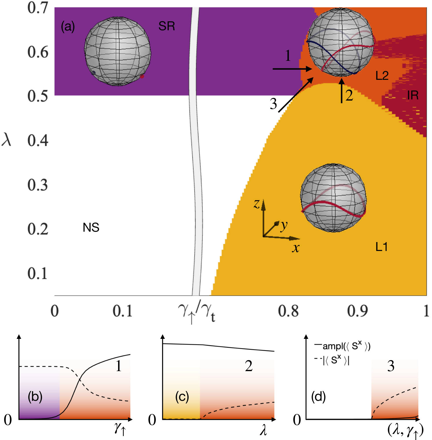
Dynamical phase diagram. By turning on $\lambda$ together with sizeable spin pumping in a weakly coupling limit ($\eta$, $\eta^{\prime}\to 0^{+}$), we generate the diagram of dynamical responses (cf. Fig. 2) in mean-field treatment, which is exact for $N\to\infty$ Bhaseen et al. 2012; Torre et al. 2013; Lang and Piazza 2016. In the Supplemental Materials sup we present the associated equations of motion and also analyze the breakdown of mean field from finite $N$ corrections.

For strong pumping ($\gamma_{\uparrow}>\gamma_{t}/2$), the spins in the ensemble $\mathcal{S}$ display long-lived oscillatory dynamics (see Bloch spheres in Fig. 2). The region L1 in Fig. 2 resembles the regular lasing Kirton and Keeling 2017 discussed above, while L2 features ’supperradiant’ oscillations. The transition from L1 to L2 occurs around values of the Dicke coupling $\sim\lambda_{c}$, with a non-vanishing time average of $\langle\mathcal{S}^{x}\rangle$ in L2. In this phase we observe persistent oscillatory dynamics reminiscent of lasing around one of the symmetry-broken states of the Dicke model. Such ’superradiant’ oscillations would not arise by directly pumping a Dicke model through the Lindblad channels in Eq. (2); they are a result of the pumping scheme of Fig. 1 conceptually borrowed from spintronics. In this regard, the dynamical phase L2 is a conceptual ’bridge’ between the quantum optics and spintronics communities which we are aiming to lay out in this work. Notice that despite the pumped subsystem experiences population inversion, the spin ensemble $\mathcal{S}$ remains in a state with negative $\langle\mathcal{S}^{z}\rangle$ in both phases L1 and L2.

We now discuss the role of symmetries in the oscillatory dynamics displayed in L1 and L2, and in the transitions between these two different regimes. For $\lambda=0$ the photon number $n$ does not oscillate. A nonzero $\lambda$ breaks the U(1) symmetry and the oscillations in $n$ can be attributed to ellipticity (i.e., different amplitudes of oscillations of $\langle\mathcal{S}\rangle$ spin components along $x$ and $y$ directions due to the presence of Dicke-like interaction term) in the spontaneous procession in absence of $\mathcal{S}^{z}$ conservation. In fact, the dynamics are instead governed by a $\mathbb{Z}_{2}$ symmetry, reflected in the observation that the oscillatory frequency of $n$ and $\langle\mathcal{S}^{z}\rangle$ is twice that of $\langle\mathcal{S}^{x}\rangle$. The transition from L1 to L2 is characterized by an increase in the time-average value of $\langle\mathcal{S}^{x}\rangle$, which can be explained by the spontaneous breaking of the $\mathbb{Z}_{2}$ symmetry upon increasing the Dicke coupling $\lambda$ [cf. Fig. 2(c)]. The transition from the SR region to the L2 region appears as a crossover in finite-time numerical data, as the damping of the oscillations of $\langle\mathcal{S}^{x}\rangle$ critically slows down upon approaching the transition point from the SR side, hence the time-averaged amplitude of the oscillations in a long but finite time windows smoothly grows, blurring the expected singular behavior at the phase boundary [cf. Fig. 2(b)] associated to the dynamical spontaneous symmetry breaking of the U(1) symmetry. Finally, in the transition from NS to L2, the absolute value of the time average of $\langle\mathcal{S}^{x}\rangle$, as well as its amplitude, build up [cf. Fig. 2(d)].

This dynamical phase diagram with competing stationary (NS, SR) and oscillatory (L1, L2, IR) phases is of particular interest to spintronics, since it emerges from the interplay of incoherent spin pumping and ellipticity. U(1) symmetry is previously taken to be an important condition in studies of spin-wave lasing Bender et al. 2012; Bender et al. 2014, though it is often broken in magnets with anisotropies. By explicitly taking this into consideration, our study suggests richer phenomena accompanying non-equilibrium phase transitions in spintronic devices. Although our model description distillates only the essential mechanisms of an actual spintronics setup, we now briefly discuss some possible implications of our results. The magnon ‘lasing’ Berger 1996 in a uniaxial magnet can converge to a steady condensate density featured by a circular precession Bender et al. 2012; Bender et al. 2014. Turning on interactions explicitly breaking the U(1) symmetry is expected to induce an ellipticity in the spontaneous precession Serga et al. 2012, accompanied by an oscillation of the condensate density due to the absence of spin conservation. This is similar to the dynamics observed in the L1 phase with $\lambda\neq 0$. In the regime where both $\mathbb{Z}_{2}$ interactions and the pumping effects are sizable, two equivalent $\mathbb{Z}_{2}$-breaking limit cycles are possible (L2 phase). During the electrical pumping, angular momentum transfers reciprocally between the magnet and metal Tserkovnyak and Bender 2014: as the itinerant electrons exert a spin torque to establish the magnon lasing, the coherent magnetic precession simultaneously pumps a spin current back into the metal Tserkovnyak et al. 2002, triggering transverse spin dynamics. Therefore, suppressing the transverse spin dynamics in the metal can be detrimental to magnon lasing, as consistent with the consequence of a fast-relaxing incoherent subsystem discussed above (large $\gamma_{t}$ limit, see SM for more details).

Polaritonic lasing. Observables in the L1 and L2 phases show signatures of upper (U) and lower (L) polaritonic modes Emary and Brandes 2003, which are symmetric (U) and anti-symmetric (L) linear superpositions of spin and photon fields, describing light-matter hybridization via the Dicke coupling $\lambda$. In order to appreciate this point, we rewrite the interaction term in (1) as $H_{int}=(\eta a+\eta^{\prime}\mathcal{S}^{-})\mathcal{T}^{+}+h.c.$, which is suggestive that pumping the $\mathcal{T}$ ensemble can excite a superposition of light and matter in the $\mathcal{S}$ system. Thus, upper or lower polaritons can be excited in the system, depending whether the two couplings have same or opposite sign, jointly with the resonance condition, $\omega^{\prime}_{z}\simeq\Omega_{U/L}$ (for related expressions, cf.  sup). The effective decay rates of the two polariton modes depend on the frequency of the incoherent subsystem $\omega_{z}^{\prime}$ and in particular, for $\eta=\eta^{\prime},$ it can be analytically estimated sup as ${\kappa}^{\textit{eff}}_{U}$$=\kappa/2-2\eta^{2}(\gamma_{\uparrow}-\gamma_{\downarrow})/\left[(\omega_{z}^{\prime}-\Omega_{U})^{2}+\gamma_{t}^{2}/4\right]$. By tuning $\omega_{z}^{\prime}$ close to $\Omega_{U}$, where

it is possible to obtain a negative effective decay rate (${\kappa}^{\textit{eff}}_{U}<0$) for $\gamma_{\uparrow}>\gamma_{\downarrow}$. The time evolution of $\langle\mathcal{S}^{z}\rangle$, $\langle\mathcal{T}^{z}\rangle$, and $n$ in this scenario are plotted in Fig. 3. The negative decay rate gives rise to dynamical instabilities in the L1 and L2 regimes, which we can exploit to employ the spin ensemble $\mathcal{T}$ as a frequency-dependent gain medium Gao et al. 2015; Lebreuilly et al. 2016; Kapit et al. 2014 (see SM for more details).

We now discuss the multi-stage dynamics [as marked by A to D in Fig. 3(b)] associated with this mechanism. We initialise the system in the SR steady state of the Dicke model with photon losses ($\lambda=0.6$ and $\kappa=0.06$) and let it evolve with parameters characteristic of the L1 phase ($\lambda=0.2$, $\gamma_{\uparrow}=0.9$). For the chosen parameters, the effective decay rate ${\kappa}^{\textit{eff}}_{L}$ (${\kappa}^{\textit{eff}}_{U}$) is positive (negative), i.e., the upper polariton becomes unstable. Immediately after the quench (A), the photon field has sizeable overlap with the upper and lower polariton modes. Since in the initial SR steady state the boson is enslaved to matter, $\langle a\rangle=-2\lambda/(\omega_{c}-i\kappa/2)\langle\mathcal{S}^{-}\rangle$, the amplitude of the lower mode is higher than the amplitude of the upper one. However, as the lower mode starts to decay and the upper one is enhanced, their amplitudes become comparable (B) and we observe beating at their two frequencies. At the stage (C) the photon number increases while the lower mode is largely suppressed. As a result, for long times (D) the oscillatory dynamics of the system is solely governed by $\Omega_{U}.$ Such circumstance cannot occur in a more conventional driven-dissipative Dicke model Kirton and Keeling 2018, since in that case both upper and lower modes would be enhanced and survive at long times.

Outlook. A natural next step could consist in studying collective spin squeezing in the lasing regime Ma et al. 2011; Pezze et al. 2018; Koppenhöfer et al. 2021, with the perspective of entanglement manipulation in spintronics platforms. This can be addressed, for instance, by simulating numerically exact dynamics at finite $N$ Shammah et al. 2018; Lerose and Pappalardi 2020.

Recent studies have shown the usefulness of non-local dissipation in generating entanglement between distant qubits in both fields of quantum optics and spintronics, by investigating spins immersed in a optical cavity Seetharam et al. 2021a; Seetharam et al. 2021b; Marino 2021 and nitrogen-vacancy qubits in proximity to a magnetic medium Zou et al. 2021. For the latter, dynamical phase transitions in the magnet controlled by electrical pumping, may provide an efficient tunability of non-local dissipation, which could be studied along the lines of this work.

Finally, we did not include here the effect of short-range spin interactions breaking permutational symmetry. This is in general a challenging task since it requires a full many-body treatment of dynamics. However, we expect that, deep inside the various phases, the dynamical phenomena discussed here will still hold in analogy with the character of other non-equilibrium phases in spin systems with competing short- and all-to-all interactions Lerose et al. 2019; Zhu et al. 2019.

Our results can be considered as a roadmap to build a novel generation of spintronics experiments inspired by quantum optics, with focus on dynamical phase transitions in heterolayers structures. Scaling up our proof of concept to more concrete platforms appears as an exciting future direction.

Acknowledgements. JM and OC are indebted to P. Kirton for enlightening discussions. OC thanks S. Kelly and R. J. Valencia Tortora for helpful comments on this work. This project has been supported by the Deutsche Forschungsgemeinschaft (DFG, German Research Foundation) – Project-ID 429529648 – TRR 306 QuCoLiMa (”Quantum Cooperativity of Light and Matter”), by the Dynamics and Topology Centre funded by the State of Rhineland Palatinate, and in part by the National Science Foundation under Grant No. NSF PHY-1748958 (KITP program ’Non-Equilibrium Universality: From Classical to Quantum and Back’). J.M. and O.C. acknowledge support by the Dynamics and Topology Centre funded by the State of Rhineland Palatinate. A.L. acknowledges support by the Swiss National Science Foundation. S.Z. and Y.T. are supported by the U.S. Department of Energy, Office of Basic Energy Sciences under Grant No. DE-SC0012190. The Alexander von Humboldt Foundation is acknowledged for supporting YT’s stay at Mainz, where this work was initiated. I. C. acknowledges financial support from the H2020-FETFLAG-2018-2020 project ”PhoQuS” (n.820392), and from the Provincia Autonoma di Trento.

References

- Carusotto and Ciuti (2013) I. Carusotto and C. Ciuti, Quantum fluids of light, Rev. Mod. Phys. 85, 299 (2013).
- Stitely et al. (2020) K. C. Stitely, A. Giraldo, B. Krauskopf, and S. Parkins, Nonlinear semiclassical dynamics of the unbalanced, open dicke model, Phys. Rev. Research 2, 033131 (2020).
- Ritsch et al. (2013) H. Ritsch, P. Domokos, F. Brennecke, and T. Esslinger, Cold atoms in cavity–generated dynamical optical potentials, Rev. Mod. Phys. 85, 553 (2013).
- Houck et al. (2012) A. A. Houck, H. E. Türeci, and J. Koch, On-chip quantum simulation with superconducting circuits, Nat. Phys. 8, 292 (2012).
- Kirilyuk et al. (2010) A. Kirilyuk, A. V. Kimel, and T. Rasing, Ultrafast optical manipulation of magnetic order, Rev. Mod. Phys. 82, 2731 (2010).
- Kessler et al. (2012) E. M. Kessler, G. Giedke, A. Imamoglu, S. F. Yelin, M. D. Lukin, and J. I. Cirac, Dissipative phase transition in a central spin system, Phys. Rev. A 86, 012116 (2012).
- Hauser (1969) J. J. Hauser, Magnetic proximity effect, Phys. Rev. 187, 580 (1969).
- Saitoh et al. (2006) E. Saitoh, M. Ueda, H. Miyajima, and G. Tatara, Conversion of spin current into charge current at room temperature: Inverse spin–Hall effect, Appl. Phys. Lett. 88, 182509 (2006).
- Uchida et al. (2010) K. Uchida, J. Xiao, H. Adachi, J. Ohe, S. Takahashi, J. Ieda, T. Ota, Y. Kajiwara, H. Umezawa, H. Kawai, G. E. Bauer, S. Maekawa, and E. Saitoh, Spin Seebeck insulator, Nat. Mater. 9, 894 (2010).
- Kajiwara et al. (2010) Y. Kajiwara, K. Harii, S. Takahashi, J. Ohe, K. Uchida, M. Mizuguchi, H. Umezawa, H. Kawai, K. Ando, K. Takanashi, et al., Transmission of electrical signals by spin–wave interconversion in a magnetic insulator, Nature 464, 262 (2010).
- Czeschka et al. (2011) F. D. Czeschka, L. Dreher, M. S. Brandt, M. Weiler, M. Althammer, I.-M. Imort, G. Reiss, A. Thomas, W. Schoch, W. Limmer, H. Huebl, R. Gross, and S. T. B. Goennenwein, Scaling behavior of the spin pumping effect in ferromagnet–platinum bilayers, Phys. Rev. Lett. 107 (2011).
- Huang et al. (2012) S. Y. Huang, X. Fan, D. Qu, Y. P. Chen, W. G. Wang, J. Wu, T. Y. Chen, J. Q. Xiao, and C. L. Chien, Transport magnetic proximity effects in platinum, Phys. Rev. Lett. 109, 107204 (2012).
- Althammer et al. (2013) M. Althammer, S. Meyer, H. Nakayama, M. Schreier, S. Altmannshofer, M. Weiler, H. Huebl, S. Geprägs, M. Opel, R. Gross, D. Meier, C. Klewe, T. Kuschel, J.-M. Schmalhorst, G. Reiss, L. Shen, A. Gupta, Y.-T. Chen, G. E. W. Bauer, E. Saitoh, and S. T. B. Goennenwein, Quantitative study of the spin Hall magnetoresistance in ferromagnetic insulator/normal metal hybrids, Phys. Rev. B 87, 224401 (2013).
- Lin et al. (2013) T. Lin, C. Tang, and J. Shi, Induced magneto–transport properties at palladium/yttrium iron garnet interface, Appl. Phys. Lett. 103, 132407 (2013).
- Hahn et al. (2013) C. Hahn, G. de Loubens, O. Klein, M. Viret, V. V. Naletov, and J. Ben Youssef, Comparative measurements of inverse spin Hall effects and magnetoresistance in YIG/Pt and YIG/Ta, Phys. Rev. B 87, 174417 (2013).
- Kittel and Fong (1963) C. Kittel and C. Y. Fong, Quantum theory of solids, Vol. 5 (Wiley New York, 1963).
- Dyakonov and Perel (1971) M. I. Dyakonov and V. Perel, Current–induced spin orientation of electrons in semiconductors, Phys. Lett. A 35, 459 (1971).
- Demokritov et al. (2006) S. O. Demokritov, V. E. Demidov, O. Dzyapko, G. A. Melkov, A. A. Serga, B. Hillebrands, and A. N. Slavin, Bose–Einstein condensation of quasi–equilibrium magnons at room temperature under pumping, Nature 443, 430 (2006).
- Demidov et al. (2008) V. E. Demidov, O. Dzyapko, S. O. Demokritov, G. A. Melkov, and A. N. Slavin, Observation of spontaneous coherence in Bose–Einstein condensate of magnons, Phys. Rev. Lett. 100, 047205 (2008).
- Duine et al. (2017) R. A. Duine, A. Brataas, S. A. Bender, and Y. Tserkovnyak, Spintronics and magnon Bose–Einstein condensation, in Universal Themes of Bose–Einstein Condensation, edited by N. P. Proukakis, D. W. Snoke, and P. B. Littlewood (Cambridge University Press, 2017) p. 505–524.
- Giamarchi et al. (2008) T. Giamarchi, C. Rüegg, and O. Tchernyshyov, Bose–Einstein condensation in magnetic insulators, Nat. Phys. 4, 198 (2008).
- Berger (1996) L. Berger, Emission of spin waves by a magnetic multilayer traversed by a current, Phys. Rev. B 54, 9353 (1996).
- Bunkov and Volovik (2007) Y. M. Bunkov and G. E. Volovik, Magnon condensation into a ball in , Phys. Rev. Lett. 98, 265302 (2007).
- Bunkov and Volovik (2008) Y. M. Bunkov and G. E. Volovik, Bose–Einstein condensation of magnons in superfluid 3He, Low Temp. Phys. 150, 135 (2008).
- Bender et al. (2012) S. A. Bender, R. A. Duine, and Y. Tserkovnyak, Electronic pumping of quasiequilibrium Bose–Einstein–condensed magnons, Phys. Rev. Lett. 108, 246601 (2012).
- Bender et al. (2014) S. A. Bender, R. A. Duine, A. Brataas, and Y. Tserkovnyak, Dynamic phase diagram of dc–pumped magnon condensates, Phys. Rev. B 90, 094409 (2014).
- Fjærbu et al. (2017) E. L. Fjærbu, N. Rohling, and A. Brataas, Electrically driven Bose–Einstein condensation of magnons in antiferromagnets, Phys. Rev. B 95, 144408 (2017).
- Takei (2019) S. Takei, Spin transport in an electrically driven magnon gas near Bose-Einstein condensation: Hartree–Fock–Keldysh theory, Phys. Rev. B 100, 134440 (2019).
- Wimmer et al. (2019) T. Wimmer, M. Althammer, L. Liensberger, N. Vlietstra, S. Geprägs, M. Weiler, R. Gross, and H. Huebl, Spin transport in a magnetic insulator with zero effective damping, Phys. Rev. Lett. 123, 257201 (2019).
- Hurd (2012) C. Hurd, The Hall effect in metals and alloys (Springer Science & Business Media, 2012).
- Hirsch (1999) J. E. Hirsch, Spin Hall effect, Phys. Rev. Lett. 83, 1834 (1999).
- Kato et al. (2004) Y. K. Kato, R. C. Myers, A. C. Gossard, and D. D. Awschalom, Observation of the spin Hall effect in semiconductors, Science 306, 1910 (2004).
- Sih et al. (2005) V. Sih, R. Myers, Y. Kato, W. Lau, A. Gossard, and D. Awschalom, Spatial imaging of the spin Hall effect and current–induced polarization in two–dimensional electron gases, Nat. Phys. 1, 31 (2005).
- Wunderlich et al. (2005) J. Wunderlich, B. Kaestner, J. Sinova, and T. Jungwirth, Experimental observation of the spin–Hall effect in a two–dimensional spin–orbit coupled semiconductor system, Phys. Rev. Lett. 94, 047204 (2005).
- Valenzuela and Tinkham (2006) S. O. Valenzuela and M. Tinkham, Direct electronic measurement of the spin Hall effect, Nature 442, 176 (2006).
- Slonczewski (1996) J. C. Slonczewski, Current-driven excitation of magnetic multilayers, J. Magn. Magn. Mater. 159, L1 (1996).
- Ralph and Stiles (2008) D. C. Ralph and M. D. Stiles, Spin transfer torques, J. Magn. Magn. Mater. 320, 1190 (2008).
- Tserkovnyak and Bender (2014) Y. Tserkovnyak and S. A. Bender, Spin Hall phenomenology of magnetic dynamics, Phys. Rev. B 90, 014428 (2014).
- Flebus et al. (2016) B. Flebus, S. A. Bender, Y. Tserkovnyak, and R. A. Duine, Two-fluid theory for spin superfluidity in magnetic insulators, Phys. Rev. Lett. 116, 117201 (2016).
- Kirton et al. (2019) P. Kirton, M. M. Roses, J. Keeling, and E. G. Dalla Torre, Introduction to the Dicke model: From equilibrium to nonequilibrium, and vice versa, Advanced Quantum Technologies 2, 1800043 (2019).
- Emary and Brandes (2003) C. Emary and T. Brandes, Chaos and the quantum phase transition in the Dicke model, Phys. Rev. E 67, 066203 (2003).
- Bhaseen et al. (2012) M. J. Bhaseen, J. Mayoh, B. D. Simons, and J. Keeling, Dynamics of nonequilibrium Dicke models, Phys. Rev. A 85, 013817 (2012).
- Keeling et al. (2010) J. Keeling, M. J. Bhaseen, and B. D. Simons, Collective dynamics of Bose–Einstein condensates in optical cavities, Phys. Rev. Lett. 105, 043001 (2010).
- Reiter et al. (2020) F. Reiter, T. L. Nguyen, J. P. Home, and S. F. Yelin, Cooperative breakdown of the oscillator blockade in the Dicke model, Phys. Rev. Lett. 125, 233602 (2020).
- Breuer et al. (2002) H. P. Breuer, F. Petruccione, et al., The theory of open quantum systems (Oxford University Press on Demand, 2002).
- Mayergoyz et al. (2009) I. D. Mayergoyz, G. Bertotti, and C. Serpico, Nonlinear magnetization dynamics in nanosystems (Elsevier, 2009).
- Gilbert (2004) T. L. Gilbert, A phenomenological theory of damping in ferromagnetic materials, IEEE Trans. Magn. 40, 3443 (2004).
- Bode et al. (2011) N. Bode, S. V. Kusminskiy, R. Egger, and F. von Oppen, Scattering theory of current–induced forces in mesoscopic systems, Phys. Rev. Lett. 107, 036804 (2011).
- (49) See Supplemental Material for MF equations of motion, Gilbert damping, lasing instabilities, polariton analysis and cumulants expansion.
- Dicke (1954) R. H. Dicke, Coherence in spontaneous radiation processes, Phys. Rev. 93, 99 (1954).
- Kirton and Keeling (2018) P. Kirton and J. Keeling, Superradiant and lasing states in driven–dissipative Dicke models, New J. Phys. 20, 015009 (2018).
- Kirton and Keeling (2017) P. Kirton and J. Keeling, Suppressing and restoring the Dicke superradiance transition by dephasing and decay, Phys. Rev. Lett. 118, 123602 (2017).
- Tieri et al. (2017) D. Tieri, M. Xu, D. Meiser, J. Cooper, and M. Holland, Theory of the crossover from lasing to steady state superradiance, arXiv preprint arXiv:1702.04830 (2017).
- Kopylov et al. (2015) W. Kopylov, M. Radonjić, T. Brandes, A. Balaž, and A. Pelster, Dissipative two–mode Tavis–Cummings model with time–delayed feedback control, Phys. Rev. A 92, 063832 (2015).
- Torre et al. (2013) E. G. D. Torre, S. Diehl, M. D. Lukin, S. Sachdev, and P. Strack, Keldysh approach for nonequilibrium phase transitions in quantum optics: Beyond the Dicke model in optical cavities, Phys. Rev. A 87, 023831 (2013).
- Lang and Piazza (2016) J. Lang and F. Piazza, Critical relaxation with overdamped quasiparticles in open quantum systems, Phys. Rev. A 94, 033628 (2016).
- Serga et al. (2012) A. A. Serga, C. W. Sandweg, V. I. Vasyuchka, M. B. Jungfleisch, B. Hillebrands, A. Kreisel, P. Kopietz, and M. P. Kostylev, Brillouin light scattering spectroscopy of parametrically excited dipole–exchange magnons, Phys. Rev. B 86, 134403 (2012).
- Tserkovnyak et al. (2002) Y. Tserkovnyak, A. Brataas, and G. E. W. Bauer, Enhanced Gilbert damping in thin ferromagnetic films, Phys. Rev. Lett. 88, 117601 (2002).
- Gao et al. (2015) T. Gao, C. Antón, T. C. H. Liew, M. Martín, Z. Hatzopoulos, L. Viña, P. Eldridge, and P. Savvidis, Spin selective filtering of polariton condensate flow, Appl. Phys. Lett. 107, 011106 (2015).
- Lebreuilly et al. (2016) J. Lebreuilly, M. Wouters, and I. Carusotto, Towards strongly correlated photons in arrays of dissipative nonlinear cavities under a frequency–dependent incoherent pumping, Comptes Rendus Physique 17, 836 (2016).
- Kapit et al. (2014) E. Kapit, M. Hafezi, and S. H. Simon, Induced self-stabilization in fractional quantum Hall states of light, Phys. Rev. X 4, 031039 (2014).
- Ma et al. (2011) J. Ma, X. Wang, C. P. Sun, and F. Nori, Quantum spin squeezing, Phys. Rep. 509, 89 (2011).
- Pezze et al. (2018) L. Pezze, A. Smerzi, M. K. Oberthaler, R. Schmied, and P. Treutlein, Quantum metrology with nonclassical states of atomic ensembles, Rev. Mod. Phys. 90, 035005 (2018).
- Koppenhöfer et al. (2021) M. Koppenhöfer, P. Groszkowski, H. K. Lau, and A. A. Clerk, Dissipative superradiant spin amplifier for enhanced quantum sensing (2021), arXiv:2111.15647 [quant-ph] .
- Shammah et al. (2018) N. Shammah, S. Ahmed, N. Lambert, S. De Liberato, and F. Nori, Open quantum systems with local and collective incoherent processes: Efficient numerical simulations using permutational invariance, Phys. Rev. A 98, 063815 (2018).
- Lerose and Pappalardi (2020) A. Lerose and S. Pappalardi, Bridging entanglement dynamics and chaos in semiclassical systems, Phys. Rev. A 102, 032404 (2020).
- Seetharam et al. (2021a) K. Seetharam, A. Lerose, R. Fazio, and J. Marino, Correlation engineering via non–local dissipation, arXiv:2101.06445 (2021a).
- Seetharam et al. (2021b) K. Seetharam, A. Lerose, R. Fazio, and J. Marino, Dynamical scaling of correlations generated by short– and long–range dissipation (2021b), arXiv:2110.09547 [cond-mat.quant-gas] .
- Marino (2021) J. Marino, Universality class of Ising critical states with long–range losses (2021), arXiv:2108.12422 [cond-mat.stat-mech] .
- Zou et al. (2021) J. Zou, S. Zhang, and Y. Tserkovnyak, Bell–state generation for spin qubits via dissipative coupling, arXiv:2108.07365 (2021).
- Lerose et al. (2019) A. Lerose, B. Žunkovič, J. Marino, A. Gambassi, and A. Silva, Impact of nonequilibrium fluctuations on prethermal dynamical phase transitions in long-range interacting spin chains, Phys. Rev. B 99, 045128 (2019).
- Zhu et al. (2019) B. Zhu, J. Marino, N. Y. Yao, M. D. Lukin, and E. A. Demler, Dicke time crystals in driven–dissipative quantum many–body systems, New J. Phys. 21, 073028 (2019).
- Landau and Lifshitz (1992) L. Landau and E. Lifshitz, On the theory of the dispersion of magnetic permeability in ferromagnetic bodies, in Perspectives in Theoretical Physics (Elsevier, 1992) pp. 51–65.
- Gilbert (1955) T. Gilbert, A lagrangian formulation of the gyromagnetic equation of the magnetization field, Phys. Rev. 100, 1243 (1955).
- Holstein and Primakoff (1940) T. Holstein and H. Primakoff, Field dependence of the intrinsic domain magnetization of a ferromagnet, Phys. Rev. 58, 1098 (1940).
- Agarwal et al. (1997) G. S. Agarwal, R. R. Puri, and R. P. Singh, Atomic Schrödinger cat states, Phys. Rev. A 56, 2249 (1997).
- Xu (2016) M. Xu, Theory of steady–state superradiance, Ph.D. thesis, University of Colorado at Boulder (2016).
- Norcia et al. (2018) M. A. Norcia, R. J. Lewis-Swan, J. R. Cline, B. Zhu, A. M. Rey, and J. K. Thompson, Cavity–mediated collective spin–exchange interactions in a strontium superradiant laser, Science 361, 259 (2018).
- Haken (1975) H. Haken, Cooperative phenomena in systems far from thermal equilibrium and in nonphysical systems, Rev. Mod. Phys. 47, 67 (1975).
- Haken (1984) H. Haken, The semiclassical approach and its applications, in Laser Theory (Springer, 1984) pp. 173–248.
- Negele and Orland (2018) J. W. Negele and H. Orland, Quantum many–particle systems (CRC Press, 2018).
- Huang (2009) K. Huang, Introduction to statistical physics (Chapman and Hall/CRC, 2009).
- Lewenstein and You (1996) M. Lewenstein and L. You, Quantum phase diffusion of a Bose–Einstein condensate, Phys. Rev. Lett. 77, 3489 (1996).
- Amelio and Carusotto (2020) I. Amelio and I. Carusotto, Theory of the coherence of topological lasers, Phys. Rev. X 10, 041060 (2020).
Appendix A Stability analysis
The mean-field equations of motion used to derive the phase diagram in Fig. 2(a) read