Stochastic and deterministic dynamics in networks with excitable nodes

The collective behavior of networks comprised of excitable nodes has found applications in many systems ranging from avalanches of neuronal bursting in the mammalian cortex Beggs and Plenz 2003; Petermann et al. 2009 and neuroscience as a whole Gerstner et al. 2014; Stewart and Plenz 2008; Shew et al. 2009; Larremore et al. 2012; De Arcangelis et al. 2006; de Arcangelis and Herrmann 2010 to epidemiology Miller 2009; Allard et al. 2009 and social systems Miller 2009; Kinouchi and Copelli 2006, in all of which the effect of stochasticity in believed to be crucial. This stochasticity in the dynamics of the excitable nodes is understood in two levels: models with single excitable agents with stochastic external stimuli, and coarse-grained models where each node refers to many agents whose collective response to the stimuli is stochastic. This stochasticity was proven to be responsible for various behaviors of the system, like a second-order non-equilibrium phase transition separating the absorbing state from the super-critical state Larremore et al. 2011a; Larremore et al. 2012, bifurcation and oscillatory behavior Moosavi et al. 2017; Najafi and Rahimi-Majd 2019, and a critical transition line with varying exponents Rahimi-Majd et al. 2021. Among a long list of various collective modes of the system, arguably criticality is believed to be the most important state affecting the system functioning, including optimal dynamical range Larremore et al. 2011a; Larremore et al. 2011b; Kinouchi and Copelli 2006; Shew et al. 2009, synaptic learning de Arcangelis and Herrmann 2010 and optimal information processing Kinouchi and Copelli 2006. This state can be achieved in a self-organized fashion (as expected in the brain) which is a source of many theoretical studies based on the network plasticity (brain plasticity in De Arcangelis et al. 2006), and experimental studies, e.g., by tuning the ratios of excitation to inhibition for cortex slice cultures grown on planar microelectrode arrays Shew et al. 2009. The basic assumption in the theoretical studies is the linearity of the master equations with respect to excitation probability of single node $p_{t}$ Larremore et al. 2011a. This assumption is however violated for systems with leading higher order terms with non-linear expansion around the transition point (see the following). The deterministic dynamics with threshold is an extreme example which applies for, e.g., sandpile-like dynamics on complex networks Najafi 2014; Najafi et al. 2020; Najafi and Dashti-Naserabadi 2018. In this paper we uncover a rich phase space by introducing and analyzing an interpolation parameter $\beta$, which interpolates between stochastic and deterministic dynamics.

Working with the (stochastic) Kinouchi-Copelli (KC) model Kinouchi and Copelli 2006, it was shown by Larremore et al. Larremore et al. 2011a that for networks with stochastic dynamics the largest eigenvalue $\lambda$ of the adjacency matrix $A$ (approximated to be $\lambda=\sigma\left\langle k\right\rangle$ for the Erdős-Rényi network Restrepo et al. 2007 where $\sigma$ is the maximum weight of links, and $\left\langle k\right\rangle$ is the average of the node degree) and its associated eigenvector play a prominent role in determining the functional form and consequently the status of the system, i.e., for $\lambda<\lambda_{c}\equiv 1$ the system is in the absorbing state where no node is excited, while for $\lambda>\lambda_{c}$ the activity of the system saturates eventually to a state where a macroscopic fraction of the nodes are “on”. The key strategy in this work, that was followed later by many authors for other different dynamical models Larremore et al. 2011b; Larremore et al. 2012; Moosavi et al. 2017 was linearizing the governing master equations and also the system’s response function $F\equiv\left\langle f\right\rangle_{t}$ (with $\left\langle\right\rangle_{t}$ denoting an average over time and $f$ the fraction of excited nodes) with respect to the nodes’ firing probability $p^{t}$ being small near the transition point $\lambda_{c}$. This strategy was proven to be general enough to give the properties of the system in the vicinity of the transition point given that the system response $F$ linearly vanishes when the external stimuli approaches zero Brochini et al. 2016, which we call linear stochasticity. The inclusion of a refractory period causes additionally another transition point ($\lambda_{b}\equiv 2$) at which the system undergoes a bifurcation Moosavi et al. 2017. Therefore, the phase diagram of these systems is given by

Many additional effects, like the impact of inhibitory nodes Larremore et al. 2014, the effect of short-range sensory nodes (changing continuously $\lambda_{c}$ and $\lambda_{b}$) Rahimi-Majd et al. 2021, and retardation effects Najafi and Rahimi-Majd 2019 were based on this analysis and the inspection of the activity-dependent branching ratio $b(M)$ Martin et al. 2010.

Here we show how the assumption of linear stochasticity can be relaxed (details in Appendix A). The network in the KC model Kinouchi and Copelli 2006 is comprised of excitable nodes where each node $i$ can be in one of active or quiescent states, so that $x_{i}(t)=0\;(1)$ characterizes the non-firing (firing) state, and $p_{i}^{t}=P(x_{i}(t)=1)$. Analytical treatments of this model usually assume locally tree-like networks which are defined as those networks where for $t$ not too large there is maximally one path of length $t$ for any pair $j$ and $k$. Besides the stochasticity in the dynamics, the basic assumption in Larremore et al. 2011a is that one excited node is enough to excite a neighboring node given that the later is not in the refractory period. Based on this, a master equation (Eq. 1 in SM) is developed and linearized (as well as $F$) with respect to $p^{t}$ and the input stimuli $x$ in the vicinity of the critical point $\lambda=\lambda_{c}$ Larremore et al. 2011a; Larremore et al. 2012; Larremore et al. 2011b. The violation of this linearity changes the thermodynamic properties of the system. Consider for example a locally tree network with $N$ excitable nodes in which $\alpha$ excited nodes are required for exciting a destination node. Then, one can show that in terms of the KC model Kinouchi and Copelli 2006 $F$ vanishes with the $\alpha$th power of $x$ in the limit $x\rightarrow 0$, and in the leading order (see Eq. 5 in SM)

where $A_{ij}$ is the adjacency matrix of the network, i.e. $A_{ij}=w_{ij}$ if there is connection between $i$ and $j$ and zero otherwise, and $w_{ij}$ is a weight function. In an extreme limit $F$ is zero below a threshold and becomes non-zero abruptly beyond this threshold, which is a deterministic dynamics. Here we address this problem in a general setup using a parameter $\beta$ which besides making the dynamics non-linear, interpolates between linear stochastic ($\beta=0$) and nonlinear deterministic ($\beta=\infty$) dynamics, resulting in a rich phase diagram. In addition to studying the effect of a nonlinear transfer function, we explore the effect of a finite network. Theoretical analyses are usually carried out in the $N\to\infty$ limit, and initial conditions are chosen by implicitly assuming that a constant fraction of the nodes are initially excited. Here we also consider the case where $N$ is large but finite, and the system is started with only one excited node. We show that the effective phase diagram for this case is qualitatively different from the phase diagram obtained when a constant nonzero fraction of the $N\to\infty$ nodes is excited.

Our model consists of $N$ excitable nodes on a random directed graph where each pair of nodes are connected with probability $q$, resulting in an average (equal) node in- and out-degree $\langle k\rangle=q(N-1)$. The connection weights $w_{i,j}$ are randomly distributed in the interval $[0,2\sigma]$, where $\sigma$ is a tuning parameter. The leading control parameter is the largest eigenvalue of $A_{ij}$, which is $\lambda\approx\sigma qN$ in our case (see Eq. 1). The dynamics is like the KC model presented above, taking into account that some nodes are in the refractory period, i.e., the node cannot be excited immediately after being excited in the previous step. The probability that a node $i$ spikes at time $t+1$ is Larremore et al. 2014

where $\delta_{x_{i}(t),0}$ is unity if $x_{i}(t)=0$ and zero otherwise, i.e., it is the effect of the refractory period of one time step. $h_{\beta}$ is a dynamical transfer function which gives the probability that a node becomes active based on the total input, which is chosen to be $h_{\beta}(x)=G(h_{0}(x,\beta))$ where $G(x)$ is $x$ when $0\leq x\leq 1$, $1$ if $x>1$, and $0$ if $x<0$, and $h_{0}(x,\beta)$ is

The function $h_{\beta}(x)$ (Fig. 1 in SM) interpolates between linear stochastic ($\beta=0$ where the probability of spike increases linearly with the input potential Larremore et al. 2014; Moosavi et al. 2017) and a step-like function of input which shows a deterministic dynamics ($\beta\rightarrow\infty$ where a node is excited only when the input potential exceeds a threshold, arbitrarily set to unity). When $\beta\rightarrow 0$, it was shown that in the continuum limit for large network sizes the model reduces to Wilson-Cowan equations Wilson and Cowan 1972 when both the inhibitory and excitatory nodes (neurons) are present Benayoun et al. 2010. There it was shown that one way to reach criticality is adjusting the inhibitory and excitatory strengths in the system, which serve as a mechanism for neuronal avalanches Benayoun et al. 2010.
As discussed above, in order to highlight the interplay between the initial conditions for the dynamics and finite-size effects in the system, two initial states (at $t=0$) are considered here: ($\mathbb{I}$) only one node is excited, and ($\mathbb{II}$) a macroscopic fraction of nodes (here $10\%$) are initially excited. For the case ($\mathbb{I}$) the transition between absorbing and supercritical phases is shown to be continuous for $\beta=0$ and is of first order for large $\beta$s, for which hysteretic behavior is observed. Our analytical and numerical results show that in the thermodynamic limit for $\beta>0$, the only dominant phase for the case ($\mathbb{I}$) is the absorbing state, i.e. initial conditions with $x^{0}$ invariable are attracted to $x^{*}=0$. For the case ($\mathbb{II}$) the transition lines are $\beta$-dependent in the thermodynamic limit. In particular, the bifurcation line jumps to $\lambda_{b}=4$ for non-zero $\beta$’s. Based on a mean field (MF) analysis we propose a one-dimensional map (by reducing Eq. 3) that gives us the behavior of the system in the thermodynamic limit of both cases, and enables us to treat the problem analytically. The MF theory is presented in the SM, where we developed MF theory for both cases separately, which is based on the analysis of the local activity defined as $s_{t}\equiv\frac{1}{N}\sum_{i=1}^{N}x_{i}(t)$. Here we briefly summarize the approach for both cases. For case ($\mathbb{I}$) the main question is to determine when the excitation of a single node will lead to the absorbing state $s^{*}=0$. One can easily show that when one node is initially excited, $x_{n}(0)=\delta_{n,i}$, the expected network activity at $t=1$ is given by

where $\mathbb{E}\left[s_{t}\right]$ is the ensemble average of $s_{t}$. For an ER network with weight $w\in[0,2\sigma]$ one obtains (see SM)

One then can find the transition point by setting $b=1$: for $b<1$ activity dies (on average) and approaches $s^{*}=0$, and for $b>1$ it becomes self-sustained. By expanding $h_{\beta}$ for the limit $N\rightarrow\infty$, one finds (see SM) that $\lambda_{c}\propto N^{\frac{\beta}{\beta+1}}$. More generally, the equation $b=1$ gives the parameter curve separating $s^{t}\to 0$ or $s^{t}\to s_{2}>0$.
For case ($\mathbb{II}$), by assuming statistical independence of $\delta_{x_{i}^{t},0}$ and $h_{\beta}\left(\sum_{j=1}^{N}A_{ij}x_{j}(t)\right)$ we have

where $\mathbb{E}\left[s_{t+1}\right]$ is the ensemble average of $s_{t+1}$. Now we use the fact that $\left\langle\delta_{x_{i}^{t},0}\right\rangle=1-s_{t}$. Furthermore, for an Erdős-Rényi network with large mean degree the distribution of the random variable $\sum_{m=1}^{N}A_{nm}x_{m}^{t}$ is narrow about its mean $\lambda s_{t}$, so we approximate $\left\langle h_{\beta}\left(\sum_{j=1}^{N}A_{ij}x_{j}(t)\right)\right\rangle\simeq h_{\beta}\left(\lambda s_{t}\right)$, so that

By analyzing the dynamics of the one-dimensional map $s_{t+1}=(1-s_{t})h_{\beta}(\lambda s_{t})$ we are able to understand the observed behavior in case ($\mathbb{II}$).

For the simulations we considered $\frac{N}{10^{3}}=2.5,5,10,22$ and $40$, for both ($\mathbb{I}$) and ($\mathbb{II}$) initial states ($x_{i}=0,1$ for quiescent and excited nodes respectively where $i$ is randomly chosen). $10^{6}$ samples were generated for each $\lambda$ and $\beta$ and $N$, over which the ensemble averages were taken. Let us consider $s^{*}$ as the fixed point of the dynamics, which is defined as $s^{*}\equiv\lim_{t\rightarrow\infty}\left\langle s_{t}\right\rangle_{t}$, so that $s^{*}=0$ for the absorbing state (subcritical regime), and is non-zero for extended critical regime. In the oscillatory phase $s$ oscillates between two non-zero limits. The probability distribution function (PDF) of $s^{*}$ for case ($\mathbb{I}$) is shown in Fig. 1 in terms of $\beta$ which shows a bimodal structure, i.e. there are two peaks at $s^{*}_{1}=0$ and $s^{*}_{2}>0$. For very small $\lambda$ values the second peak is absent and there is only one peak at $s^{*}=0$, showing that the system is in the absorbing state regime. When we increase $\lambda$ the second peak $s^{*}_{2}$ is born for the first time in a point which we show by $\lambda^{(1)}_{c}(\beta)$. As $\lambda$ is increased further the position of the first peak is fixed, while the second peak moves to the right, and at the same time the height of the first (second) peak decreases (increases), and eventually the first peak dies at a point that we call $\lambda^{(2)}_{c}(\beta)$. This reveals that the system exhibits a discontinuity at the point where the second peak is born ($\lambda^{(1)}_{c}(\beta)$) using of which we define a gap parameter as $\Delta(\beta)\equiv s^{*}_{2}-s^{*}_{1}$. As is shown in the inset of Fig. 1, $\Delta(\beta)$ is saturated in large enough $\beta$s, and also $\lim_{\beta\rightarrow 0}\Delta=0$, i.e. the gap closes at $\beta=0$. The same behaviors are observed (not shown here) for the case ($\mathbb{II}$), with smaller gap values. The presence of two peaks with a gap in between is a signature of first order transition, while the zero gap in $\beta=0$ suggests similarities with the second order transition as is well-established in the literature.

We investigate here the activity-dependent branching ratio defined as $b(S)\equiv\mathbb{E}\left[\frac{s_{t+1}}{S}|s_{t}=S\right]$ to reveal the structure of the model, where $\mathbb{E}[A|B]$ represents ensemble average of $A$ conditioned on $B$ Martin et al. 2010. The fixed points are identified by the relation $b(s^{*})=1$, so that the continuous transition points are identified by a monotonically decreasing $b(S)$ with the condition $\lim_{S\rightarrow 0}b(S)=1$. This function (computed numerically) is shown in Fig. 2 for the case $\mathbb{I}$ for $\beta=0.3$, $N=10000$ and $\lambda=2.15$ showing two stable fixed points $s^{*}=0$ and $s^{*}\simeq 0.4608$ and one unstable fixed point $s^{*}_{\text{unstable}}\simeq 0.013$, which is consistent with the lower graph where the new peak starts to form for the first time. For $\beta=0$ at $\lambda=1$, $b(S)$ is a monotonically decreasing function of $S$ with the property $\lim_{S\rightarrow 0}b(S)=1$ as expected Larremore et al. 2014; Moosavi et al. 2017; Najafi and Rahimi-Majd 2019. As a standard approach for bimodal PDFs Xue et al. 2020, we divide the data at the valley point between $s^{*}_{1}$ and $s^{*}_{2}$ (with PDFs represented by $P_{1}(s^{*})$ and $P_{2}(s^{*})$ respectively), and average to find two $\left\langle s^{*}\right\rangle_{i}$, $i=1,2$ for two branches (this enables us find the structure of the transition, otherwise a structure like $\beta=0$ case is obtained, see Fig. 3 in the SM). The results are shown in Fig. 3a (for the case $\mathbb{I}$) and 3b (for the case $\mathbb{II}$). In these graphs the upper branch (which is calculated with respect to $P_{2}(s^{*})$) is born for the first time at $(\lambda^{(1)}_{c}(\beta),\Delta(\beta))$ as explained above, and the lower branch (which is calculated with respect to $P_{1}(s^{*})$) dies at the point $(\lambda_{c}^{(2)}(\beta),0)$. As $\lambda$ increases further, the graph passes a bifurcation point $\lambda_{b}(\beta)$ beyond which the upper branch splits into (and oscillates between) two branches, the distance between which increases by increasing $\lambda$ (first observed by Moosavi et. al. Moosavi et al. 2017). The bifurcation points are identified using the Kurthosis analysis, which for the transition point deviates from the Gaussian distribution Rahimi-Majd et al. 2021, see Fig. 5 in the SM. From this behavior shown in Fig. 3 one observes a hysteresis behavior, i.e., the loops that are extended from $\lambda^{(1)}_{c}$ to $\lambda^{(2)}_{c}$ between two branches, shown for four $\beta$ values for both $\mathbb{I}$ and $\mathbb{II}$ cases (for more graphs see SM). The range in which the hysteresis effect is observed is much larger and much more $N$-dependent for the case $\mathbb{I}$ with respect to $\mathbb{II}$. The survival of the lower branch for the case $\mathbb{I}$ (much more than the case $\mathbb{II}$) and consequently a higher hysteresis range is expected since the dynamic starts from one excited node for which the probability of turning off of the whole network is higher. Observe that as $\beta$ increases the hysteresis effect magnifies and $\lambda_{c}^{(1,2)}$ grow with $\beta$ and $N$. The MF prediction (from iteration of the map $s_{t+1}=(1-s_{t})h_{\beta}(\lambda s_{t})$) is also shown in Fig. 3b with a bold continuous line to which the graph approaches asymptotically as $N\rightarrow\infty$. This figure shows intermittent oscillatory regime, which is consistent with MF as well as the kurtosis analysis (SM).

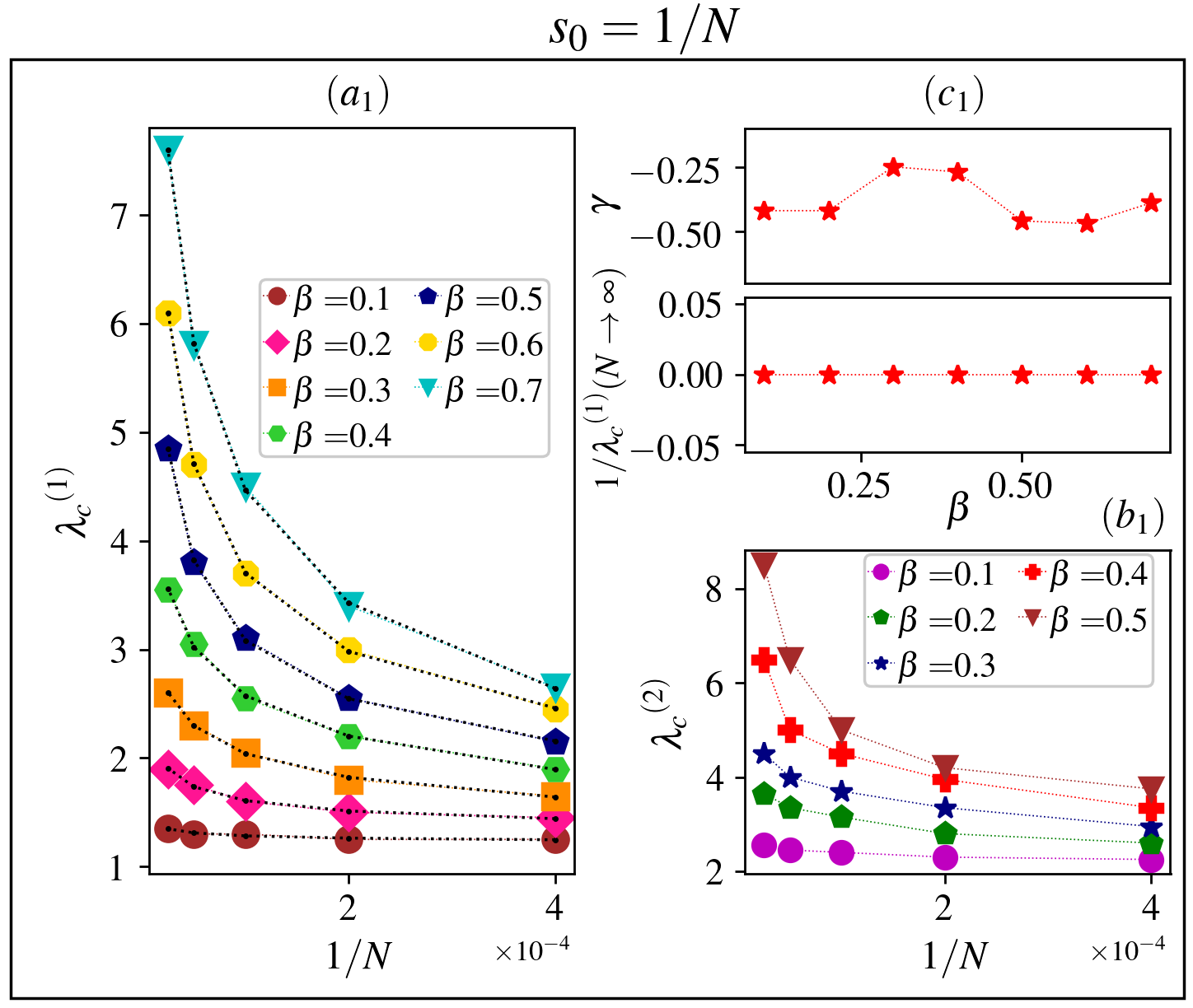
For obtaining the behavior of the model in the thermodynamic limit, we traced that behavior of the transition points for various $N$s for both $\mathbb{I}$ and $\mathbb{II}$ cases. For the case $\mathbb{I}$ we found that the following fitting equation applies

which is shown in Figs 4a1 and b1. The $\gamma$ exponent is reported in the Fig. 4c1 for $\beta>0$ (note that very small $\beta$ values are indistinguishable from $\beta=0$, and therefore we only have shown the results for $\beta\geq 0.1$). This reveals that for $\beta>0$ $\lambda_{c}^{(1,2)}(N\rightarrow\infty)\rightarrow\infty$, which is compatible with the MF prediction (the discrepancy with the exponent $\frac{\beta}{\beta+1}$ is due to the fact that the branching ratio test is for the critical point, while in $\lambda_{c}^{(1)}$ our system undergoes a discontinuous transition). We show $\lim_{N\rightarrow\infty}1/\lambda_{c}^{(1)}$ in this figure, which is almost zero for $\beta>0$ (the same holds for $\lambda_{c}^{(2)}$), confirming this claim. This observation implies that for $\beta>0$ the dominant phase is the absorbing state with stable fixed point $s^{*}=0$. For the case $\mathbb{II}$ the behavior is much more smooth and all the extrapolations of $\lambda_{c}^{(1,2)}$ are finite, see Figs. 4a2, b2, c2, and d2, see also SM.

An interesting point for the case $\mathbb{I}$ is the structure of the model for $\beta=0$, for which the transition point is believed to be of second order Larremore et al. 2011b; Larremore et al. 2011a; Larremore et al. 2014; Moosavi et al. 2017; Najafi and Rahimi-Majd 2019; Rahimi-Majd et al. 2021. Figure 3a shows that for the transition in $\beta=0$, although the transition is gapless ($\Delta(\beta=0)=0$, see the inset in Fig. 1) there is hysteresis, i.e. $\lambda_{c}^{(2)}\neq\lambda_{c}^{(1)}\simeq 1$, showing that the transition point has similarities with the first order transitions. To test this more precisely, we consider the Binder cumulant defined as

This function enables us to distinguish first and second order phase transitions, such that it is continuous in second order transitions, while it shows a very sharp discontinuity for first order phase transitions, see for example Xue et al. 2020. We see this function for two $\beta$ values in Fig. 5 including $\beta=0$ (first column), which shows a sharp discontinuity exactly at the transition point, the strength of which increases with $N$. Now we discuss how the observed semi-continuous nature of the transition in case $\mathbb{I}$ can be reconciled with existing theoretical predictions and the continuous transition observed in in case $\mathbb{II}$. Note that the two peaks of the distribution of $s^{*}$ that lead to the zero and nonzero coexisting branches in the top left panel of Fig. 3a correspond, respectively, to realizations where the single initially excited node either fails or succeeds in generating self-sustained activity. Excitations of a single node failing to propagate in the supercritical regime is a feature that can not be captured by deterministic, mean field analyses done in the limit $N\to\infty$, and thus we view or results as complementary to these previous analyses.

To conclude, we investigated an interpolated model between linear-stochastic dynamics and deterministic dynamics. Numerical simulations, validated with a mean field analysis, show a rich phase diagram including hysteretic and period-2 dynamics in the thermodynamic limit. The phase diagram of the model is presented in Fig. 6 for case $\mathbb{II}$ (for the phase diagram for case $\mathbb{I}$ see SM). We have shown that the transitions for both $\mathbb{I}$ and $\mathbb{II}$ cases is of first order for $\beta>0$ for which some hysteresis effects were observed. For case $\mathbb{I}$ in the thermodynamic limit for $\beta>0$ the dominant phase is the one for the absorbing state, i.e. $s^{*}=0$ is a stable fixed point of the dynamics. For case $\mathbb{II}$, however, we observed that all sub-critical, super-critical and oscillating phases are present in the thermodynamic limit. Using MF arguments, we found a one-dimensional map which gives the properties of the model in the thermodynamic limit for both cases $\mathbb{I}$ and $\mathbb{II}$. Our results generalize previous analyses to the common case of a nonlinear transfer function and highlight the importance of stochastic effects when considering a small set of initially excited nodes.

———————–

Supplemental Material

In this supplementary material, we present some details of the paper.

References

- Beggs and Plenz (2003) J. M. Beggs and D. Plenz, Journal of neuroscience 23, 11167 (2003).
- Petermann et al. (2009) T. Petermann, T. C. Thiagarajan, M. A. Lebedev, M. A. Nicolelis, D. R. Chialvo, and D. Plenz, Proceedings of the National Academy of Sciences 106, 15921 (2009).
- Gerstner et al. (2014) W. Gerstner, W. M. Kistler, R. Naud, and L. Paninski, Neuronal dynamics: From single neurons to networks and models of cognition (Cambridge University Press, 2014).
- Stewart and Plenz (2008) C. V. Stewart and D. Plenz, Journal of neuroscience methods 169, 405 (2008).
- Shew et al. (2009) W. L. Shew, H. Yang, T. Petermann, R. Roy, and D. Plenz, Journal of neuroscience 29, 15595 (2009).
- Larremore et al. (2012) D. B. Larremore, M. Y. Carpenter, E. Ott, and J. G. Restrepo, Physical Review E 85, 066131 (2012).
- De Arcangelis et al. (2006) L. De Arcangelis, C. Perrone-Capano, and H. J. Herrmann, Physical review letters 96, 028107 (2006).
- de Arcangelis and Herrmann (2010) L. de Arcangelis and H. J. Herrmann, Proceedings of the National Academy of Sciences 107, 3977 (2010).
- Miller (2009) J. C. Miller, Physical Review E 80, 020901 (2009).
- Allard et al. (2009) A. Allard, P.-A. Noël, L. J. Dubé, and B. Pourbohloul, Physical Review E 79, 036113 (2009).
- Kinouchi and Copelli (2006) O. Kinouchi and M. Copelli, Nature physics 2, 348 (2006).
- Larremore et al. (2011a) D. B. Larremore, W. L. Shew, and J. G. Restrepo, Physical review letters 106, 058101 (2011a).
- Moosavi et al. (2017) S. A. Moosavi, A. Montakhab, and A. Valizadeh, Scientific reports 7, 1 (2017).
- Najafi and Rahimi-Majd (2019) M. Najafi and M. Rahimi-Majd, Physica Scripta 94, 055208 (2019).
- Rahimi-Majd et al. (2021) M. Rahimi-Majd, M. Seifi, L. de Arcangelis, and M. Najafi, Physical Review E 103, 042402 (2021).
- Larremore et al. (2011b) D. B. Larremore, W. L. Shew, E. Ott, and J. G. Restrepo, Chaos: An Interdisciplinary Journal of Nonlinear Science 21, 025117 (2011b).
- Najafi (2014) M. Najafi, Physics Letters A 378, 2008 (2014).
- Najafi et al. (2020) M. Najafi, S. Tizdast, and J. Cheraghalizadeh, arXiv preprint arXiv:2009.08160 (2020).
- Najafi and Dashti-Naserabadi (2018) M. Najafi and H. Dashti-Naserabadi, Physical Review E 97, 032108 (2018).
- Restrepo et al. (2007) J. G. Restrepo, E. Ott, and B. R. Hunt, Physical Review E 76, 056119 (2007).
- Brochini et al. (2016) L. Brochini, A. de Andrade Costa, M. Abadi, A. C. Roque, J. Stolfi, and O. Kinouchi, Scientific reports 6, 1 (2016).
- Larremore et al. (2014) D. B. Larremore, W. L. Shew, E. Ott, F. Sorrentino, and J. G. Restrepo, Physical review letters 112, 138103 (2014).
- Martin et al. (2010) E. Martin, A. Shreim, and M. Paczuski, Physical Review E 81, 016109 (2010).
- Wilson and Cowan (1972) H. R. Wilson and J. D. Cowan, Biophysical journal 12, 1 (1972).
- Benayoun et al. (2010) M. Benayoun, J. D. Cowan, W. van Drongelen, and E. Wallace, PLoS computational biology 6, e1000846 (2010).
- Xue et al. (2020) T. Xue, X. Li, P. Grassberger, and L. Chen, Physical Review Research 2, 042017 (2020).