A tale of (M)2 twists
Christopher Couzens ††footnotetext: cacouzens@khu.ac.kr
Department of Physics and Research institute of Basic Science,
Kyung Hee University, Seoul 02447, Republic of Korea
Abstract
We study the parameter space of magnetically charged AdS solutions in 4d U gauged STU supergravity. We show that both twist and anti-twist solutions are realised and give constraints for their existence in terms of the magnetic charges of the solution. We provide infinite families of both classes of solution in terms of their magnetic charges and weights of the orbifold. As a byproduct of our analysis we obtain a closed form expression for the free-energy of the 4-charge magnetic solution in terms of the magnetic charges and weights . We also show that the AdS2 solution is the near-horizon of an asymptotically AdS4 black hole which can be found in the literature.
Index
1 Introduction
There has been a recent surge in studying supersymmetric AdS solutions of gauged supergravity, where is a Riemann surface admitting a non-constant curvature metric. Solutions where is the weighted projective space , also known as a spindle, were first found in Ferrero:2020laf, and later extended in Ferrero:2020twa; Hosseini:2021fge; Faedo:2021nub; Couzens:2021rlk; Ferrero:2021ovq; Faedo:2021kur; Ferrero:2021etw; Cassani:2021dwa; Boido:2021szx. These solutions are naturally interpreted as arising from compactifying M2-, D3-, D4-, and M5-branes on the spindle and can be uplifted to 10- or 11-dimensional supergravity. One particularly interesting aspect of these solutions is the manner in which they preserve supersymmetry. The AdS solutions were argued to be dual to the compactification of certain SCFTs on the spindle, Ferrero:2020laf, where supersymmetry is preserved by a new mechanism dubbed the anti-twist. Contrary to the more canonical topological twist, the background R-symmetry vector is not identified with the spin-connection of the spindle for the anti-twist and the spinors are non-constant. It was later shown in Ferrero:2020twa that the same mechanism was in play for the M2-brane geometries in 4d Einstein–Maxwell and later in Ferrero:2020twa; Ferrero:2021ovq for the truncation. For the M5-brane and D4-brane geometries, supersymmetry is preserved by yet another mechanism, Ferrero:2021wvk; Faedo:2021nub dubbed a topological topological twist, or twist from now on. As in the usual topological twist the charge of the field strength of a background R-symmetry vector through the spindle is the Euler character of the spindle, however the spinor is not globally a constant as in the usual topological twist.11 1 The recent paper Ferrero:2021etw which appeared shortly before submission, shows that the twist and anti-twist are the only possible ways of realising supersymmetry on a spindle.
Another interesting class of Riemann surface with non-constant curvature, which were initially developed in parallel, are the topological discs of Bah:2021mzw; Bah:2021hei. The Riemann surface has the topology of a disc, with the boundary a smeared M5 brane, and are holographic duals of Argyres–Douglas theories. Topological discs were later found for M2-, D3- and D4- branes in gauged supergravity in Couzens:2021tnv; Couzens:2021rlk; Suh:2021ifj; Suh:2021aik; Suh:2021hef. It was noted in Couzens:2021tnv; Couzens:2021rlk that the discs and spindle solutions are different global completions of the same local solutions, with the discs at a seemingly degenerate limit. In the uplifted theory, disc solutions are singular due to the presence of a smeared brane which wraps AdSd-2 and the boundary of the disc. Similar mechanisms for preserving supersymmetry are in play for the discs and the spindles.
In this short note we will further study the multi-charge M2-brane spindle solutions discussed in Couzens:2021rlk; Ferrero:2021ovq. As noted in Couzens:2021rlk, and also more recently in Ferrero:2021etw, there is a possibility to realise solutions with both a twist and anti-twist. We will investigate the conditions that the magnetic charges of the solution need to satisfy in order for this to occur, and confirm that both twists are realised. We construct infinite families of solutions for given magnetic charges for both types of twist and we provide an expression for the free-energy of the two cases in terms of the four independent magnetic charges. We find that the free-energy takes a subtle yet different, form for the twist and anti-twist solutions,
| (1.1) |
with for twist and for anti-twist. The are the unique symmetric polynomials of power of the integer magnetic charges and are defined later.
This note is organised as follows. In section 2 we quickly review the AdS solutions of 4d U gauged supergravity. In section 3 we give a thorough explanation for inverting the roots of the quartic which governs the solution in terms of the magnetic charges and orbifold weights. As a byproduct of this analysis we can provide a closed form expression for the free-energy in the multi-charge case. In section 4 and section 5 we use the expressions we derive for the roots in terms of the magnetic charges to construct infinite families of solutions of both types. In the first of two appendices we show that the solution is supersymmetric by explicitly computing the Killing spinors of the solution. We also briefly discuss the differences between the two twists at the level of the Killing spinors. In the second and final appendix we show that the AdS2 solution we consider is the near-horizon of the asymptotically AdS4 solution found in Lu:2014sza.
Note added: Whilst writing up, Ferrero:2021etw appeared on the arXiv which has overlap with this paper. Amongst other interesting aspects of their work, they give the roots for a single twist solution, proving the existence but are not able to give the integer magnetic charges. From our construction we are able to do this and enlarge the known solutions to infinite families.
2 A short review of AdS solutions from wrapped M2 branes
We will consider static AdS2 solutions of 4d U gauged STU supergravity without axions which can be obtained as a consistent truncation of 11d supergravity on .22 2 The most general 4d U gauged supergravity from a truncation of 11d supergravity on contains in addition 3 axions, however these may be consistently truncated out of the theory by requiring that . The solution we consider satisfies this property and therefore it is consistent to set the axions to vanish. Generalisations of the solution to rotate and have non-trivial axions can be found in Ferrero:2021ovq; CCKStoappear. The bosonic field content of the truncation consists of a metric, four abelian gauge fields and four real scalars subject to a constraint. The action for the theory is
| (2.1) |
with the four scalars subject to the constraint . One may obtain the above Lagrangian from the general form of 4d gauged supergravity coupled to three vector multiplets with prepotential
| (2.2) |
The AdS2 solution of 4d U gauged STU supergravity that we are interested in was originally found in 11d supergravity on a squashed in Gauntlett:2006ns using a double Wick rotation of the 4d black hole solutions with spherical horizon studied in Cvetic:1999xp. We will be interested in the 4d solutions obtained by truncating the theory on the as studied in Couzens:2021rlk, see also Ferrero:2021ovq. The solution is the near-horizon of an asymptotically AdS4 magnetically charged black hole as we show in appendix B. The near-horizon geometry is
| (2.3) | ||||
| (2.4) | ||||
| (2.5) | ||||
| (2.6) |
with and quartic polynomials given by
| (2.7) |
and the solution depends on four free parameters, . This may be uplifted to 11d supergravity on a seven-sphere and the resultant compact 9-dimensional space is a GK geometry Gauntlett:2007ts; Kim:2006qu; MacConamhna:2006nb.
To bound the space we require to admit two roots which define the domain of the line-interval parametrised by the coordinate . Between the two roots we require that is positive, this immediately implies that is also strictly non-zero between two such roots. We will focus on the regularity condition where admits single roots and is strictly non-zero.33 3 When and have a common root one obtains a topological disc solution as noted in Couzens:2021tnv; Couzens:2021rlk, see also Suh:2021aik; Suh:2021hef; Suh:2021ifj; Bah:2021mzw; Bah:2021hei for other disc solutions. Since is quartic and tends to infinity as it follows that for a well-defined region where is positive we require the existence of four real roots, see for example figure 1 in Couzens:2021rlk. Let us denote these roots by . We are lead to bound the line interval between between which the metric has the correct signature. Near such a single root the metric on becomes
| (2.8) |
where we have defined the coordinate . This is locally if the periodic coordinate has period
| (2.9) |
In the following we will allow the metric to have conical singularities at both end-points of the line-interval, fixing the period as
| (2.10) |
with relatively prime integers which parametrise the conical deficit angles at the two poles, that is, there is a deficit angle of at the two poles.
The magnetic charges of the solution are quantised as
| (2.11) |
with . With this quantisation, and the requirement that the are relatively prime to both and the 11d uplift on a seven-sphere is smooth, see Ferrero:2020twa; Ferrero:2021ovq; Couzens:2021rlk. The graviphoton of the gravity multiplet is identified to be the sum of the four gauge fields ,
| (2.12) |
with the remaining independent combinations dual to flavour symmetries generically. One can compute the magnetic flux of the graviphoton through the spindle. As derived in Couzens:2021rlk it takes the form
| (2.13) |
whilst a similar expression for the Euler character is
| (2.14) |
Using the period as defined in (2.10) we may write these as44 4 These agree with the expressions derived recently in Ferrero:2021etw using a similar computation.
| (2.15) |
with sgn the usual sign function. Since is a symmetry of the solution, we may always take the larger root to be positive. Without loss of generality we can take and if we define we have55 5 We have chosen to match the conventions in Faedo:2021nub.
| (2.16) |
As observed in Couzens:2021rlk and confirmed in Ferrero:2021etw for roots of the same sign, supersymmetry should be preserved by a topological topological twist, whilst for roots of differing sign supersymmetry is not preserved by such a topological twist but instead by the so-called anti-twist in the language of Faedo:2021nub; Ferrero:2021etw.66 6 The way supersymmetry is preserved for the different choices of twist has been nicely explained in Ferrero:2021etw and to elucidate some of the points better we present the Killing spinors of our solution in appendix A with some discussion about the two twists. Solutions with were studied in Ferrero:2020twa for the Einstein–Maxwell truncation and in Couzens:2021rlk; Ferrero:2021ovq for the truncation (pairwise equal gauge fields and constrained scalars). In Couzens:2021rlk it was proven that only anti-twist solutions are possible in either of these truncations.
The motivation of this paper is to derive constraints on the magnetic charges and orbifold weights of the solution for preserving supersymmetry with either twist. From the above discussion this is equivalent to obtaining roots of the quartic with the middle two roots either both positive (twist) or one positive and one negative (anti-twist). The basis of our analysis revolves around a clever rewriting that allows us to give closed form expressions for the roots, in terms of the magnetic charges of the solution and the orbifold weights . To proceed it is useful to split the discussion into the two cases where realising the anti-twist or where both roots are positive realising the twist. Note that the both negative roots case , can be obtained from the two positive roots case by sending and . Therefore without loss of generality we take . Note that the full mapping is:
| (2.17) |
in particular it sends the magnetic charges to minus themselves and interchanges the orbifold weights.
Before we conclude this introductory solution let us present the large free-energy of the solution. It takes the compact expression
| (2.18) |
This result is somewhat unsatisfactory since it is given in terms of unphysical parameters, as a byproduct of our analysis we will derive an expression in terms of only physical parameters; magnetic charges and the orbifold weights. Note that this structure of the free energy depending only on the period and difference between the two roots is also true for the analogous D3 brane solutions Ferrero:2020laf; Boido:2021szx.
3 Determining the roots of the quartic
In this section we will perform some clever manipulations of the roots of the polynomial which allows us to write the roots in terms of the charges and whilst also eliminating the constants , in fact by the end of this section these will not appear again in this paper. As discussed above, and recalling that we take without loss of generality, the two types of twist are realised when
| (3.1) |
To cover both cases let us use the parameter introduced earlier to write . Then equation (2.15) reads
| (3.2) |
We now want to compute the roots in terms of the four charges and the orbifold parameters , however since the parameters appear in the charges and the roots depend non-trivially on them this is somewhat complicated. Instead it is useful to use the following symmetric combinations of the magnetic charges
| (3.3) |
The combinations are the ones which involve the integer magnetic charges and which we are ultimately interested in expressing everything in terms of, however in the intermediate computations the will be most useful.
Quartic invariant intermezzo
The combinations are the natural combinations arising from the quartic invariant for the STU model when considering a purely electric gauging with only magnetic charges. Let us recap the essential definitions of the quartic invariant to explain the connection. Let us define the charge vector and gauging parameters in the usual way
| (3.4) |
where the indices for consistency with our earlier notation. The quartic invariant is
| (3.5) |
and we may obtain the symmetric tensor via
| (3.6) |
Using the tensor we may extend to act on four distinct symplectic vectors as (note that the normalisation for is different)
| (3.7) |
For a purely electric gauging, and for consistency with our normalisation of the gauge coupling which we set to 1, we take , we find
| (3.8) |
3.1 Expressing everything in terms of the quartic roots
After this short intermezzo on the quartic invariant let us proceed with expressing these magnetic quantities we just defined in terms of the roots and orbifold weights. A tedious but otherwise simple computation shows that we may write these combinations of charges in terms of only the four roots, without the parameters appearing. With the assumptions that all the roots are both non-zero and not equal, in particular we do not assume any inequalities for the roots, these may be expressed as77 7 These expressions also appear in the JHEP version of Couzens:2021rlk.
| (3.9) | ||||
| (3.10) | ||||
| (3.11) | ||||
| (3.12) |
where we defined
| (3.13) |
First note that the free-energy, as given in (2.18), is proportional to ‘’. Moreover at this point we could eliminate in favour of one of the orbifold weights , however it useful to not do this until later. Finally, the Euler characteristic takes the form
| (3.14) |
A similar comment to that for applies here too.
3.2 Period constraint
Above we have managed to completely eliminate the parameters from the problem. We now want to solve the condition on the period (2.10). This will immediately imply that the expressions for and above take the canonical form in terms of defined previously. After some trivial substitutions the condition reduces to
| (3.15) |
with both sides reassuringly positive. To solve this it is convenient to define
| (3.16) |
eliminating the two roots and in terms of and everywhere and to solve the period constraint in terms of . The solution is
| (3.17) |
As a consistency check substituting this into the Euler characteristic and linear sum of the charges given above in terms of the roots gives the correct expressions for the twist and anti-twist:
| (3.18) |
where one should use that .
3.3 Roots in terms of the magnetic charges
Having eliminated in terms of the other roots and the orbifold weights, and thereby satisfied the period constraint, we may now eliminate . We do this by changing variables in favour of the variable defined above in equation (3.13) rather than . The solution is
| (3.19) |
which we can now insert into the previous expressions to eliminate . So far we have eliminated the two roots and in favour of ; it remains to eliminate and . It is once again useful to define new variables88 8 Despite the simplicity of the coordinate change it is surprisingly powerful. One sees that it decouples the system of equations we are about to solve but for convenience suppress. One sees that only appears in a single condition and not in all three.
| (3.20) |
We now want to invert the expressions for the symmetric magnetic charge combinations, and defined in (3.9)-(3.11) for the three variables that we just introduced. It is a simple computation to insert this into mathematica and solve, we suppress the ugly intermediate results and just present the final result. We find four solutions differing by various signs. We may eliminate two out of four of the possibilities by noting that without loss of generality we have imposed and .99 9 They follow since we took . We should also impose that to ensure that as required, we will explain this further in the following section. We are left with two distinct families of solutions parametrised by the sign :
| (3.21) | ||||
| (3.22) | ||||
| (3.23) |
Recall that the magnetic charges , from which we construct the ’s, satisfy
| (3.24) |
The sign appears in two places; in the pre-factor of the inner square root in and the overall sign in . We could now use these expressions to determine the four roots in terms of the magnetic charges and orbifold weights, however, since we will firstly not need the roots any longer and given that the expressions are unwieldy we will refrain from presenting them here.1010 10 The reader may request a mathematica file in which the roots are written if they are curious. Given the above expressions we can immediately read off the free-energy in terms of the charges using (2.18) and the solution for above. Note that there are two distinct classes for the form of the entropy depending on the sign of . We will show in the following sections that .
3.4 Regularity conditions
We have now managed to eliminate the roots in favour of the magnetic charges and orbifold weights. Before proceeding we must make sure that these new expressions are consistent with the ordering of the roots we imposed. Moreover, we still need to impose that the scalars are well-defined and strictly positive. In this final section will obtain the necessary conditions for the geometries to make well-defined, reducing these regularity conditions to a minimal set in terms of the physical parameters of the solution.
First, we must require that the roots are ordered correctly, and . For the twist we must also impose whilst for the anti-twist we must impose . This naturally breaks the analysis into two distinct cases, in terms of and these read
| (3.25) |
which should be supplemented with and .
We also need to impose that the scalars are positive, which is equivalent to either taking or for all . Since we have eliminated the completely this looks somewhat difficult to impose, however after some clever rewriting this is not the case. Using our favourite symmetric combinations it follows that
| (3.26) |
and similar conditions for are given by
| (3.27) |
The latter can all be expressed in terms of the roots of by noticing that these combinations are precisely the ones that appear in derivatives of evaluated at the roots and . The positive scalar condition can then be split into the two sets:
First kind
| (3.28) | ||||
Second kind
| (3.29) | ||||
Clearly in both cases the final condition is trivial. It remains to interpret these conditions in terms of the physical parameters.
Interestingly the first kind of positivity constraints for the scalars iimposes in both cases and that should always be positive. The refined conditions for the twist solutions, give a single set of (non-trivial) bounds in terms of the auxiliary parameters
| (3.30) |
One can show that for a well defined solution. This asymmetry is an artefact of fixing , and also means that for the second kind of positive scalars there are no solutions for the twist solutions. We may interchange the order of the orbifold parameters by using the symmetry in (2.17), which interchanges . We will further refine these conditions in section 5 in terms of the magnetic charges.
The anti-twist bounds ( are more involved and must be broken into two cases. Case 1 is
| (3.31) |
and case 2 is
| (3.32) |
For anti-twist solutions there are a large number of possibilities, the most notable are the two simple ranges:
| (3.33) |
We are now in a position to study the parameter space of admissible solutions. In the following we will obtain bounds on the free parameters of the solution in terms of the symmetric charge combinations . In principle one can obtain conditions on the magnetic charges rather than these symmetric combinations, it is certainly possible in mathematica, however the resultant expressions are far more complicated than the simple(ish) bounds that we find here. As we will see shortly we do not encounter any issues in finding explicit charge configurations, , using the bounds in terms of the symmetric combinations so we are not losing anything by not expressing them in terms of the . We will first consider the parameter space of anti-twist solutions in section 4 before moving on to the twist solutions in section 5.
4 Anti-twist solutions
We now want to study the parameter space of the solutions in terms of the magnetic charges for the anti-twist solution. We will first study the anti-twist solution, in this section before moving on to the twist solution in the following section. Solutions of this type have previously been studied in the truncation in Couzens:2021rlk; Ferrero:2021ovq and the Einstein–Maxwell truncation in Ferrero:2020twa, the latter two references also allow for rotation. Here we extend the analysis to the 4-magnetic charge case. It would be interesting to extend this to study the 4-charge rotating solution which is currently unknown.
Recall that we require and therefore it follows that only the solution with is valid, the other leads to which we must avoid. In addition to imposing that the roots are real which requires
| (4.1) |
we must also impose the constraints in (3.25) and also those imposing the positive scalars. In the following we will present only the conditions for the roots to have the correct form, and instead impose the positive scalar conditions for each of the charge configurations whilst performing the search:1111 11 The final constraint is actually implied by the first two however since it is not immediately obvious that this is true we present it for ease of understanding.
| (4.2) | ||||
| (4.3) | ||||
| (4.4) |
Note that for
| (4.5) |
we have and the two end-point roots satisfy .
It is clear from the constraints that we require the same number of positive as negative roots since is positive definite. The constraints on having well-defined roots seem can be solved relatively easily for any combination of an even number of positive magnetic charges. The positivity constraints on the scalars are far more restrictive and seem to indicate that we must take only negative magnetic charges if we impose and only positive charges if we take .
4.1 Class 1:
Let us consider the first case, picking three seed magnetic charges, all negative. We end up with infinite families of solutions, see figure 1 . Examples of triplets of seed magnetic charges, the fourth is fixed by satisfying (3.24), and the bounds on are
| (4.6) |
More generally for the charge configuration
| (4.7) |
the necessary bound in almost all of parameter space is
| (4.8) |
though we could not prove this in general. Despite not being able to prove the form of the lower bound for large enough for the large number of data points we test we always found a solution.

4.2 Class 2:
For the second way of enforcing positive scalars we have the opposite scenario. For all positive magnetic charges we have infinite families of solutions with . In fact, we may obtain consistent solutions by flipping the sign of the negative seed charges above whilst also flipping the role of and , this is precisely the flip symmetry (2.17). Consistent charge configurations are then
| (4.9) |
and for the general charge configuration
| (4.10) |
the necessary bound in almost all of parameter space is
| (4.11) |
As before despite not being able to prove the form of the lower bound, for all positive seed magnetic charges and for large enough we find a solution having tested this on a large number of data points.
We have shown that there is a plethora of anti-twist solutions, for both and . All of the solutions we have found have involved either four positive magnetic charges or four negative magnetic charges, we have not been able to rule out conclusively an even mixture of both positive and negative magnetic charges in the general 4-charge solution however it is possible to rule this possibility out for the three consistent truncations. Numerics seems to support that no such solutions exist either for the unrestricted multi-charge case but it would be interesting to prove this conclusively.
Before we move on to the twist solutions let us provide the closed form expression for the free-energy of the four-charge solution,1212 12 The same result appears in the JHEP version of Couzens:2021rlk.
| (4.12) |
We see that in both the and Einstein–Maxwell truncation this reduces correctly to the free-energy given in Ferrero:2021ovq. We could insert the expressions for the in terms of the quartic invariant at this point however we will refrain from doing this.
5 Twist solutions
Having studied the anti-twist solutions in the previous section let us turn our attention to the twist solutions. Recall from section 3.4 that we must take and therefore in order for we must fix . We reiterate that the apparent asymmetry is due to our choice and the other option may be obtained by using the flip symmetry (2.17) we will focus on the case with and therefore .
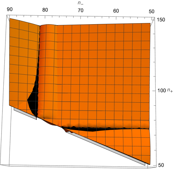
The hope of finding twist solutions with therefore rest on finding solutions with .1313 13 The case A numerical solution in Ferrero:2021etw is indeed in this class with . The constraints for the roots to have the correct form allows for three regimes which may be found below. Imposing on top that the scalars are positive definite leads to a far more constrained system, which is also more difficult to write down due to a larger number of possibilities and redundancies. However, by first studying the solutions for just the correct roots we find that for two of the three regimes only small islands of solutions can be found, see for example figure 2. Imposing on top of this the scalar positivity constraints leads to these islands vanishing for all charge configurations that we checked. We presume that in these two regimes there are no solutions but we have been able to rule this out completely. The third regime is far kinder to us and leads to infinite families of solutions, reminiscent of how simple it was to find the anti-twist solutions. The three regimes for solutions with the correct root structure are given below. It is the third regime where we can find infinite families of solutions and therefore we will focus on that case.
Regime 1 The first regime has a strictly positive subject to the inequalities
| (5.1) | ||||
Regime 2 The second regime allows for both a positive and negative subject to
| (5.2) | ||||
Regime 3 The third and final regime has a strictly negative satisfying
| (5.3) | ||||
5.1 Infinite families of solutions
This final regime requires an odd number of positive charges since . For the anti-twist solutions we had in the bountiful region. We are once again able to find infinite numbers of solutions for generic seed magnetic charges which are all negative. Amazingly we find that for any seed solution with all three magnetic charges negative any choice of gives a valid solution. Some of the explicit configurations that we have checked are
| (5.4) |
though there are plenty more with higher and higher orders. The important constraint is that all three seed charges are negative and it follows that we end up with three negative and one positive magnetic charge. Though we did not algebraically prove this the large number of data points we have tested indicates that this should true and we conclude that infinite families of solutions exist for three negative and one positive magnetic charges for . Note that this analysis agrees with the fact that in neither Einstein–Maxwell nor the truncation one can find a twist solution as shown in Ferrero:2021etw; Couzens:2021rlk. In these truncations the quartic polynomial is simple enough that one can prove this fully algebraically.
Given the flip symmetry we can obtain solutions where by taking three positive seed magnetic charges and one negative. We have checked this explicitly and the bounds agree with the transformed ones discussed above,
We finish this section by giving the closed form expression for the free-energy for twist solutions,
| (5.5) |
We emphasise that this is distinct to the expression for the anti-twist free-energy by three signs.
6 Conclusion
We have studied the possibility of realising both the twist and anti-twist for the multi-charge AdS solutions. We have constructed infinite classes of both solutions, parametrised by the choice of seed magnetic charges, providing insurmountable evidence for their existence, in agreement with Ferrero:2021etw. For twist solutions we find infinite families of solutions when three of the four magnetic charges are either all positive or all negative. Whilst for anti-twist solutions we find that all magnetic charges are either positive or all negative with the sign correlated to the magnitude of the orbifold weights. It would be interesting to prove that these are the only possibilities. A non-extensive numerical analysis seems to confirm this but we were unable to present an algebraic proof.
We have provided compact and explicit expressions for the free-energy of the solutions expressed in terms of the magnetic charges and orbifold weights. In Faedo:2021nub, they conjectured a form for the off-shell free-energy wrapped brane spindle solutions in various dimensions. Their conjecture for the off-shell free energy for M2-branes is1414 14 We have rewritten the charges into our notation and swapped the definitions of and in Faedo:2021nub for consistency with our notation.
| (6.1) |
where
| (6.2) |
and, like here the charges satisfy the constraint
| (6.3) |
As explained in Faedo:2021nub this should be extremised for and subject to the constraint between and . The parameter is a fugacity associated to the rotational symmetry of the spindle whilst the are fugacities for the U symmetry. It is a feature of the spindle (and disc) geometries that the R-symmetry mixes with the rotational symmetries of the compactification surface and therefore requires the inclusion of the fugacity which would not otherwise appear for a static geometry like the ones we are considering here.
Given our expressions we find that the free-energy of the multi-charge spindle solutions for twist and anti-twist solutions can be written as
| (6.4) |
It would be interesting to recover this result from extremising the above functional and to understand how this latter constraint arises.
Acknowledgments
It is a pleasure to thank Hyojoong Kim, Nakwoo Kim, Yein Lee, Myungbo Shim, Minwoo Suh, Koen Stemerdink and Damian van de Heisteeg for useful discussions. I would also like to thank Pietro Ferrero, Jerome Gauntlett and James Sparks for comments on an earlier version of the draft and Andrea Boido for pointing out a typo. CC is supported by the National Research Foundation of Korea (NRF) grant 2019R1A2C2004880.
Appendix A Killing spinors on the spindle
In this section we will study the Killing spinors of the four-dimensional solution. For the conventions of the supersymmetry transformations we take the general form of the Killing spinor equations of 4d gauged supergravity in Lauria:2020rhc with the prepotential
| (A.1) |
We work in the gauge where
| (A.2) |
and define the physical scalars via
| (A.3) |
with
| (A.4) |
The resultant gravitino Killing spinor equation is1515 15 The Killing spinor equations are given in terms of symplectic Majorana spinors, with of positive chirality and of negative chirality. It is convenient to rewrite the Killing spinor equations in terms of the Dirac spinor , which we will take from now on.
| (A.5) |
whilst the three gaugino Killing spinor equations are
| (A.6) |
Working in components, on AdS2 we find ()
| (A.7) |
with the covariant derivative on unit radius AdS2 and the curved indices with respect to the conformally rescaled metric which removes the overall conformal factor in (2.3). The parameter is either depending on whether or . This is related to the two different ways of enforcing positive scalars. The other two Killing spinor are
| (A.8) | ||||
| (A.9) |
We have allowed for an arbitrary gauge choice for the gauge fields parametrised by the , see Ferrero:2021etw for a detailed discussion of gauge choices.
Let us now solve these conditions. From the Killing spinor equation along AdS2 we see that we must impose that the spinor satisfies the projection condition
| (A.10) |
which implies
| (A.11) |
Let us take the gamma matrices
| (A.12) |
then , with the 2d gamma matrices for AdS2 and therefore the Killing spinor on AdS2 reduces to
| (A.13) |
We should decompose the 4d spinor in terms of AdS2 Killing spinors. There are two inequivalent Killing spinor equations that we can construct depending on the sign of . In terms of these spinors we can decompose the 4d spinors as1616 16 The index of the ’s confers no information about a projection.
| (A.14) |
with solving (A.13) for and solving (A.13) for . If we put the following metric on AdS2
| (A.15) |
then the Killing spinors on AdS2 are
| (A.16) |
We may now solve the Killing spinor equations by first solving the projection condition, and then solving for the remaining component.
Let us first consider . We expect to construct a spinor utilising the spinor on AdS2. We find the solution
| (A.17) |
For we find that the AdS2 spinor we must take is and the spinor is
| (A.18) |
Note that these spinors agree with the ones found in Ferrero:2021etw once the simple redefinitions mapping between the two solutions are imposed.
Let us now consider the differences between the two types of twist. Since we can restrict to considering only without loss of generality. First note that the product of the entries of the spinor is precisely the function that is
| (A.19) |
Recall that at a root, of we have
| (A.20) |
Therefore we see that at one of the poles of the spindle one entry of the spinor vanishes, but not both. Let us reinstate the two roots, and . Then at we have
| (A.21) |
whilst at we have
| (A.22) |
We therefore see that the twist and anti-twist solutions have Killing spinors with different properties.1717 17 Note that the disc preserves supersymmetry in an altogether different way since at the boundary of the disc, located at , the Killing spinor vanishes as .
Appendix B Full black hole solution
We present a full black hole solution with near-horizon given by the solution studied in the main text. Having presented the full black hole solution we take the near-horizon limit and with a change of coordinates show that it recovers the near-horizon solution studied in the main text. We will not check explicitly the supersymmetry of the full black hole solution, instead we will require that it is extremal and has the supersymmetric solution studied in the main text as near-horizon geometry. Of course this is necessary but not sufficient for the full black hole solution to preserve supersymmetry however we will content ourselves with this in this work.
The solution was originally found in Lu:2014sza and was conjectured to give rise to the near-horizon solutions we study in this work in Ferrero:2021ovq. Dualising the solution Lu:2014sza to have only magnetic charges we have1818 18 We have changed the definitions of some of the functions and parameters to remove some of the redundancy in the definitions and potential confusion with previous expressions.
| (B.1) | ||||
with
| (B.2) | ||||
The solution depends on 9 parameters: 4 , 4 and , whilst can be fixed by a coordinate transformation, this will become important later. We will set the coupling constant to 1 as in the main text. Imposing supersymmetry will reduce the number of parameters down to 4 in the near-horizon. The form of the solution is reminiscent of the near-horizon solution studied in the main text and it is therefore reasonable that this gives rise to the solution in (2.3)-(2.6).
B.1 Near-Horizon limit
To obtain an AdS2 near-horizon geometry we should find a double root of the function and then expand around this point. Since is a quartic this is somewhat non-trivial, however in keeping with the results in the main text we do not need to solve for the roots, to take the limit. Instead we will assume the existence of a double root and show that with this assumption we can uniquely fix the near-horizon geometry by “shooting” for the near-horizon geometry in (2.3)-(2.6).
Let us fix a double root of to be , therefore we have
| (B.3) |
We can now expand the black hole solution around the horizon. The metric becomes
| (B.4) |
After a coordinate redefinition it takes the form
| (B.5) |
where
| (B.6) |
In comparing with (2.3) we identify
| (B.7) |
Next consider the coefficient of , comparing with (2.3) we find
| (B.8) |
and by equating the term and the term in (2.3) we find
| (B.9) |
With these definitions the metric takes the same form as in (2.3). It remains to check the other fields and that the expressions for and are actually consistent with the change of coordinates in (B.9) and the expressions for and in the main text.
Next, the scalars are shown to be equivalent in the near-horizon limit provided
| (B.10) |
The parameters are fixed by studying the gauge fields, and we find
| (B.11) |
Note that a relation between and is to be expected if the full black hole was supersymmetric and therefore this is quite natural from this point of view. In fact one sees that these relations turn out to be equivalent to getting a double root1919 19 One can show that after applying the solution for . , and therefore one should think of this as the extremal condition for the black hole. We therefore have that the near-horizon limit of the black hole solution in (B.1) takes the correct general form of the solution studied in the main text. What remains to be checked is that the definitions of and are consistent with the form of and in the main text respectively. It turns out that checking gives the correct form for is straightforward. By substituting in the change of coordinates (B.9) and (B.10) one simply lands on the correct form for and therefore it is consistent, for and this is not as simple.
Firstly, we set and which implies that the first two terms in cancel. After a little rewriting we find that takes the form
| (B.12) |
with some coefficients. At first these coefficients look particularly unwieldy however we may express them in terms of and its derivatives. We find
| (B.13) |
From the assumption of a double root we see that immediately and amazingly after using the definition of in (B.11) vanishes also. Therefore only remains and is simply given by
| (B.14) |
after using (B.6). Setting
| (B.15) |
which we are inclined to assume is the final constraint from supersymmetry, implies
| (B.16) |
and therefore all the definitions are consistent and the near-horizon limit agrees on the nose with the solution discussed in the main text. We conclude that the supersymmetric limit of the asymptotically AdS4 black hole found in Lu:2014sza and given in (B.1), gives rise to the AdS2 geometries studied in this work in the near-horizon limit.
References
- (1) P. Ferrero, J. P. Gauntlett, J. M. Pérez Ipiña, D. Martelli and J. Sparks, D3-Branes Wrapped on a Spindle, Phys. Rev. Lett. 126 (2021) 111601, [2011.10579].
- (2) P. Ferrero, J. P. Gauntlett, J. M. P. Ipiña, D. Martelli and J. Sparks, Accelerating black holes and spinning spindles, Phys. Rev. D 104 (2021) 046007, [2012.08530].
- (3) S. M. Hosseini, K. Hristov and A. Zaffaroni, Rotating multi-charge spindles and their microstates, JHEP 07 (2021) 182, [2104.11249].
- (4) F. Faedo and D. Martelli, D4-branes wrapped on a spindle, 2111.13660.
- (5) C. Couzens, K. Stemerdink and D. van de Heisteeg, M2-branes on Discs and Multi-Charged Spindles, 2110.00571.
- (6) P. Ferrero, M. Inglese, D. Martelli and J. Sparks, Multi-charge accelerating black holes and spinning spindles, 2109.14625.
- (7) F. Faedo, S. Klemm and A. Viganò, Supersymmetric black holes with spiky horizons, JHEP 09 (2021) 102, [2105.02902].
- (8) P. Ferrero, J. P. Gauntlett and J. Sparks, Supersymmetric spindles, 2112.01543.
- (9) D. Cassani, J. P. Gauntlett, D. Martelli and J. Sparks, Thermodynamics of accelerating and supersymmetric AdS4 black holes, Phys. Rev. D 104 (2021) 086005, [2106.05571].
- (10) A. Boido, J. M. P. Ipiña and J. Sparks, Twisted D3-brane and M5-brane compactifications from multi-charge spindles, JHEP 07 (2021) 222, [2104.13287].
- (11) P. Ferrero, J. P. Gauntlett, D. Martelli and J. Sparks, M5-branes wrapped on a spindle, JHEP 11 (2021) 002, [2105.13344].
- (12) I. Bah, F. Bonetti, R. Minasian and E. Nardoni, Holographic Duals of Argyres-Douglas Theories, Phys. Rev. Lett. 127 (2021) 211601, [2105.11567].
- (13) I. Bah, F. Bonetti, R. Minasian and E. Nardoni, M5-brane sources, holography, and Argyres-Douglas theories, JHEP 11 (2021) 140, [2106.01322].
- (14) C. Couzens, N. T. Macpherson and A. Passias, AdS3 from D3-branes wrapped on Riemann surfaces, 2107.13562.
- (15) M. Suh, D3-branes and M5-branes wrapped on a topological disc, 2108.01105.
- (16) M. Suh, D4-D8-branes wrapped on a manifold with non-constant curvature, 2108.08326.
- (17) M. Suh, M2-branes wrapped on a topological disc, 2109.13278.
- (18) C. Couzens and K. Stemerdink, Spinning discs, to appear (2022) .
- (19) J. P. Gauntlett, N. Kim and D. Waldram, Supersymmetric AdS(3), AdS(2) and Bubble Solutions, JHEP 04 (2007) 005, [hep-th/0612253].
- (20) M. Cvetic, M. J. Duff, P. Hoxha, J. T. Liu, H. Lu, J. X. Lu et al., Embedding AdS black holes in ten-dimensions and eleven-dimensions, Nucl. Phys. B 558 (1999) 96–126, [hep-th/9903214].
- (21) J. P. Gauntlett and N. Kim, Geometries with Killing Spinors and Supersymmetric AdS Solutions, Commun. Math. Phys. 284 (2008) 897–918, [0710.2590].
- (22) N. Kim and J.-D. Park, Comments on AdS(2) solutions of D=11 supergravity, JHEP 09 (2006) 041, [hep-th/0607093].
- (23) O. A. P. Mac Conamhna and E. O Colgain, Supersymmetric wrapped membranes, AdS(2) spaces, and bubbling geometries, JHEP 03 (2007) 115, [hep-th/0612196].
- (24) E. Lauria and A. Van Proeyen, Supergravity in Dimensions, vol. 966. 3, 2020, 10.1007/978-3-030-33757-5.
- (25) H. Lü and J. F. Vázquez-Poritz, C-metrics in Gauged STU Supergravity and Beyond, JHEP 12 (2014) 057, [1408.6531].