The rare second-class decay mode of the $\tau$ into $\eta\pi\nu$ could be observed for the first time at Belle II. It is important to try to derive a reliable evaluation of the branching fraction and of the energy distribution of this mode within the standard-model. Many predictions exist already in the literature which can differ by one to two orders of magnitude. Here, an approach based on a systematic use of the property of analyticity of form factors and scattering amplitudes in QCD is discussed. In particular, we will show that the scalar form factor in the $\tau$ decay can be related to photon-photon scattering and radiative $\phi$ decay amplitudes for which precise experimental measurements have been performed by the Belle and KLOE collaborations.

The decay $\tau\to\eta\pi\nu$ is induced by second-class type currents [1]. In the Standard Model (SM) the amplitude must thus be proportional to the small isospin breaking parameters: $(m_{d}-m_{u})/m_{s}$, $e^{2}$ and it has a sensitivity to new scalar or tensor interactions (e.g. [2, 3, 4]). As Tony Pich has reminded us in the introductory talk, this mode was once claimed to have been observed [5] with an unexpectedly large branching fraction $BF=(5.1\pm 1.5)\%$ but this was not confirmed. The best upper bounds now available are $BF<7.3\times 10^{-5}$ (Belle [6]) and $BF<9.9\times 10^{-5}$ (Babar [7]). At the new Belle II facility, it has been estimated [8] that the $\tau\to\eta\pi\nu$ decay could be observed with a significance of $2.6\sigma$ for a branching fraction of $4.4\times 10^{-5}$. A second-class scalar current would lead to a simple modification of the scalar form factor (defined below (2)) by a term linear in energy

$$f_{0}^{\eta\pi}(s)=\left.f_{0}^{\eta\pi}(s)\right|_{SM}\left(1-\epsilon_{S}\frac{s}{m_{\tau}(m_{d}-m_{u})}\right)$$

(1)

proportional to the strength $\epsilon_{S}$ (with the notation of [9]) of the new interaction. A correct estimate of the scalar form factor in the SM is necessary in order to derive reliable constraints on $\epsilon_{S}$ from experimental results.

A number of evaluations of the $\eta\pi$ vector and scalar form factors have already been performed (e.g. [10, 11, 12, 3, 13, 14, 15, 16] for a representative list). The predictions for the branching fraction associated with the vector form factor lie in a range $BF_{V}\simeq[0.1-0.8]\cdot 10^{-5}$ while those associated with the scalar form factor seem more uncertain: $BF_{S}\simeq[0.3-5.3]\cdot 10^{-5}$.

We present here an evaluation of $f_{0}^{\eta\pi}$ which exploits the properties of analyticity and unitarity of form factors in QCD (e.g. [17]). In this framework, generating the energy dependence of the form factors can be viewed as a final-state interaction (FSI) problem. This allows us to derive relations between the scalar form factor and the photon-photon production amplitude $\gamma\gamma\to\eta\pi$ and also with the $\phi$ radiative decay amplitude $\phi\to\gamma\eta\pi$, for which FSI theory can also be applied and which are experimentally known.

The $\tau$ decay amplitude into two pseudoscalar mesons involves the matrix element of the charged vector current ${\langle P_{1}(p_{1})P_{2}(p_{2})|j_{\mu}^{uq}(0)|0\rangle}$ (with $j_{\mu}^{uq}=\bar{u}{}_{\mu}{q}$, $q=d,s$), which can be expressed in terms of two independent form factors

$${\langle P_{1}(p_{1})P_{2}(p_{2})|\bar{u}{}^{\mu}{q}|0\rangle}=C_{12}\Big\{f_{+}^{P_{1}P_{2}}(s)\Big[p_{1}-p_{2}-\frac{\Delta_{12}}{s}(p_{1}+p_{2})\Big]^{\mu}+f_{0}^{P_{1}P_{2}}(s)\,\frac{\Delta_{12}}{s}[p_{1}+p_{2}]^{\mu}\Big\}$$

(2)

where $s=(p_{1}+p_{2})^{2}$, $\Delta_{12}=m_{1}^{2}-m_{2}^{2}$ and $C_{12}$ is a numerical factor (below, we will need $C_{\eta\pi^{+}}=-\sqrt{2}$, $C_{\bar{K}^{0}{K^{+}}}=-1$). Using the Ward identity for the vector current, the scalar form factors $f_{0}^{P_{1}P_{2}}$ can also be expressed in terms of the matrix elements,

$$C_{12}\Delta_{12}f_{0}^{P_{1}P_{2}}(s)=-{\langle P_{1}(p_{1})P_{2}(p_{2})|(m_{d}-m_{u})\bar{u}d-eA_{\mu}{j}^{\mu,ud}|0\rangle}\ .$$

(3)

For the $\pi\pi$ or $\pi{K}$ vector form factors, simple approximate evaluations are known to hold e.g.

$$f_{+}^{\pi K}(s)\simeq f_{+}^{\pi K}(0){}_{1}(s),\quad{}_{1}(s)=\exp\Big(\frac{s}{\pi}\int_{(m_{\pi}+m_{K})^{2}}^{\infty}ds^{\prime}\,\frac{\delta^{1/2}_{1}(s^{\prime})}{s^{\prime}(s^{\prime}-s)}\Big)$$

(4)

where ₁ is the Omnès function [18] and $\delta^{1/2}_{1}$ is the $J=0$ $I=1/2$ $\pi{K}$ scattering phase shift. This is justified because $\pi{K}$ scattering is effectively elastic in a energy region $s<\Lambda^{2}$, with $\Lambda\simeq 1$ GeV, which includes the leading low energy resonance $K^{*}(892)$. Multiplying $f_{+}^{\pi K}$ by the inverse of the Omnès function removes the cut below $\Lambda$, such that in the region $s<\Lambda^{2}$ one can write a low energy expansion: ${}^{-1}(s)f_{+}^{\pi K}(s)=f_{+}^{\pi K}(0)(1+O(s/\Lambda^{2}))$. The situation is different for the $\pi\eta$ vector form factor because contributions to unitarity arise form the states ${|\gamma\pi^{+}\rangle}$, ${|\pi^{0}\pi^{+}\rangle}$ which are lighter than the elastic threshold ${|\eta\pi^{+}\rangle}$. The contribution from the ${|\pi^{0}\pi^{+}\rangle}$ should be the dominant one below 1 GeV as it is enhanced by the $\rho(770)$ resonance. The corresponding discontinuity reads,

$${\rm disc\,}[f_{+}^{\pi\eta}(s)]_{\pi\pi}=2i\theta(s-4{m^{2}_{\pi}})\frac{4{m^{2}_{\pi}}-s}{\sqrt{\lambda_{\eta\pi}(s)}}F_{V}^{\pi}(s)\times(t_{J=1}^{\pi^{0}\pi^{+}\to\eta\pi^{+}}(s))^{*}$$

(5)

where $\lambda_{12}(s)=(s-(m_{1}+m_{2})^{2})(s-(m_{1}-m_{2})^{2})$. It involves the pion form factor (which is well measured) and the $J=1$ projection of the $\pi\pi\to\eta\pi$ amplitude. This amplitude was evaluated in [15] using Khuri-Treiman equations with experimental inputs on $\eta\to 3\pi$ decays.

Let us now consider the scalar form factor $f_{0}^{\pi\eta}$. In that case, the ${|\pi^{0}\pi^{+}\rangle}$ contribution to unitarity can be neglected because it is quadratic in isospin breaking. The important low energy scalar resonance is the $a_{0}(980)$ which is known to couple strongly to the two channels ${|\eta\pi^{+}\rangle}$ and ${|\bar{K}^{0}{K^{+}}\rangle}$. The unitarity relation for the scalar form factor, including these two channels, reads (see ref. [15] for details on the derivation)

$$\begin{array}[]{ll}{\rm Im\,}[f_{0}^{\eta\pi^{+}}(s)]&=\sigma_{\eta\pi^{+}}(s)\,f_{0}^{\eta\pi^{+}}(s)\times(t^{\eta\pi^{+}\to\eta\pi^{+}}_{J=0}(s))^{*}\\[8.5359pt] &+\sigma_{\bar{K}^{0}{K^{+}}}(s)\,\dfrac{\Delta_{\bar{K}^{0}{K^{+}}}}{\sqrt{2}{\Delta_{\eta\pi}}}f_{0}^{\bar{K}^{0}{K^{+}}}(s)\times(t^{\eta\pi^{+}\to\bar{K}^{0}{K^{+}}}_{J=0}(s))^{*}\end{array}$$

(6)

where $\sigma_{12}(s)=\theta(s-(m_{1}+m_{2})^{2})\sqrt{\lambda_{12}(s)}/{s}$ and a similar relation can be written for ${\rm Im\,}[f_{0}^{\bar{K}^{0}{K^{+}}}]$. This suggests a minimal representation of the scalar form factors analogous to eq. (4) involving an Omnès matrix instead of a function,

$$\begin{pmatrix}f_{0}^{\eta\pi^{+}}(s)\\[5.69046pt] \epsilon_{KK}f_{0}^{\bar{K}^{0}{K^{+}}}(s)\end{pmatrix}\simeq\begin{pmatrix}{}_{11}(s)&{}_{12}(s)\\[2.84544pt] {}_{21}(s)&{}_{22}(s)\end{pmatrix}\begin{pmatrix}f_{0}^{\eta\pi^{+}}(0)\\[2.84544pt] \epsilon_{KK}f_{0}^{\bar{K}^{0}{K^{+}}}(0)\end{pmatrix}$$

(7)

with¹¹ 1 The minus sign arises because the $\Omega$ matrix is defined with respect to isospin eigenstates and one has ${|\eta\pi^{+}\rangle}=-{|1,1\rangle}$. $\epsilon_{KK}=-\Delta_{\bar{K}^{0}{K^{+}}}/\sqrt{2}\Delta_{\eta\pi}$. The coupled-channel Omnès-Muskhelishvili problem cannot be solved in closed form in terms of phase-shifts and inelasticities as in the one-channel case, but the equations can be solved numerically in terms of the $T$-matrix elements [19]. Furthermore, no direct experimental determinations of the phase-shifts and inelasticities has been performed for $\eta\pi$ scattering.

Cross-sections for $\gamma\gamma\to\eta\pi^{0}$ have first been measured by the Crystal Ball collaboration at SLAC [20] and at DESY [21]. Recently, high statistics measurements have been performed by the Belle collaboration [22]. The $\gamma\gamma\to\eta\pi^{0}$ process is described by helicity amplitudes $L_{\lambda\lambda^{\prime}}$ which are functions of the Mandelstam variables $s$ (the energy squared of the $\eta\pi^{0}$ pair) and $t$, $u$. In the energy region $\sqrt{s}\mathrel{\raise 2.58334pt\hbox{$<$}\kern-7.7778pt\lower 2.79857pt\hbox{$\sim$}}1.4$ GeV the contributions of the partial waves with $J>2$ to the cross-sections are negligibly small, while in the region $\sqrt{s}\mathrel{\raise 2.58334pt\hbox{$<$}\kern-7.7778pt\lower 2.79857pt\hbox{$\sim$}}1.1$ GeV, the $S$-wave $l_{0++}(s)$ dominates. Theoretical descriptions of this amplitude based on general FSI methods have been discussed recently [23, 24]. A closely related, but somewhat less general approach, was used earlier in ref. [25]. $l_{0++}(s)$ is an analytic function of $s$ except for two cuts.

The right-hand cut $s>(m_{\eta}+m_{\pi})^{2}$, as in the case of the form factor, is associated with unitarity. We will consider an energy region in which two-channel unitarity is a reasonable approximation such that one can write

$$\begin{array}[]{l}{\rm Im\,}[l_{0++}(s)]=\sigma_{\eta\pi^{0}}(s)\,l_{0++}(s)\,T_{11}^{*}(s)+\sigma_{K\bar{K}}(s)\,k^{1}_{0++}(s)\,T_{12}^{*}(s)\\ {\rm Im\,}[k^{1}_{0++}(s)]=\sigma_{\eta\pi^{0}}(s)\,l_{0++}(s)\,T_{12}^{*}(s)+\sigma_{K\bar{K}}(s)\,k^{1}_{0++}(s)\,T_{22}^{*}(s)\end{array}$$

(8)

where $k^{1}_{0++}(s)$ is the $J=0$ $\gamma\gamma\to(K\bar{K})^{I=1}$ amplitude and the $T$-matrix elements associated with the states ${|\eta\pi^{0}\rangle}$, ${|K\bar{K}\rangle}$ are denoted simply as $T_{ij}$. In addition to the right-hand cut, the amplitudes $l_{0++}(s)$, $k^{1}_{0++}(s)$ have a left-hand cut on the negative real axis $-\infty<s\leq 0$. There are no other singularities. The amplitudes must also satisfy Low’s soft photon theorem [26] which states that

$$\lim_{s\to 0}l_{0++}(s)=0,\quad\lim_{s\to 0}\bar{k}^{1}_{0++}(s)=0$$

(9)

where $\bar{k}^{1}_{0++}\equiv k^{1}_{0++}(s)-k^{1,Born}_{0++}(s)$ and $k^{1,Born}_{0++}$ is the $I=1$ projection of the amplitude part induced by the Kaon pole in the $t$ and $u$ channels, which coincides with the QED Born amplitude

$$k^{1,Born}_{0++}(s)=-\frac{2\sqrt{2}{m}^{2}_{K^{+}}}{s\sigma_{K^{+}}(s)}\log\frac{1+\sigma_{K^{+}}(s)}{1-\sigma_{K^{+}}(s)}\ .$$

(10)

and $\sigma_{K^{+}}(s)=\sqrt{1-4{m^{2}_{K^{+}}}/s}$. Knowing the location of the singularities allows one to write Cauchy dispersive integral representations ²² 2 It is also necessary to know the asymptotic behaviour. It can be argued [24] that $|l_{0++}(s)|$, $|k^{1}_{0++}(s)|$ are bounded by $\sqrt{s}$ when $s\to\infty$. for $l_{0++}$ and $k^{1}_{0++}$. Combining these with the unitarity relations (8) leads to a set of Muskhelishvili-type singular equations for the amplitudes. The solutions, taking into account the soft photon constraints, can be expressed in the following form in terms of the Omnès matrix [24]

$$\begin{pmatrix}l_{0++}(s)\\[4.26773pt] k^{1}_{0++}(s)\\ \end{pmatrix}=\begin{pmatrix}0\\[4.26773pt] k^{1,Born}_{0++}(s)\\ \end{pmatrix}+s\begin{pmatrix}{{}_{11}(s)}&{{}_{12}(s)}\\[4.26773pt] {{}_{21}(s)}&{{}_{22}(s)}\\ \end{pmatrix}\begin{pmatrix}{b_{l}}+L_{1}^{V}(s)+R_{1}^{Born}(s)\\[4.26773pt] {b_{k}}+L_{2}^{V}(s)+R_{2}^{Born}(s)\\ \end{pmatrix}\ .$$

(11)

In these equations the functions $R_{i}^{Born}$ are integrals involving the Born amplitude,

$$R_{i}^{Born}(s)=-\frac{s-s_{A}}{\pi}\int_{4{m^{2}_{K^{+}}}}^{\infty}\frac{ds^{\prime}}{s^{\prime}(s^{\prime}-s_{A})(s^{\prime}-s)}{\rm Im\,}[({}^{-1})_{i2}(s^{\prime})]k^{1,Born}_{0++}(s^{\prime})$$

(12)

where $s_{A}$ can conveniently be taken to be equal to the Adler zero of the amplitude $l_{0++}$ ($s_{A}\simeq m^{2}_{\eta}$) and the functions $L_{i}^{V}(s)$ are integrals over the left-hand cut involving ${\rm Im\,}[l_{0++}(s^{\prime})]$, ${\rm Im\,}[\bar{k}^{1}_{0++}(s^{\prime})]$. These imaginary parts are approximated by the contributions induced by the light vector meson poles in the $t$ (or $u$) channels, i.e.

$${\rm Im\,}[l_{0++}(s^{\prime})]\simeq\sum_{V=\rho,\omega,\phi}{\rm Im\,}[l^{V}_{0++}(s^{\prime})],\quad{\rm Im\,}[\bar{k}^{1}_{0++}(s^{\prime})]\simeq{\rm Im\,}[\bar{k}^{1,K^{*}}_{0++}(s^{\prime})],\quad(s^{\prime}\leq 0)\ .$$

(13)

As before, the contributions from the higher energy regions of the cuts, where the approximations made are no longer accurate, are absorbed into a set of subtraction parameters. Eq. (11) involves two such parameters $b_{l}$, $b_{k}$.

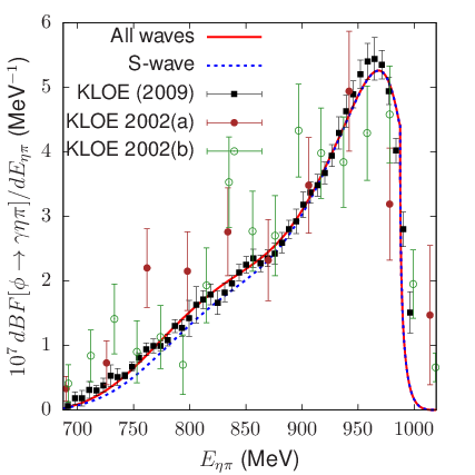
The representation (11) for the $S$-wave $\gamma\gamma$ amplitudes, supplemented with a simple Breit-Wigner model for the $D$-waves, was compared to the experimental data on photon-photon scattering to $\eta\pi$ cross-sections in [23, 24]. In ref. [24] experimental data on $\gamma\gamma\to K_{S}K_{S},{K^{+}}{K^{-}}$ was considered as well, which allows to constrain not only the constants $b_{l}$, $b_{k}$ but also the $\Omega$ matrix. For that purpose, a previously proposed six parameters model for the underlying $T$-matrix [27] was used, from which $\Omega$ is computed by solving numerically the related Muskhelishvili-Omnès equations. Fig. (1) shows an illustrative comparison of cross sections computed from this fitted theoretical model with the experimental ones.

Let us now consider the case where one photon has a non-vanishing virtuality ${q^{2}}$, and label the $S$-wave amplitudes as $l_{0++}(s,{q^{2}})$, $k^{1}_{0++}(s,{q^{2}})$. These amplitudes are analytic functions of the energy $s$ with two cuts (there are no anomalous thresholds), such that one can write a dispersive representation in terms of the Omnès matrix, exactly as before,

$$\begin{pmatrix}l_{0++}(s,{q^{2}})\\ k_{0++}(s,{q^{2}})\end{pmatrix}\!=\!\begin{pmatrix}0\\ \tilde{k}^{1,Born}(s,{q^{2}})\end{pmatrix}\!\!+(s-{q^{2}})\begin{pmatrix}\!\!{{}_{11}}(s)&{{}_{12}}(s)\\ {{}_{21}}(s)&{{}_{22}}(s)\end{pmatrix}\!\!\begin{pmatrix}{a_{1}}({q^{2}})+I_{1}^{LC}(s,{q^{2}})+I_{1}^{RC}(s,{q^{2}})\\ {a_{2}}({q^{2}})+I_{2}^{LC}(s,{q^{2}})+I_{2}^{RC}(s,{q^{2}})\end{pmatrix}\$$

(14)

satisfying the soft photon theorem which now corresponds to $s={q^{2}}$. We will be interested in the case of timelike virtualities and ${q^{2}}>(m_{\eta}+m_{\pi})^{2}$ which corresponds experimentally to the $e^{+}e^{-}\to{}^{*}\to\gamma\eta\pi$ processes (and also, up to an isospin rotation, to the vector current part of the radiative $\tau$ decays $\tau^{+}\to\gamma\eta\pi^{+}\nu,\gamma\bar{K}^{0}K^{+}\nu$). Some care must be taken in order to properly utilize eq. (14) because the pole singularity of the Born amplitude at $s={q^{2}}$ occurs within the range of integration in the integrals $I^{RC}_{i}$. It is convenient to separate this singular part (labelled $\tilde{k}^{1,Born}$ in (14) )and perform the related integrations analytically. Furthermore, the left-hand cut now has complex components as well as a real component which partly overlaps with the unitarity cut (which leads to a violation of the Fermi-Watson phase theorem). Details on how to properly compute the left-cut integrals $I_{i}^{LC}$ can be found in [28]). In practice, eqs. (14) where implemented with ${q^{2}}\simeq m^{2}_{\phi}$ enabling to determine the $\phi(1020)\to\gamma\eta\pi$ decay amplitude. As in the ${q^{2}}=0$ case, the discontinuities across the left-hand cut components are modelled based on the contributions from the light vector mesons $\rho$, $\omega$, $\phi$ and $K^{*}$. Fig. (1) shows that a rather good description of the accurate experimental data [29, 30] can be obtained with a two parameter fit, using the $\Omega$ matrix as determined previously from the $\gamma\gamma$ scattering fit.

In the minimal modelling, once the $\Omega$ matrix is known the scalar form factors are given in terms of their values at $s=0$. Since $f_{0}^{\bar{K}^{0}{K^{+}}}(0)$ appears multiplied by an isospin breaking factor, we can simply set $f_{0}^{\bar{K}^{0}{K^{+}}}(0)=1$, because the chiral corrections are $O(m_{d}-m_{u},e^{2})$. The chiral expansion of $f_{0}^{\eta\pi^{+}}(0)$ takes the following form [12]

$$f_{0}^{\eta\pi^{+}}(0)=\epsilon\times(1+O(p^{2}))+\frac{O(e^{2}p^{2})}{m^{2}_{\eta}-{m^{2}_{\pi}}},\quad\epsilon=\frac{\sqrt{3}(m_{d}-m_{u})}{4(m_{s}-\hat{m})}$$

(15)

with $\hat{m}=(m_{d}+m_{u})/2$. The value of $\epsilon$ from the FLAG revue [31] is $\epsilon=1.137(45)\cdot 10^{-2}$. The $O(p^{2})$ correction involves the chiral couplings $L_{7}$, $L_{8}$ which can be computed using the chiral expansions of the pseudo-scalar meson masses at NLO and the value the quark mass ratio $m_{s}/\hat{m}$ [32], which is known from lattice QCD simulations: $m_{s}/\hat{m}=27.42(12)$ (see [31]). The couplings which appear in the $O(e^{2}p^{2})$ part in (15) are not precisely known, they can be estimated approximately using resonance saturation modelling [33, 34]. Finally, from this NLO chiral expansion, one obtains

$$\left.f_{0}^{\eta\pi^{+}}(0)\right|_{\chi{PT}}=(1.40\pm 0.14)\cdot 10^{-2}\ ,$$

(16)

assuming a 50% error on the chiral corrections. An alternative estimate can be performed based on a relation, which is exact at NLO, with the $K^{+}_{l3}$ and $K^{0}_{l3}$ form factors ratio $\Delta_{SU(2)}$ $\equiv{f_{0}^{{K^{+}}\pi^{0}}(0)}/{f_{0}^{{K^{0}}\pi^{-}}(0)}-1$ [12]. The experimental value $\Delta_{SU(2)}$ $=(2.73\pm 0.41)\cdot 10^{-2}$ [35] gives $f_{0}^{\eta\pi^{+}}(0)|_{\chi{PT}+K_{l3}}$ $=(1.51\pm 0.24)\cdot 10^{-2}$ which is compatible with eq. (16). Using the values at $s=0$ from $\chi$pt the result for $f_{0}^{\eta\pi}(s)$ from the minimal Omnès representation is illustrated in Fig (2) (solid black line on the left plot). Obviously, this minimal model cannot be very precise. In fact, computing the derivatives of the form factors at $s=0$ one finds substantial deviations from the $O(p^{4})$ $\chi$pt values: $\dot{f}_{0}^{\eta\pi}(0)|_{min}/\dot{f}_{0}^{\eta\pi}(0)|_{\chi{pt}}\sim 0.5$, $\dot{f}_{0}^{K\bar{K}}(0)|_{min}/\dot{f}_{0}^{K\bar{K}}(0)|_{\chi{pt}}\sim 1.6$. The values of the derivatives can be corrected by replacing $f_{0}^{12}(0)$ in eq. (7) by a linear polynomial $f_{0}^{12}(0)(1+\lambda_{12}s)$. Physically, it is plausible that two-channel unitarity is insufficient in the region of the $a_{0}(1450)$ resonance. Assuming an effective third channel, this suggests the following simple improvement over the minimal model

$$f_{0}^{\eta\pi}(s)=\left.f_{0}^{\eta\pi}(s)\right|_{min}+{}_{13}(s)\lambda_{13},\quad{}_{13}(s)\simeq\frac{s}{m^{2}_{a_{0}^{\prime}}-s-im_{a_{0}^{\prime}}\Gamma_{a_{0}^{\prime}}}$$

(17)

in which the parameter $\lambda_{13}$ is adjusted such that the $\chi$pt derivative at $s=0$ is reproduced. The effects of these various ways to modify the derivatives at $s=0$ are illustrated in Fig. (2).

The energy dependence of the $\tau\to\eta\pi\nu$ branching fraction associated to the scalar form factor is shown in Fig. (2) (right). Also shown for comparison is the branching fraction associated with the vector form factor. The dotted red line is the result from ref. [15] in which the amplitude $t_{J=1}^{\pi^{0}\pi^{+}\to\eta\pi^{+}}$ is determined using $\eta\to 3\pi$ inputs from ref. [36]. The solid red line is an update which uses the more recent results from [37]. One sees a substantial difference between these two evaluations which gives a measure of the error. Finally, integrating over the $\pi\eta$ energy we find the following results for the branching fractions

$$BF_{S}=(1.8\pm 0.7)\cdot 10^{-6},\quad BF_{V}=(2.6\pm 1.30)\cdot 10^{-6}\ .$$

(18)

We have proposed a determination of the scalar form factor component of the $\tau\to\eta\pi\nu$ amplitude based on a two-channel Omnès matrix constrained by photon-photon scattering data and shown to be compatible with $\phi$ radiative decay data. The result for the branching fraction $BF_{S}$ (eq. (18)) should be more precise than the one given previously in [15] ³³ 3 In that reference and idea proposed in ref. [38] was followed, which consists in making estimates of the behavior of the phase of the form factor in the inelastic region using the QCD asymptotic constraint.. We have also presented an update on the branching fraction generated by the vector form factor. If our results are correct, then the forthcoming search for this rare $\tau$ decay mode at Belle II might not be able to clearly see it. However, these new measurements should be able to rule out some of the theoretical models.

This work is supported by the European Union’s Horizon2020 research and innovation programme (HADRON-2020) under the Grant Agreement n^∘ 824093.

References

- [1] S. Weinberg, Charge symmetry of weak interactions, Phys.Rev. 112, 1375 (1958), 10.1103/PhysRev.112.1375.
- [2] A. Bramon, S. Narison and A. Pich, The Process in and beyond QCD, Phys.Lett. B196, 543 (1987), 10.1016/0370-2693(87)90817-3.
- [3] S. Nussinov and A. Soffer, Estimate of the branching fraction , the , and non-standard weak interactions, Phys.Rev. D78, 033006 (2008), 10.1103/PhysRevD.78.033006, 0806.3922.
- [4] E. A. Garcés, M. Hernández Villanueva, G. López Castro and P. Roig, Effective-field theory analysis of the decays, JHEP 12, 027 (2017), 10.1007/JHEP12(2017)027, 1708.07802.
- [5] M. Derrick et al., Evidence for the Decay -neutrino, Phys. Lett. B 189, 260 (1987), 10.1016/0370-2693(87)91308-6.
- [6] K. Hayasaka, Second class current in analysis and measurement of from Belle: electroweak physics from Belle, PoS EPS-HEP2009, 374 (2009), 10.22323/1.084.0374.
- [7] P. del Amo Sanchez et al., Studies of and at BaBar and a search for a second-class current, Phys.Rev. D83, 032002 (2011), 10.1103/PhysRevD.83.032002, 1011.3917.
- [8] K. Ogawa, M. H. Villanueva and K. Hayasaka, Search for second-class currents with the decay into , PoS Beauty2019, 061 (2020), 10.22323/1.377.0061.
- [9] T. Bhattacharya, V. Cirigliano, S. D. Cohen, A. Filipuzzi, M. Gonzalez-Alonso, M. L. Graesser, R. Gupta and H.-W. Lin, Probing Novel Scalar and Tensor Interactions from (Ultra)Cold Neutrons to the LHC, Phys. Rev. D 85, 054512 (2012), 10.1103/PhysRevD.85.054512, 1110.6448.
- [10] S. Tisserant and T. Truong, Decay induced by Light Quark Mass Difference, Phys.Lett. B115, 264 (1982), 10.1016/0370-2693(82)90659-1.
- [11] A. Pich, ’Anomalous’ Production in Tau Decay, Phys.Lett. B196, 561 (1987), 10.1016/0370-2693(87)90821-5.
- [12] H. Neufeld and H. Rupertsberger, Isospin breaking in chiral perturbation theory and the decays and , Z.Phys. C68, 91 (1995), 10.1007/BF01579808.
- [13] N. Paver and Riazuddin, On meson dominance in the ‘second class’ decay, Phys.Rev. D82, 057301 (2010), 10.1103/PhysRevD.82.057301, 1005.4001.
- [14] M. Volkov and D. Kostunin, The decays and in the NJL model, Phys.Rev. D86, 013005 (2012), 10.1103/PhysRevD.86.013005, 1205.3329.
- [15] S. Descotes-Genon and B. Moussallam, Analyticity of isospin-violating form factors and the second-class decay, Eur. Phys. J. C74, 2946 (2014), 10.1140/epjc/s10052-014-2946-8, 1404.0251.
- [16] R. Escribano, S. Gonzalez-Solis and P. Roig, Predictions on the second-class current decays , Phys. Rev. D 94(3), 034008 (2016), 10.1103/PhysRevD.94.034008, 1601.03989.
- [17] G. Barton, Introduction to dispersion techniques in field theory, Lecture notes and supplements in physics. W.A. Benjamin, New York (1965).
- [18] R. Omnès, On the Solution of certain singular integral equations of quantum field theory, Nuovo Cim. 8, 316 (1958), 10.1007/BF02747746.
- [19] J. F. Donoghue, J. Gasser and H. Leutwyler, The Decay of a Light Higgs Boson, Nucl.Phys. B343, 341 (1990), 10.1016/0550-3213(90)90474-R.
- [20] C. Edwards et al., Production of and in Photon - Photon Collisions, Phys. Lett. B 110, 82 (1982), 10.1016/0370-2693(82)90957-1.
- [21] D. Antreasyan et al., Formation of and in Photon-photon Collisions, Phys. Rev. D33, 1847 (1986), 10.1103/PhysRevD.33.1847.
- [22] S. Uehara et al., High-statistics study of eta pi0 production in two-photon collisions, Phys.Rev. D80, 032001 (2009), 10.1103/PhysRevD.80.032001, 0906.1464.
- [23] I. Danilkin, O. Deineka and M. Vanderhaeghen, Theoretical analysis of the process, Phys. Rev. D96(11), 114018 (2017), 10.1103/PhysRevD.96.114018, 1709.08595.
- [24] J. Lu and B. Moussallam, The interaction and resonances in photon–photon scattering, Eur. Phys. J. C 80(5), 436 (2020), 10.1140/epjc/s10052-020-7969-8, 2002.04441.
- [25] J. A. Oller and E. Oset, Theoretical study of the gamma gamma meson - meson reaction, Nucl. Phys. A629, 739 (1998), 10.1016/S0375-9474(97)00649-0, hep-ph/9706487.
- [26] F. Low, Bremsstrahlung of very low-energy quanta in elementary particle collisions, Phys.Rev. 110, 974 (1958), 10.1103/PhysRev.110.974.
- [27] M. Albaladejo and B. Moussallam, Form factors of the isovector scalar current and the scattering phase shifts, Eur. Phys. J. C 75(10), 488 (2015), 10.1140/epjc/s10052-015-3715-z, 1507.04526.
- [28] B. Moussallam, Revisiting near the using analyticity and the left-cut structure, Eur. Phys. J. C 81(11), 993 (2021), 10.1140/epjc/s10052-021-09772-8, 2107.14147.
- [29] A. Aloisio et al., Study of the decay with the KLOE detector, Phys.Lett. B536, 209 (2002), 10.1016/S0370-2693(02)01821-X, hep-ex/0204012.
- [30] F. Ambrosino et al., Study of the meson via the radiative decay with the KLOE detector, Phys.Lett. B681, 5 (2009), 10.1016/j.physletb.2009.09.022, 0904.2539.
- [31] Y. Aoki et al., FLAG Review 2021 (2021), 2111.09849.
- [32] J. Gasser and H. Leutwyler, Chiral Perturbation Theory: Expansions in the Mass of the Strange Quark, Nucl.Phys. B250, 465 (1985), 10.1016/0550-3213(85)90492-4.
- [33] R. Baur and R. Urech, Resonance contributions to the electromagnetic low-energy constants of chiral perturbation theory, Nucl. Phys. B 499, 319 (1997), 10.1016/S0550-3213(97)00348-9, hep-ph/9612328.
- [34] B. Ananthanarayan and B. Moussallam, Four-point correlator constraints on electromagnetic chiral parameters and resonance effective Lagrangians, JHEP 06, 047 (2004), 10.1088/1126-6708/2004/06/047, hep-ph/0405206.
- [35] M. Antonelli, V. Cirigliano, G. Isidori, F. Mescia, M. Moulson et al., An Evaluation of and precise tests of the Standard Model from world data on leptonic and semileptonic kaon decays, Eur.Phys.J. C69, 399 (2010), 10.1140/epjc/s10052-010-1406-3, 1005.2323.
- [36] F. Ambrosino et al., Determination of Dalitz plot slopes and asymmetries with the KLOE detector, JHEP 0805, 006 (2008), 10.1088/1126-6708/2008/05/006, 0801.2642.
- [37] A. Anastasi et al., Precision measurement of the Dalitz plot distribution with the KLOE detector, JHEP 05, 019 (2016), 10.1007/JHEP05(2016)019, 1601.06985.
- [38] F. Ynduráin, The Quadratic scalar radius of the pion and the mixed pi-k radius, Phys.Lett. B578, 99 (2004), 10.1016/j.physletb.2003.10.037, 10.1016/j.physletb.2004.03.001, hep-ph/0309039.