Analytical model of low mass strange stars in 2+1 spacetime
Abstract
The low mass compact stars are quite fascinating objects to study for their enigmatic behaviour. In this paper, we have modeled this kind of low mass strange stars based on the Heintzmann ansatz [1] in dimension. Attractive anisotropic force plays a significant role to restrict the upper mass limit (which is comparatively low) of the strange star. We have applied our model to some low mass strange stars. Our model could be useful to predict the important parameters of the low mass strange stars.
Introduction
The peculiar behaviour of some compact stars opens the door of the possibility of the low mass neutron stars and the low mass strange stars. One can explain the high braking index of the PSR J1640-4631 [2] and the smaller polar cap area of the PSR B0943+10 [3] by considering that we can say these are low mass strange stars. Though theoretically, the low mass compact stars could be a product of a core-collapse supernova, it is in reality very unlikely that low mass compact stars are created from the supernova. These low mass compact stars are formed as the massive white dwarf collapses due to accretion [4, 5]. These compact stars could be either a neutron star or strange star. There are few ways of distinguishing a neutron star and a strange star. The Mass-radius relation of the star is one of the ways of distinguishing the neutron star and strange star. Mass of neutron star, , whereas mass of strange star, [6, 7, 8, 4]. A neutron star having mass has a radius of , whereas a strange star with mass is only . So, we see that for low mass neutron and strange star with the same mass show a significant difference in radius whereas a neutron star and strange star with mass and above have almost the same radii [4].
Recently lower-dimensional gravity has become valuable due to its simplicity in describing the geometry of spacetime. It has illuminated the haziness surrounding the four-dimensional gravity. Banados, Teitelboim and Zanelli (BTZ) described the (2+1) dimensional spacetime geometry with a negative cosmological constant and which admits a black hole solution [9]. This work was revolutionary back then. It is easier to deal with a set of not so complicated equations since the system imitates the four-dimensional analysis. It is fascinating that BTZ black hole is a solution of low energy string theory with a non-vanishing antisymmetric tensor and it resembles with the exterior of a (2+1) dimensional perfect fluid star. Keeping this in mind, Cruz and Zanelli [10] obtained the interior solution putting upper limit for mass regarding the generic equation of state . By a simple dimensional reduction, it is possible to get a (2+1) dimensional perfect fluid solution with constant energy density which can be obtained from the Schwarzschild interior metric by comparing (2+1) and (3+1) gravity- it was an important interpretation given by Garcia and Campuzano [11]. Mann and Ross [12] analysed that it is possible for a (2+1) dimensional star which is filled with dust () to collapse to a black hole under some certain conditions. There is an exact solution in (2+1) dimensional gravity with a negative cosmological constant, for the critical collapse of a scalar field in the closed-form given by Garfinkle [13]. Sa [14] also gave another solution assuming a polytropic equation of state of the form , where ‘’ is polytropic constant and ‘’ is the polytropic index. Sharma et al. [15] have also taken a particular form of the mass function to study the interior of an isotropic star in (2+1) dimensional gravity. On the other hand, Rahaman et al. [16] and Bhar et al. [17] have separately studied non-singular model for anisotropic stars based on the Krori and Barua (KB) ansatz in (2 + 1) dimension. Some researcher [18, 19] has presented a class of interior solutions corresponding to the BTZ exterior by using Finch and Skea ansatz.
The purpose of the present work is to construct a low mass strange star model based on the Heintzmann ansatz in dimensions. The motivation for doing so is due to the curiosity of the role of anisotropy to bound the upper mass limit (which is comparatively low) of the strange star. The plan of this paper is as follows. In Sec. 2, we discuss the interior spacetime of the low mass strange stars. In Sec. 3, we look at some physical properties of the strange star. In sub-section, we discuss the Matching condition with exterior BTZ solution, Behaviour of energy density and anisotropic pressure, compactness, surface redshift, energy condition and validity of generalised TOV equation. In Sec. 4, we discuss several conditions imposed on the metric parameters. In Sec. 5, we apply our model on the three different compact objects. We discuss our results in Sec. 6.
Interior Spacetime
The line element which describes the interior spacetime of a static spherically symmetric compact object in dimension is written as
| (1) |
The energy-momentum tensor for the matter distribution in the interior of the anisotropic star has the standard form as
| (2) |
where , and represent the energy density, normal radial pressure and transverse pressure respectively.
The Einstein’s equations for the metric with negative cosmological constant in geometric unit can be written as
| (3) | |||||
| (4) | |||||
| (5) |
From eqn.(3) we can get the radial dependent mass function (taking integration const. as unity[15]) as
| (6) |
In 1916 Schwarzschild [20] first solved the exact solution of Einstein’s field equations; and Oppenheimer, Volkoff and Tolman [21, 22] in 1939 successfully derived the balancing equations of relativistic stellar structures from Einstein’s field equations. Since then, several scientists trying to get a new exact solution of Einstein’s field equations for the interior region of the stars and unfolding several new aspects of nature. Recently, some scientists [23, 24, 25, 26, 27, 28, 29, 30, 31], In this paper, we use Heintzmann’s exact solution in (2+1) dimensions to explore some new features of the compact stars. According to Heintzmann [1]
| (7) | |||||
| (8) |
where and are dimensionless constant and is a constant with dimension of in geometric unit.
Therefore, the mass function comes out as
| (9) |
which is regular at the centre i.e. at .
Then the central density and pressure are
| (13) | |||||
| (14) |
Thus, central density and pressure should remain positive provided where and should be positive.
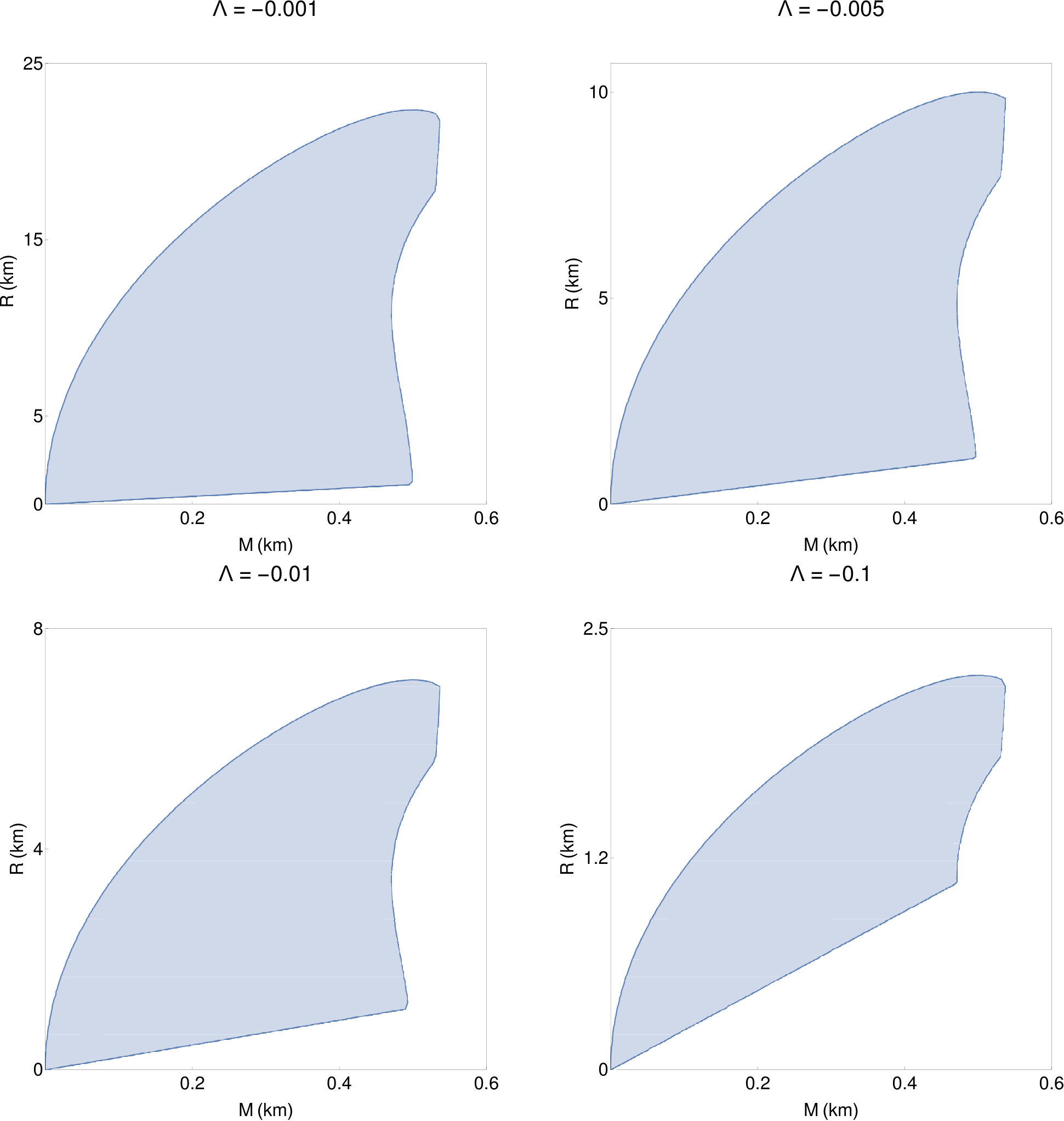
| Cosmological Constant | Mass in | Radius in |
| or | ||
| in | in | |
|---|---|---|
| 0.001 | ||
| 0.005 | ||
| 0.01 | ||
| -0.001 | 0.05 | |
| 0.1 | ||
| 0.5 | ||
| 0.53 | ||
| 0.001 | ||
| 0.005 | ||
| 0.01 | ||
| -0.005 | 0.05 | |
| 0.1 | ||
| 0.5 | ||
| 0.53 | ||
| 0.001 | ||
| 0.005 | ||
| 0.01 | ||
| -0.01 | 0.05 | |
| 0.1 | ||
| 0.5 | ||
| 0.53 | ||
| 0.001 | ||
| 0.005 | ||
| 0.01 | ||
| -0.1 | 0.05 | |
| 0.1 | ||
| 0.5 | ||
| 0.53 |
Some Physical Properties
Matching condition
The exterior spacetime of the static spherically symmetric compact object is assumed to be described by the BTZ metric as follow
| (15) |
The parameter is the conserved charge associated with asymptotic invariance under the time displacements. The continuity of and at surface and vanishing of normal pressure at surface yield
| (16) | |||||
| (17) | |||||
| (18) |
Behavior of energy density and pressure
For a physically acceptable model, energy density and radial pressure both should be monotonically decreasing function in and should be maximum at the centre. For our model, we have
| , |
| (24) |
At the centre (),
| (25) |
and
| (26) | |||||
| (27) |
The above eqn.(25-27) imply that central energy density and central pressure are maximum at the centre for any positive value of and .
The measure of anisotropy for our model is given by the expression
| (28) |
Based on the sign of the anisotropy parameter, the anisotropic force can be categorised in two: (i) the repulsive anisotropic force when i.e. and (ii) the attractive anisotropic force when i.e. [32]. This repulsiveness in anisotropic force enhances the stability of the star resulting in the star to be more compact than the isotropic one. [33, 34, 35]
Energy conditions
The energy conditions such as null energy condition (NEC), weak energy
condition (WEC), strong energy condition (SEC) and dominant energy condition
(DEC) should be satisfied at every point in the interior of the compact star
simultaneously. These energy conditions are as follows:
i) NEC: ;
ii) WEC: , ;
iii) SEC: , ;
iv) DEC: ;
Compactness and Surface Redshift
The compactness of the star is given by
| (29) |
The corresponding redshift is given by the expression
| (30) |
According to Buchdahl [36], the maximum value of i.e. is in dimension. The maximum allowed value of surface redshift [37] is in dimension. Cruz and Zanelli [38] have shown that Buchdahl’s theorem [36] remains to uphold also in dimensions. Therefore, we will use the same upper limit of the ratio of the mass to radius i.e. and the surface redshift in dimensions as we used in the case of dimension.
Generalized TOV Equation
The generalized TOV equation for anisotropic system is written as
| (31) |
This equation represents the equilibrium condition of the system under gravitational force (), hydrostatic force () and anisotropic force () as
| (32) |
where
| and |
The following form of the gravitational force (), hydrostatic force () and anisotropic force () for the Heintzmann line element is given below.
| (33) |
| (34) |
| (35) |
Conditions on the Metric parameters
Eqs. (25-27) indicate that both energy density and pressure are monotonically decreasing function and get maximized at the centre for any values of and in a positive domain. The central pressure and will be positive and real only when satisfying the conditions
| (36) |
The positivity of implies that
| (37) |
The dominating energy condition at the centre yields
| (38) |
The strong energy condition at the surface implies that
| (39) |
Example
PSR B0943+10
Yue et al., in the paper [3] showed that the small polar gap of PSR B0943+10 could be explained using Ruderman-Sutherland-type vacuum gap model if the pulsar has the mass and radii about and km respectively. We use our model for this pulsar and find out the useful parameters. If we use the mass of this pulsar as a only input parameter, then for , and our model predicts that the radii of this pulsar is in the range , and respectively. We enlist some parameters of this pulsar calculated using our model in table-3. One can observe (Fig.-2 and 3) that matter-energy density, radial pressure and transverse pressure are maximum at the centre and decreases monotonically towards the boundary. Also, one can see that radial pressure drops to zero at the boundary, while density does not. And although the energy density monotonically decreases, its value remains very high throughout the stellar system. Therefore, it may be justified to take these compact stars as strange stars where the surface density remains finite rather than the neutron stars for which the surface density vanishes at the boundary [39, 6, 40, 41, 42, 43]. Fig.4 suggests that the anisotropic force is attractive for our model. The attractiveness of the anisotropic force disallows the formation of massive compact star [32]. In other words, it allows the formation of the low mass compact star (strange star for our case). Fig.8 ensures that all the energy conditions are satisfied in our model. It is apparent from Fig.5 that the compactness, is an increasing function of the radial parameter and has maximum value below for all six cases. According to Buchdahl [36], the maximum value of i.e. is in dimension. Fig 7 shows that the value of surface gravitational red-shift has much less value than the maximum allowed value () [37] in dimension. Fig.9 shows that the gravitational force, the hydrostatic force and the anisotropic force are in equilibrium in the interior region of the star.
| Cosmological constant() | Radius (R) in km | Central energy density () in | Surface energy density () in | Central pressure () in | Compactness | Surface Redshift | A | a | c |
|---|---|---|---|---|---|---|---|---|---|
| 1 | 126.757 | 126.495 | 11.9498 | 0.029532 | 0.0309081 | 0.970019 | 0.00035401 | 108.462 | |
| -0.001 | 2.6 | 18.8449 | 18.6192 | 11.1187 | 0.011358 | 0.0115557 | 0.970027 | 0.00035257 | 13.7302 |
| 6.25 | 3.25651 | 3.22694 | 6.58000 | 0.004725 | 0.0047589 | 0.970285 | 0.00034472 | 0.00369 | |
| 0.7 | 259.054 | 257.788 | 58.6996 | 0.042189 | 0.0450611 | 0.970020 | 0.00176822 | 42.6728 | |
| -0.005 | 1.5 | 56.7741 | 55.7879 | 52.3773 | 0.019688 | 0.0202892 | 0.970041 | 0.00175728 | 7.14971 |
| 2.79 | 16.3438 | 16.1918 | 32.9976 | 0.010585 | 0.0107560 | 0.970283 | 0.00172375 | 0.01464 | |
| 0.5 | 507.770 | 505.241 | 117.327 | 0.059064 | 0.0648715 | 0.970020 | 0.00353631 | 41.7653 | |
| -0.01 | 1 | 127.657 | 125.606 | 106.541 | 0.029532 | 0.0309081 | 0.970037 | 0.00351765 | 8.38975 |
| 1.97 | 32.7843 | 32.4739 | 66.1483 | 0.014991 | 0.0153366 | 0.970281 | 0.00344777 | 0.02329 |
PSR J1640-4631
The X-ray pulsar PSR J1640-4631 high breaking index was explained by Chen [2] by considering the pulsar as a low mass neutron star having mass about . Chen [2] showed that the radius of this pulsar is about 29 km using the formula . Using our model, we get that the possible radius ranges for this pulsar are , and for , and respectively. In this paper, we estimate some parameters of this pulsar using our model presented in table-4. All the graphs related to this pulsar is very similar to the Pulsar PSR B0943+10 (we do not present graphs of this pulsar in this paper).
| Cosmological constant() | Radius (R) in km | Central energy density () in | Surface energy density () in | Central pressure () in | Compactness | Surface Redshift | A | a | c |
|---|---|---|---|---|---|---|---|---|---|
| 1 | 634.023 | 632.238 | 80.4903 | 0.147660 | 0.1912530 | 0.839452 | 0.00047258 | 414.783 | |
| -0.001 | 7 | 13.5744 | 12.3067 | 68.6351 | 0.021094 | 0.0217861 | 0.840080 | 0.00045207 | 6.86262 |
| 13.76 | 3.43523 | 3.25908 | 39.2116 | 0.010731 | 0.0109070 | 0.847190 | 0.00040117 | 0.00098 | |
| 1 | 637.489 | 628.800 | 397.307 | 0.147660 | 0.1912530 | 0.839459 | 0.00235400 | 81.7961 | |
| -0.005 | 3 | 73.7089 | 67.1735 | 347.918 | 0.049220 | 0.0531802 | 0.839985 | 0.00226856 | 7.63430 |
| 6.15 | 17.1999 | 16.3122 | 196.267 | 0.024010 | 0.0249106 | 0.847174 | 0.00200621 | 0.00448 | |
| 0.5 | 2541.37 | 2523.70 | 801.036 | 0.295320 | 0.5629580 | 0.839454 | 0.00471912 | 165.049 | |
| -0.01 | 2 | 165.243 | 151.671 | 707.789 | 0.073830 | 0.0831624 | 0.839876 | 0.00455780 | 8.81130 |
| 4.35 | 34.3760 | 32.6076 | 392.325 | 0.033945 | 0.0357772 | 0.847182 | 0.00401205 | 0.00273 |
1E 1207.4-5209
Xu in a paper [4] showed that the radio-quiet object 1E 1207.4-5209 could be a low mass bare strange star with mass and radii and km respectively. The radius ranges predicted by our model are , and for , and , respectively. Table-5 presents some parameters of this pulsar calculated using our model. Graphs related to this pulsar are similar to the pulsar PSR J1640-4631 (we do not show graphs of this pulsar in this paper).
| Cosmological constant() | Radius (R) in km | Central energy density () in | Surface energy density () in | Central pressure () in | Compactness | Surface Redshift | A | a | c |
|---|---|---|---|---|---|---|---|---|---|
| 0.5 | 25.3205 | 25.3093 | 0.53816 | 0.002952 | 0.0029651 | 0.998523 | 0.00033426 | 20.5610 | |
| -0.001 | 1 | 6.33220 | 6.32525 | 0.44135 | 0.001476 | 0.0014793 | 0.998523 | 0.00033410 | 2.89830 |
| 1.4 | 3.22967 | 3.22821 | 0.31754 | 0.001054 | 0.0010560 | 0.998524 | 0.00033388 | 0.01126 | |
| 0.1 | 632.903 | 632.841 | 2.82006 | 0.014760 | 0.0150950 | 0.998523 | 0.00167155 | 114.747 | |
| -0.005 | 0.3 | 70.3539 | 70.3034 | 2.56211 | 0.004921 | 0.0049573 | 0.998523 | 0.00167110 | 10.0970 |
| 0.627 | 16.1019 | 16.0948 | 1.58408 | 0.002354 | 0.0023624 | 0.998524 | 0.00166941 | 0.00261 | |
| 0.1 | 632.933 | 632.812 | 5.57552 | 0.014760 | 0.0150950 | 0.998523 | 0.00334298 | 55.8811 | |
| -0.01 | 0.2 | 158.292 | 158.188 | 5.18879 | 0.007381 | 0.0074637 | 0.998523 | 0.00334231 | 11.7326 |
| 0.44 | 32.6976 | 32.6817 | 3.20637 | 0.003354 | 0.0033715 | 0.998524 | 0.00333888 | 0.04858 |
Discussion and Conclusions
In this paper, we have presented a new model of the anisotropic low mass strange stars based on the Heintzmann ansatz in dimension. The attractive anisotropic force plays a significant role to bound the upper mass limit(which is comparatively low) of the strange star. The upper mass limit of the strange star for our model comes out as or for and for , where (see Eq-Appendix:A) depends on cosmological constant . So, we can say that "Strange stars, if they exist, can play an important role in the solution to the cosmological constant problem "[44, 45].
Table-1 presents the possible range of the cosmological constant , radius () and mass () of the low mass strange star. Fig-1 shows the accessible mass-radius region of our model. In this available region of the mass and radius, Buchdahl condition, all the energy conditions and other boundary conditions of the compact star are satisfied and the metric parameters , and are real and positive.
This model can be useful to analyze the low mass bare strange star [4]. In the paper [3], authors showed that PSR B0943+10 is a strange star having mass and radius km. Our model predict that a pulsar of mass has radii in between , and for , and respectively. Chen [2] argued that the high braking index of the PSR J1640-4631 can be explained by considering that PSR J1640-4631 is a low mass neutron star of mass . Using our model, we obtain that PSR J1640-4631 is a strange star because of non-vanishing surface energy density and get the radius range , and for , and , respectively. Xu [4] showed that 1E 1207.4â could have radius km and mass around . From our model, we get radius range , and for , and , respectively.
As the cosmological constant decreases, the central energy density and pressure and surface energy density increase for all three cases. For the fixed cosmological constant, the central energy density and pressure and surface energy density decrease as the radius increase in all three cases (see table:3-5). Fig.-9 indicates that the gravitational force and anisotropic force become identical while compactness is approaching the Buchdahl limit [36].
In this paper, we find the EoS having form , where is a dimensionless constant and has a dimension of is also a constant. Fig.-10 shows the relation between stellar interior radial pressure and energy density. Fig.-10 indicates that EoS found in our model is on the softer side.
It is to be mentioned here that we are comparing our results with the data from a dimensional object. Though for an observer in the or plane, the measured data will be approximately the same for both dimensions.
Acknowledgments
MM is thankful to CSIR (Grand No.-09/1157(0007)/ 2019-EMR-I) for providing financial support. NR is thankful to UGC MANF(MANF-2018-19-WES-96213) for providing financial support. MK is grateful to the Inter-University Centre for Astronomy and Astrophysics (IUCAA), Pune, India for providing Associateship programme under which a part of this work was carried out.
Appendix:A
| (41) |
| (42) |
| (43) |
| (44) |
| (45) |
| (46) |
| (47) |
| (48) |
| (49) |
References
- [1] H. Heintzmann. “New exact static solutions of einsteins field equations”. Zeitschrift für Physik, vol. 228, 489, 1969.
- [2] Chen, Wen-Cong. “High braking index pulsar psr j1640-4631: low-mass neutron star with a large inclination angle?”. A&A, vol. 593, L3, 2016.
- [3] Y. L. Yue, X. H. Cui and R. X. Xu. “Is PSR b0943+10 a low-mass quark star?”. Astrophys. J., vol. 649, no. 2, L95–L98, sep 2006.
- [4] R. X. Xu. “1E 1207.4-5209: a low-mass bare strange star?”. Mon. Not. R. Astron. Soc., vol. 356, no. 1, 359–370, 01 2005.
- [5] Ren-Xin Xu. “Low-mass bare strange stars”. Adv. Space Res., vol. 37, 1992–1995, 2006.
- [6] Charles Alcock, Edward Farhi and Angela Olinto. “Strange Stars”. Astrophys. J., vol. 310, 261, November 1986.
- [7] Ignazio Bombaci. “Observational evidence for strange matter in compact objects from the x-ray burster 4u 1820-30”. Phys. Rev. C, vol. 55, 1587–1590, Mar 1997.
- [8] X.-D. Li, I. Bombaci, Mira Dey, Jishnu Dey and E. P. J. van den Heuvel. “Is sax j1808.4-3658 a strange star?”. Phys. Rev. Lett., vol. 83, 3776–3779, Nov 1999.
- [9] Máximo Bañados, Claudio Teitelboim and Jorge Zanelli. “Black hole in three-dimensional spacetime”. Phys. Rev. Lett., vol. 69, 1849–1851, Sep 1992.
- [10] Norman Cruz and Jorge Zanelli. “Stellar equilibrium in 2+1 dimensions”. Class. Quantum. Grav., vol. 12, no. 4, 975–981, Apr 1995.
- [11] Alberto A. García and Cuauhtemoc Campuzano. “All static circularly symmetric perfect fluid solutions of gravity”. Phys. Rev. D, vol. 67, 064014, Mar 2003.
- [12] R. B. Mann and S. F. Ross. “Gravitationally collapsing dust in 2 + 1 dimensions”. Phys. Rev. D, vol. 47, 3319–3322, Apr 1993.
- [13] David Garfinkle. “Exact solution for (2+1)-dimensional critical collapse”. Phys. Rev. D, vol. 63, 044007, Jan 2001.
- [14] Paulo M Sá. “Polytropic stars in three-dimensional spacetime”. Phys. Lett. B, vol. 467, no. 1, 40–42, 1999.
- [15] Ranjan Sharma, Farook Rahaman and Indrani Karar. “A class of interior solutions corresponding to a (2+1)-dimensional asymptotically anti-de sitter spacetime”. Phys. Lett. B, vol. 704, no. 1, 1–4, 2011.
- [16] Farook Rahaman, Ayan Banerjee, Irina Radinschi, Sumita Banerjee and Soumendranath Ruz. “Singularity free stars in (2+1) dimensions”. nt. J Theor. Phys., vol. 52, no. 3, 932–945, Nov 2013.
- [17] Piyali Bhar, Farook Rahaman, Abdul Jawad and Sayeedul Islam. “Anisotropic charged fluids with Chaplygin equation of state in dimension”. Astrophys. Space Sci., vol. 360, no. 1, 32, 2015.
- [18] Ayan Banerjee, Farook Rahaman, Kanti Jotania, Ranjan Sharma and Indrani Karar. “Finch-Skea star in (2+1) dimensions”. Gen. Rel. Grav., vol. 45, 717–726, 2013.
- [19] Piyali Bhar, Farook Rahaman, Ritabrata Biswas and Hafiza Ismat Fatima. “Exact Solution of a (2+1)-Dimensional Anisotropic Star in Finch and Skea Spacetime”. Commun. Theor. Phys., vol. 62, no. 2, 221–226, 2014.
- [20] K. Schwarzschild. Preuss. Akad. Wiss., vol. 189, 424, 1916.
- [21] J.R. Oppenheimer and G.M. Volkoff. Phys. Rev., vol. 55, no. 374, 1939.
- [22] R.C. Tolman. Phys. Rev., vol. 55, no. 364, 1939.
- [23] S. K. Maurya, Y. K. Gupta, Saibal Ray and Baiju Dayanandan. “Anisotropic models for compact stars”. Eur. Phys. J. C, vol. 75, no. 5, 225, 2015.
- [24] S. K. Maurya, Ayan Banerjee, M. K. Jasim et al. “Anisotropic Compact stars in the Buchdahl model: A comprehensive study”. Phys. Rev. D, vol. 99, no. 4, 044029, 2019.
- [25] S. K. Maurya, Ayan Banerjee and Sudan Hansraj. “Role of pressure anisotropy on relativistic compact stars”. Phys. Rev. D, vol. 97, no. 4, 044022, 2018.
- [26] Y. K. Gupta and Sunil Kumar Maurya. “A class of charged analogues of Durgapal and Fuloria superdense star”. Astrophys. Space Sci., vol. 331, no. 1, 135–144, 2010.
- [27] S. K. Maurya, S. D. Maharaj and Debabrata Deb. “Generalized anisotropic models for conformal symmetry”. Eur. Phys. J. C, vol. 79, no. 2, 170, 2019.
- [28] S.K. Maurya and Y.K. Gupta. “A new family of polynomial solutions for charged fluid spheres”. Nonlinear Analysis: Real World Applications, vol. 13, no. 2, 677–685, 2012. [Online]. Available: https://www.sciencedirect.com/science/article/pii/S1468121811002355.
- [29] S. K. Maurya, S. D. Maharaj, Jitendra Kumar and Amit Kumar Prasad. “Effect of pressure anisotropy on Buchdahl-type relativistic compact stars”. Gen. Rel. Grav., vol. 51, no. 7, 86, 2019.
- [30] Krsna Dev and Marcelo Gleiser. “Anisotropic stars: Exact solutions”. Gen. Rel. Grav., vol. 34, 1793–1818, 2002.
- [31] Neeraj Pant, N. Pradhan and Mohammad Hassan Murad. “A Class of Super Dense Stars Models Using Charged Analogues of Hajj-Boutros Type Relativistic Fluid Solutions”. International Journal of Theoretical Physics, vol. 53, no. 11, 3958–3969, November 2014.
- [32] Mehedi Kalam, Farook Rahaman, Saibal Ray et al. “Anisotropic strange star with de sitter spacetime”. Eur. Phys. J. C, vol. 72, no. 12, 2248, Dec 2012.
- [33] M. K. Gokhroo and A. L. Mehra. “Anisotropic spheres with variable energy density in general relativity”. Gen. Rel. Grav., vol. 26, no. 1, 75–84, 1994.
- [34] Zacharias Roupas and Gamal G. L. Nashed. “Anisotropic neutron stars modelling: constraints in Krori–Barua spacetime”. Eur. Phys. J. C, vol. 80, no. 10, 905, 2020.
- [35] Sajahan Molla, Bidisha Ghosh and Mehedi Kalam. “Does dark matter admixed pulsar exist?”. Eur. Phys. J. Plus, vol. 135, no. 4, 362, 2020.
- [36] H. A. Buchdahl. “General relativistic fluid spheres”. Phys. Rev., vol. 116, 1027–1034, Nov 1959.
- [37] P. Haensel, J. P. Lasota and J. L. Zdunik. “Maximum redshift and minimum rotation period of neutron stars”. Nucl. Phys. B Proc. Suppl., vol. 80, 1110, 2000.
- [38] Norman Cruz and Jorge Zanelli. “Stellar equilibrium in (2+1)-dimensions”. Class. Quant. Grav., vol. 12, 975–982, 1995.
- [39] P. Haensel, J. L. Zdunik and R. Schaefer. “Strange quark stars”. Astron. Astrophys., vol. 160, no. 1, 121–128, May 1986.
- [40] Edward Farhi and R. L. Jaffe. “Strange matter”. Phys. Rev. D, vol. 30, 2379–2390, Dec 1984.
- [41] Mira Dey, Ignazio Bombaci, Jishnu Dey, Subharthi Ray and B.C. Samanta. “Strange stars with realistic quark vector interaction and phenomenological density-dependent scalar potential”. Phys. Lett. B, vol. 438, no. 1-2, 123–128, Oct 1998.
- [42] Matthias Herzog and Friedrich K. Röpke. “Three-dimensional hydrodynamic simulations of the combustion of a neutron star into a quark star”. Phys. Rev. D, vol. 84, 083002, Oct 2011. [Online]. Available: https://link.aps.org/doi/10.1103/PhysRevD.84.083002.
- [43] Norman K. Glendenning. Compact Stars:Nuclear Physics, Particle Physics and General Relativity. Springer-Verlag New York, 1997.
- [44] Cosimo Bambi. “Strange stars and the cosmological constant problem”. JCAP, vol. 06, 006, 2007.
- [45] Mehedi Kalam, Farook Rahaman, Sk. Monowar Hossein and Saibal Ray. “Central Density Dependent Anisotropic Compact Stars”. Eur. Phys. J. C, vol. 73, no. 4, 2409, 2013.