Python’s Lunches in Jackiw-Teitelboim gravity with matter
Dongsu Bak, Chanju Kim, Sang-Heon Yi, Junggi Yoon
a) Physics Department & Natural Science Research Institute
University of Seoul, Seoul 02504 KOREA
b) Department of Physics, Ewha Womans University, Seoul 03760 KOREA
c) Center for Quantum Spacetime & Physics Department, Sogang University, Seoul 04107 KOREA
d) Asia Pacific Center for Theoretical Physics, Pohang 37673 KOREA
e) Department of Physics, POSTECH, Pohang 37673 KOREA
f) School of Physics, Korea Institute for Advanced Study, Seoul 02455, Korea
(dsbak@uos.ac.kr, cjkim@ewha.ac.kr, shyi@sogang.ac.kr, junggi.yoon@apctp.org)
ABSTRACT
We study Python’s lunch geometries in the two-dimensional Jackiw-Teitelboim model coupled to a massless scalar field in the semiclassical limit. We show that all extrema including the minimal quantum extremal surface, bulges and appetizers lie inside the horizon. We obtain fully back-reacted general bulk solutions with a massless scalar field, which can be understood as deformations of black holes. The temperatures of the left/right black holes become in general different from each other. Moreover, in the presence of both state and source deformations at the same time, the asymptotic black hole spacetime is further excited from that of the vacuum solution. We provide information-theoretic interpretation of deformed geometries including Python’s lunches, minimal quantum extremal surface and appetizers according to the entanglement wedge reconstruction hypothesis. By considering the restricted circuit complexity associated with Python’s lunch geometries and the operator complexity of the Petz map reconstructing a code space operation, we show that the observational probability of Python’s lunch degrees of freedom from the boundary is exponentially suppressed. Thus, any bulk causality violation effects related with Python’s lunch degrees are suppressed nonperturbatively.
1 Introduction
The concept of entropy plays a fundamental role in various fields of theoretical physics. Especially in black hole physics, the entropy may pave a door-way to our understanding of quantum gravity. One of the well-established results in this regard is the Bekenstein-Hawking area formula [1, 2], which says that the black hole entropy is given by its horizon area divided by . Though this formula is regarded as a clue to the holographic nature of underlying degrees of freedom, it does not reveal their precise microscopic origin unfortunately. Based on the fact that the horizon works as a one-way door (not allowing anything to escape from a black hole classically), it has been proposed that the entropy may be understood as a fine-grained entanglement entropy between the interior and the exterior regions, divided by the black-hole horizon [3, 4].
As was argued by Page some time ago [5], the entanglement entropy of black holes should respect the unitary evolution of quantum mechanics and follow the so-called Page curve. This is incompatible with the result that the Hawking radiation is Planckian [6] while any correction to this result should be exponentially suppressed [7] and so an initially pure state is evolved into a mixed, as far as there is no remnant in the black hole evaporation process and the low energy effective field theory approach is valid. This conflict is one way to explain the information loss paradox in black hole physics, which is sharply reformulated as the firewall paradox [8]. For old black holes which have emitted more than half of their mass through the Hawking radiation, a newly generated Hawking radiation is entangled with both the early radiation and the behind horizon degrees of freedom, which is claimed to be in contradiction with the monogamy of the entanglement. Thus this conclusion must be evaded in some ways.
In this regard, there were rather crucial developments based on the so-called generalized entropy [1, 3]. One begins with a boundary region and its complement on a given boundary time slice. Along with a codimension two bulk surface that is homologous to and divides a bulk Cauchy slice ending on the boundary time slice into two regions, the generalized entropy can be defined, which consists of two contributions; One is given by the area of (divided by ) and the other by the entanglement entropy of bulk fields between the two regions divided by the surface . With this preliminary, the procedure to obtain the minimal quantum extremal surface (QESmin) goes as follows; First extremize spatially on a Cauchy slice specified in the above11 1 Usually, one picks all local minima of at this first stage. In this note, we instead include all extrema, which leads to the same QESmin at the end of the day., and then maximize among all possible choices of Cauchy slices for the given boundary, which leads to a set of extremal surfaces. Among these extremal surfaces, we choose the global minimum, which singles out the desired QESmin [9, 10, 11]. This can be thought of as a generalization of the Ryu-Takayanagi surface [12, 13, 14], which has been explored in various contexts as a holographic realization of the entanglement entropy of a boundary region. The generalized entropy in some examples can be computed explicitly, explains the Page curve, and evades the firewall through some further identification: entanglement wedge island. It has been argued under the central dogma that some part of black hole interior degrees of freedom associated with the island are actually belonging to the radiation (see for a review [15]); An outside observer acting on the radiation only may in principle probe the island degrees of freedom directly, which appears rather bizarre as they are at least shielded by the horizon!
Python’s lunches are closely related to the island wedges just mentioned [16]. In general, among all extremal surfaces, one may have a local maximum placed between two saddle surfaces. Such a local maximal surface is called a bulge surface whereas the remaining saddle surfaces except the QESmin are called appetizers. Python’s lunch geometries are involving at least one bulge and one appetizer. In this note we would like to understand the nature of Python’s lunch degrees of freedom. In order to understand them, one may borrow various concepts and results from quantum information theory and its realization in the context of the AdS/CFT correspondence. These include the entanglement wedge reconstruction, quantum error correcting codes, the holographic tensor network, circuit complexity and so on [17, 18, 19, 20, 21, 22, 23, 24, 25].
In particular, quantum complexity plays an essential role in our understanding of the Python’s lunch degrees of freedom. It has been known that there are two versions of complexity. One is the unrestricted version of complexity associated with an observer who may access the entire quantum system of interest. For instance, in two-sided eternal black holes, probed by an observer who may access both boundaries, the unrestricted complexity of the thermo-field-double (TFD) state under time evolution is holographically related to the time-dependent expansion of the black hole interior region [26, 27, 28]. In the bulk picture, this complexity may be identified using the volume/action conjecture. The other is the restricted complexity where an associated observer can access only part of the underlying quantum system. A rather well-known example is the computational complexity arising in decoding information out of Hawking radiation [29, 30]. In this note, we shall be mainly concerned about the restricted complexity in order to understand the nature of Python’s lunch degrees of freedom.
In this note we focus on the two-dimensional Jackiw-Teitelboim (JT) model [31, 32] coupled to massless scalar fields in its semiclassical limit. We shall identify all possible deformations of black hole solutions which may involve Python’s lunch geometries. It turns out that, in the semiclassical limit, all extrema including QESmin, bulges and appetizers lie inside the horizon, which basically follows from the null energy condition (NEC). This deformed two-sided black hole spacetime is to be divided into left and right wedges that share QESmin as a separating surface (point in 2d). Under the entanglement wedge reconstruction hypothesis, all local bulk operations within the left/right wedge can be reconstructed out of the corresponding operations on the left/right boundary Hilbert space. For definiteness, let us choose the right wedge and consider a minimal Python’s lunch lying behind the horizon of the right side. Within this, there are specific local bulk degrees of freedom that are genuinely associated with the Python’s lunch (-degrees in short) and the remaining local bulk degrees of freedom in the region outside the appetizer (-degrees in short). The combined bulk Hilbert space should be mapped to the full boundary Hilbert space of the right side. We shall review the restricted complexity of Python’s lunch geometries that is exponential in their number of degrees. We shall also review the operational complexity of the Petz map by which one reconstructs code space operations acting on the bulk Python’s lunch Hilbert space out of -Hilbert space of a one-sided boundary. Based on these, we shall argue that observational probability of Python’s lunch degrees of freedom by some boundary experiment acting on -Hilbert space is exponentially suppressed. Thus, any bulk causality violation effects related with Python’s lunch degrees are suppressed nonperturbatively.
This paper is organized as follows. In section 2 our setup is given with the emphasis on the two-sided black hole solutions. In section 3 we provide a generic deformation of a scalar field solving the equation of motion. For concreteness we consider the massless scalar field only. We also present the general profiles of the dilaton field. In section 4 it is shown that the deformation of the dilaton field solution can be understood as the deformation of black holes. Exploring the effects of the scalar field deformation on the black holes, we show that the temperatures of two-sided black holes can be asymmetric between the left and right sides. The end points of the horizon are also studied and it is shown that the traversable wormholes cannot be formed by our deformation. We show that QESmin, Python’s lunches, and appetizers reside behind the horizon in our semiclassical setup. In section 5 we provide some geometric interpretation of our results including python’s lunch, appetizer, QESmin, and the entanglement wedge reconstruction hypothesis. In section 6, based on our study, we give some reviews and comments on the related aspects of the complexity, the information reconstruction from the one-sided boundary state, and the interaction among the degrees of freedom including Python’s lunch degrees of freedom. In the final section, we summarize our results and provide some future directions.
2 Two-dimensional dilaton gravity
Our basic setup is a 2d dilaton gravity known as the JT model coupled to a matter field [31, 32, 33], whose action is given by
| (2.1) |
where
| (2.2) |
For a well-defined variational principle, we need to add a surface term
| (2.3) |
to the above where and denote the induced metric and the extrinsic curvature on the boundary which is taken to be timelike.
The equations of motion read
| (2.4) | ||||
| (2.5) | ||||
| (2.6) |
where
| (2.7) |
The global AdS2 space corresponds to the metric solution to the equations of motion, whose form is given by
| (2.8) |
where the spatial coordinate is ranged over . The dilaton field configuration for the most general vacuum black hole solution reads
| (2.9) |
By the coordinate transformation
| (2.10) |
one is led to the corresponding AdS black hole metric
| (2.11) |
with
| (2.12) |
In general, this black hole metric describes only the Rindler wedge of two-sided AdS black holes. The location of singularity is defined by the curve in the above dilaton field, and might be viewed as characterizing the size of transverse space from the viewpoint of dimensional reduction from higher dimensions22 2 For example, the dimensional reduction of 4d near-extremal black holes has been investigated in [34], which leads to our JT gravity with matter fields. This reduction is well controlled once [35, 34] where denotes the value of the dilaton at asymptotic cut-off trajectories introduced below. Of course, for the well-defined nearly AdS2 dynamics, we also require . With these conditions, our solutions below can be consistently embedded into the 4d theory. [33]. In this left/right symmetric two-sided black hole, one can see that the Hawking temperature, the entropy and energy are given by
| (2.13) |
where and denote the ground state entropy and the specific heat, respectively. In general, these physical quantities may be different for left/right Rindler wedges in deformed two-sided black holes. In the next sections we consider general deformations with a scalar field starting from the left-right symmetric black hole configuration with and . We find that the above left-right thermodynamic quantities indeed become different from each other in general with a nontrivial matter field profile.
Before going ahead, let us recall a simple left-right asymmetrically deformed configuration with a massless scalar, known as the eternal Janus deformation [36, 37]. In this case, the black hole temperature and the dilaton field configuration are left-right symmetric under the exchange , but the matter field configuration is not left-right symmetric. This simple Janus solution is given by
| (2.14) |
The Penrose diagram of this configuration with contribution is given in Figure 1.
Now, we would like to present the matter field solution to the equations of motion in (2.5), which is given by
| (2.15) |
where
| (2.16) |
and denotes the Gegenbauer polynomial. Here, the parameter is related to the mass of the scalar field as
| (2.17) |
The AdS/CFT dictionary tells us that the bulk matter field with mass , when , is dual to a scalar primary operator , where its dimension is given by the larger one of as
| (2.18) |
The deformation by the scalar field with corresponds to a state deformation of the dual field theory, while the other deformation with does to a source deformation. When scalar field mass squared is negative but above the Breitenlohner-Freedman bound [38], which is given by in our case, both possibilities of operator dimensions may be realized as
| (2.19) |
In this paper, we focus on the bulk classical configuration by ignoring the loop corrections. This limited consideration may be justified by keeping the Newton constant very small and by introducing a controllable number of identical scalar fields, say , without self-interactions [39]. With the combination fixed, one finds that any loop corrections are suppressed as where is counting the number of loops involved.
3 General deformations with a massless scalar field
From now on, we shall focus on turning on a massless scalar field that is dual to a scalar operator of dimension . In this section we are mainly interested in fully back-reacted bulk solutions with the massless scalar field. Based on these solutions, we shall identify rather general Python’s lunch geometries that are arising if certain parameter conditions are met. For this, we note that the metric solution to the equation (2.4) remains the same while the bulk scalar equation (2.5) (with ) may be solved explicitly by
| (3.1) |
where
| (3.2) |
and
| (3.3) |
This describes a full-set of classical solutions of the scalar equation in the ambient AdS2 space with the global coordinates. The bulk solution with corresponds to the state deformation of the left/right boundary quantum system without deforming our boundary theories33 3 One may specify the well-known correspondence between JT gravity and SYK system. But such detailed specification does not play much role in our description of this paper.; This leads to a nontrivial vev of the dimension-one operator in the boundary theory. On the other hand, the bulk solution with corresponds to the source deformation of boundary Lagrangian by where denotes the time coordinate of our left/right boundary system going upward direction44 4 Note that the left-right values of vev and source are not independent since our undeformed bulk configuration corresponds to the TFD state in the boundary..
In our JT model, the metric remains to be AdS2 with an arbitrary matter perturbation, as mentioned previously. For the dilaton field, we shall consider deformations from the vacuum solution
| (3.4) |
which describes a two-sided black hole with temperature . When the matter field is turned on, the two-sided black hole will be perturbed in general left-right asymmetrically as we shall analyze in detail in later sections.
Considering first the state perturbation with , the dilaton solution becomes
| (3.5) |
where
| (3.6) |
and
| (3.7) |
with . The remaining off-diagonal contribution is given by
| (3.8) |
which satisfies . The terms in (3.6) and (3) can be obtained by taking and up to some homogeneous terms.
For the sake of an illustration, we here present the gravity solution with where . The corresponding dilaton solution in this case becomes
| (3.9) |
where the three diagonal terms are given by
| (3.10) | ||||
The remaining off-diagonal terms can be organized as
Note that the left and right boundaries of our AdS2 spacetime are located respectively at . In these asymptotic regions, the dilaton solution behaves as
| (3.11) |
Indeed one may explicitly check this behavior for and with nonvanishing contributions to . The remaining term as we approach the left/right boundaries does not contribute to . This trend continues with the general mode-solution for arbitrary and . Namely, the contributions from and are nonvanishing. On the other hand, as and, consequently, has no contribution to .
We here also present a general solution for the source deformation with . The corresponding dilaton solution can be obtained as
| (3.12) |
where
| (3.13) |
and
| (3.14) |
with . The remaining off-diagonal contribution is given by
| (3.15) |
which satisfies . The contributions in (3.13) and (3) can be obtained by taking and up to some homogeneous terms.
We note that the dilaton solution is independent of since its contribution to the energy momentum tensor vanishes. Hence we shall set to zero for simplicity in our presentation. Also one finds that the general structure of is similar to that of which is from the state deformation. Indeed one finds that the relation
| (3.16) |
works with . Hence in our study of Python’s lunch geometries in Sec. 5, we will focus on the case of the state deformation (or the source deformation alternatively) unless both are turned on at the same time.
Finally one may also consider the full general deformation with . Then the corresponding dilaton solution may be obtained as
| (3.17) |
where
| (3.18) |
and
| (3.19) | ||||
| (3.20) |
with .
The remaining term is given by
| (3.21) |
Again the contributions in (3) and (3) can be obtained by taking , and up to some homogeneous terms.
In the following sections, we shall analyze the asymptotic form of the above solutions in detail. The resulting left/right black holes are deformed in general. For instance, the Hawking temperatures of the left/right black holes become in general different from each other. Especially when both state and source deformations are present at the same time, the asymptotic black hole spacetime is further excited rather nontrivially.
Finally one may also consider chiral deformations for which either and . (In our classical case with the massless scalar field, automatically.) This type of deformations is realized by choosing and . Then the scalar field becomes
| (3.22) |
which gives us with , respectively. Here, we introduced . In these coordinates, the equation of motion for the dilaton involving becomes
| (3.23) |
Thus one may show that the dilaton field can be written in the form of
| (3.24) |
for , respectively.
4 Deformations of two-sided black holes
In this section, we shall analyze the resulting deformation of the two-sided black hole spacetime including the horizon structure and the late-time temperature of the black hole system.
Physical properties of the deformed system can be obtained by studying the asymptotic behavior of the dilaton solution. We shall see that, when only one kind of deformation of the two in (3.1) is turned on, the asymptotic behavior of the dilaton reduces to the form of the vacuum solution (2.9) with deformed constants. In general the Hawking temperatures of the left/right black holes changes differently from each other. Although there can be many nontrivial Python’s lunches developed in the bulk, the boundary dynamics will be that of simply deformed black holes with corresponding modifications in the cut-off trajectory and does not directly capture the effect of the Python’s lunches. In the presence of both the state deformation and the source deformation, the asymptotic behavior of the dilaton turns out to be more complicated than the vacuum solution (2.9). This would be then reflected in the boundary dynamics as a new term in the boundary action as well as more complicated trajectories.
To see first the causal structure of the solution (3.12), let us study its asymptotic behavior as . Note that, as ,
while all the remaining of are . We shall also introduce by the rescaling . The dilaton in asymptotic regions can then be written in the form of (3.11) with
| (4.1) |
Here and below the upper/lower sign inside parenthesis is for the left/right boundary region respectively.
As was noted previously [35], the reparameterization can be fixed by the prescription of the dilaton cutoff
| (4.2) |
treating as a radial coordinate in the asymptotic region. This will fix the asymptotic left/right cutoff trajectory . For simplicity below, we shall frequently drop the index and since the left and right asymptotic regions can be treated in the same way. Through the asymptotic form of the dilaton field in (3.11), the trajectory is then given by
| (4.3) |
The reparameterization on this trajectory enables us to express in terms of the boundary time . Namely, from the prescription in the metric in (2.8), we have
| (4.4) |
This leads to
| (4.5) |
We arrange as in the form of
| (4.6) |
where
| (4.7) |
For the asymptotic region to be well-defined, and is required. Then the reparameterization is solved by
| (4.8) |
where . Since is the boundary time coordinate of the cutoff trajectory in the Rindler wedge in (2.11), the late-time temperature of the deformed system becomes
| (4.9) |
One further find that the future/past infinity of the Rindler wedge is at
| (4.10) |
which can also be obtained from . Then the L/R future horizons are described by straight lines
| (4.11) |
while the L/R past horizons are by
| (4.12) |
The corresponding Penrose diagram is depicted in Figure 2.
Note that in this figure the end points of the future/past horizon are shifted from to values with . This can be seen from
| (4.13) |
where . Since
| (4.14) |
the numerator of (4.13) is positive semidefinite, which proves .
In case of the source deformations where the dilaton is given by (3.17), the functional form of each mode is essentially the same as that of the state deformation and hence we get the same results. However, for the full general deformations (3.1) including both state as well as source deformations, we obtain rather different behaviors due to the cross terms in (3.17). To see this, let us first consider the simplest case where both the state and the source deformations are turned on,
| (4.15) |
with the corresponding dilation solution
| (4.16) |
As , behaves as in (3.11) with
| (4.17) |
where . Note that the cross term in contains a linear term in which cannot be obtained as a function of in a closed form. For small deformations, one can still compute future/past infinities at which vanishes. The results are
| (4.18) |
where
| (4.19) |
Here the ellipses are quartic order terms in and and the upper/lower sign refers to the left/right boundary respectively as before. Note that is not negative/positive definite. In other words, can be larger than when both the state and the source are deformed together, in contrast with the previous cases where only one kind of deformation is turned on. Nevertheless, for this particular deformation with the lowest modes, the difference of the future infinity and the past infinity is still less than or equal to , i.e.,
| (4.20) |
Then the difference becomes smaller by the perturbation, although the overall spacetime is slightly shifted either upward or downward.
From (4), one can also compare shifted values in other boundaries. Suppose for instance that . (The other case can be treated in a similar manner.) Assuming , this happens only when
| (4.21) |
Then it is not difficult to see that the following relation holds
| (4.22) |
Therefore although the position of the future infinity at the right boundary is shifted slightly upward, the other three positions are also moved enough to compensate for such shift. In particular, implies that the causal structure is not of the type of traversable wormholes, as it should be for classical perturbations.
Having seen what happens when both the state and the source deformations are turned on, let us now consider the most general deformation (3.1). Denote
| (4.23) |
where is given by
| (4.24) |
with
| (4.25) |
Then
| (4.26) |
where ellipsis is of quartic or higher order in ’s and ’s. Nonvanishing contributions from the cross term are
| (4.27) |
and for and even,
| (4.28) |
Collecting terms from , and , we have
| (4.29) | ||||
We can explicitly diagonalize (4.29) for some finite number of deformations. If for , we find that (4.29) is negative semidefinite. If higher modes are present, however, it turns out that (4.29) can be positive because of the cross terms. In other words, if high enough modes of both state and source deformations are turned on at the same time, the difference between the future infinity and the past infinity in one side can be larger than . Since in the presence of only one type of deformations as seen above, this result is due to the interaction of both deformations for which the asymptotic black hole spacetime is nontrivially excited from the vacuum solution. Also, the trajectories of the boundary dynamics would be deformed accordingly.
On the other hand, the difference of the future infinity of one side and the past infinity of the other side must still be less than or equal to for arbitrary deformations, since traversable wormholes should not be formed. Indeed, we find that
| (4.30) |
where can be written in a manifestly negative semidefinite form,
| (4.31) | ||||
Since the general dilaton solution (3.17) is an infinite series of trigonometric functions with arbitrary coefficients, one may wonder if the extremum points of can exist anywhere in the spacetime. We shall argue, however, that classically they should reside behind the horizon thanks to the NEC. Let us focus on the right Rindler wedge for definiteness. In terms of the affine parameter for a fixed ,
| (4.32) |
the equation of motion (3.23) in null coordinates can be written as
| (4.33) |
which is the two-dimensional analogue of the Raychaudhuri equation. Here, plays the role of the expansion of the null geodesic congruence. Now, the positive NEC () implies
| (4.34) |
which shows us that null rays from the extremal point of , defined by , should be met with a singularity within a finite affine parameter and so the extremal points should reside behind the horizon. Note that this is nothing but a two-dimensional version of the famous singularity theorem or the focusing argument [40, 41, 42].
In case of the chiral deformations (3.22), the situation is rather simple. For definiteness, let us choose the upper sign in (3.22) which corresponds to . Then there are only ingoing/outgoing modes in the right/left sides and we expect that the future/past horizons of the right/left black holes would be deformed to outwards/inwards so that they do not meet at one point. On the other hand, the other side of the horizons, namely the past/future horizons of the right/left black holes would be still connected as a single straight line. See Figure 3. This can easily be seen from the general form of the dilaton solution (3.24). Note that at the horizon we would have , where is the relevant affine parameter. It implies the equation which is independent of . Then in the spacetime under consideration where the horizon is unique at each asymptotic region, the solution should define a unique straight-line throughout the spacetime. In other words, it represents the past/future horizons on the right/left sides connected as a single straight line as expected.
We now show that the extremal point should be unique and lie on the horizon for chiral deformations. First, it is evident that results in which is nothing but the defining equation of the horizon . The other condition for the extremal point gives
| (4.35) |
which has a unique solution on the horizon ,
| (4.36) |
which completes the proof. Note in particular that there cannot be a Python’s lunch at least classically for chiral deformations.
5 Python’s lunch geometries
In this section, we discuss Python’s lunch geometries formed by the general deformations. Let us first consider the Janus deformation (2.14) to identify a Python’s lunch in the simplest setup. Since is the only -dependent term in the dilaton configuration (2.14), we should consider the slice to find any extremum point. At , the dilaton field can be written as
| (5.1) |
where we set in this section. Then as ,
| (5.2) |
which requires . For , becomes
| (5.3) |
where . It is clear that, for small positive , is a maximum point of . The QESmin is the minimum point of which occurs at with
| (5.4) |
Therefore, for , a bulge is formed at and QESmin is located at . The difference of the two dilaton values is
| (5.5) |
We draw the dilaton field under the Janus deformation in Figure 4.
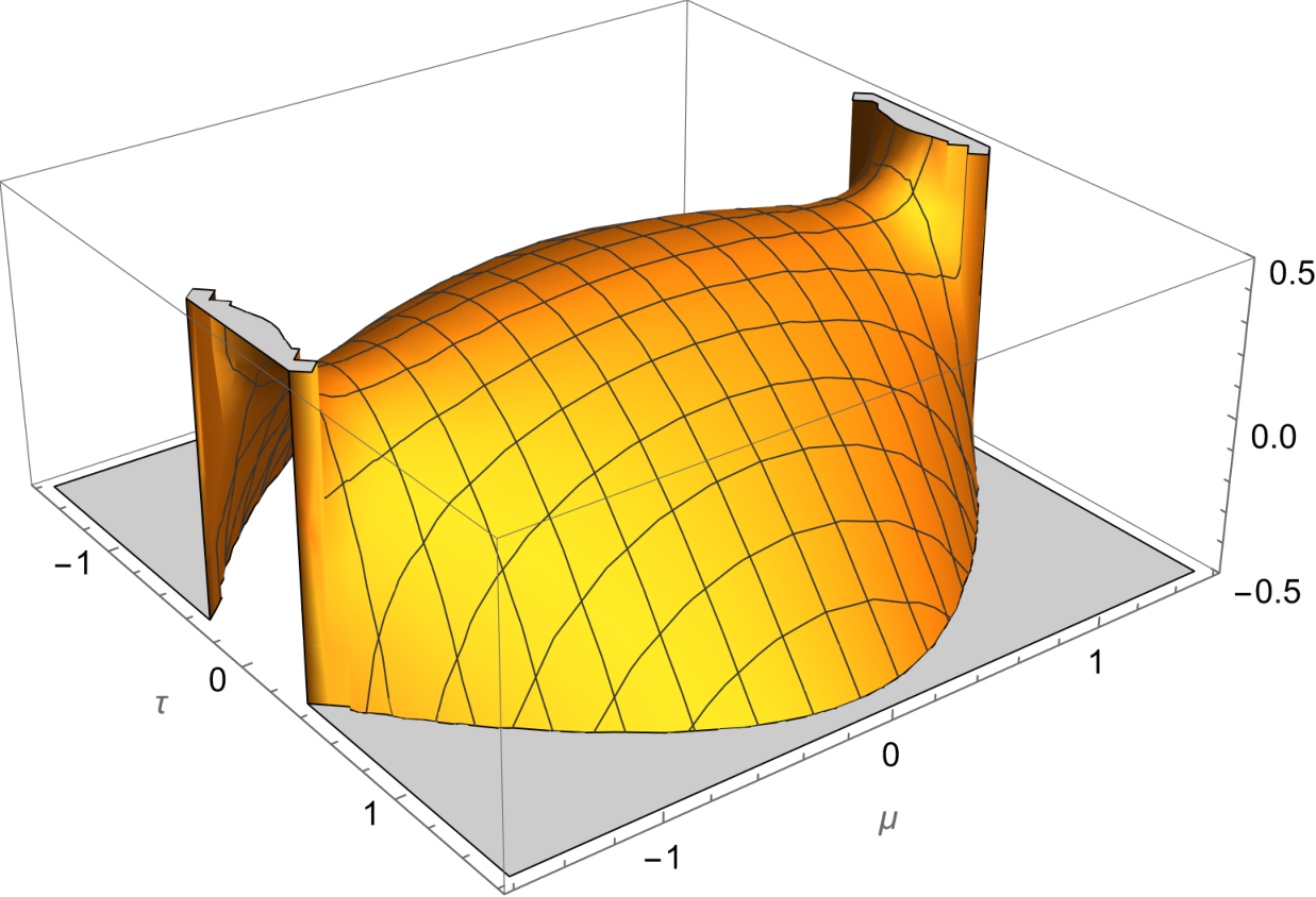
Now we look into more general deformations analyzed in section 3. For the lowest-mode state deformation , the dilaton solution is given by (3.9) and (3). Choosing and such that , the dilaton is positive definite and has a maximum at and hence a Python’s lunch geometry is formed around the origin, as depicted in Figure 5. For , the QESmin occurs at while, as increases, its position moves towards .
So far, we have considered left-right symmetric configurations. The QESmin in this case is located at two places, one in region and the other in region, respectively, since the dilaton fields are even functions of . If we turn on several modes at the same time, the dilaton has cross terms which can be odd in as seen in (3). Then the degeneracy is broken and we have only one QESmin at either left or right region. This is illustrated in Figure 5, where the first and the second modes are turned on at the same time, , and the dilaton has a cross term in (3) which is an odd function of . In the figure, there are three extrema which can be identified as the QESmin, a bulge and an appetizer, respectively from the left.
Geometries with two Python’s lunches can be obtained by turning on three lowest modes (3.9). See Figure 5. By now, it should be clear that one can generate very complicated geometries by suitably turning on higher modes. Figure 5 is an example of this kind, where two modes are turned on with and . In these figures, phases ’s are set to be so that the dilaton configuration is symmetric under the time reversal which guarantees that slice has extrema. One can consider, however, more general configurations by choosing other values for .
In Figure 6, we draw a typical dilaton configuration and the corresponding Penrose diagram of deformed two-sided black hole spacetime. There is a unique QESmin at the true minimum of the dilaton. At the local maxima, we have three bulges denoted by , and , respectively. There are also three appetizers denoted by , and , respectively, and they correspond to local minima. Superscript L and R refer to the relative positions with respect to the QESmin. In the Penrose diagram, horizons are drawn in black lines. Note that all the extrema are behind the horizons as argued in section 4. The spacetime is divided into the left and the right wedges with QESmin as a separating point, as drawn in red lines. Then, according to the entanglement wedge reconstruction hypothesis, all local bulk operations in each wedge should be able to be reconstructed in the corresponding boundaries as operations on each boundary Hilbert space. In the left wedge having an appetizer and a bulge , the local bulk degrees of freedom in the leftmost wedge outside should admit a simple boundary reconstruction based on the HKLL reconstruction [44, 45], including those between the horizon and the appetizer [46]. The degrees of freedom associated with Python’s lunch with is discussed in section 6. In the right wedge, there are two Python’s lunch geometries with bulges and respectively, which are separated by the appetizer . The local bulk degrees of freedom in the right wedge are then associated with one of the Python’s lunches or the rightmost wedge outside the appetizer . Note that the generalized entropy of the first bulge is larger than that of the second bulge .
As we have demonstrated above, extrema of the dilaton can change depending on matter perturbations. Suppose that with a suitable perturbation, the dilaton value at, for example, is lowered and eventually gets smaller than the dilaton value at the current QESmin. Then the position of the QESmin would make a transition from the current QESmin to . Accordingly, the degrees of freedom associated with would belong to the left wedge of the new QESmin. In this case, those degrees would no longer be reconstructed from the right boundary according to the entanglement wedge hypothesis. Instead, it would be reconstructed from the left boundary.
6 Complexity, reconstruction and ghostly interactions
In this section, we would like to first briefly review the restricted circuit complexity associated with Python’s lunch geometries [16, 42]. For definiteness, we limit our attention to the right wedge that lies on the right side of the true QESmin as illustrated in Figure 7 and take, for simplicity, a basic lunch with one bulge and one appetizer 55 5 At each point, the associated entropy in the classical regime is given by the formula in our JT model.. We consider an isometry map from a state with basis defined on the QESmin to the appetizer state with basis . This requires which follows from the fact that the QESmin is the minimum of all extremal surfaces. The bulge Hilbert space can be written as where with basis is associated with the Python’s lunch degrees of freedom. The number of its associated qubits is identified as
| (6.1) |
where is the dimension of the Hilbert space with . The map is realized as follows. In the tensor network picture of the bulk [47] illustrated in Figure 7, one has an isometry from to but the map from to cannot be isometric. Instead it is given by the adjoint of an isometry and hence constructing the map becomes nontrivial. Namely adding ancilla qubits with , one may represent the map by
| (6.2) |
In Figure 7, the orange colored dots between the QESmin and the bulge represent the ancilla qubits. The black dots the represent required post-selected qubits, which are identified as the Python’s lunch degrees of freedom in the above. Since the postselection is nonunitary, the trick is to use the unitary operations of Grover search algorithm [48, 49] whose the required number of simple operation is given by the order of . This leads to the circuit complexity of the Python’s lunch
| (6.3) |
as was shown in [16].
For a general Python’s lunch, we again consider a general Python’s lunch geometry in the right wedge which involves bulges and appetizers with . In [42], it was shown that the associated circuit complexity is given by
| (6.4) |
where defined only for . We shall call as and the relevant bulge and appetizer of this maximum as maximum bulge and appetizer respectively.
Next we review the Petz map reconstruction of code space operation from the boundary theory and its operational complexity in the presence of the Python’s lunch degrees of freedom [50]. For this purpose, we consider a code space state of (with a basis that is embedded into the full Hilbert space of on the right multiplied with the Hilbert space on the left where the left and the right side are entangled through the QESmin. Specifically this embedding defines an isometry given by
| (6.5) |
where
| (6.6) |
This requires some clarifications; First the unitary operator is introduced in such a way that
| (6.7) |
where represents a specific ancilla qubit state and their Hilbert space basis will be denoted by . The number of total ancilla qubits is determined such that
| (6.8) |
Again the -qubits represent the Python’s lunch degrees of freedom, whose number of qubits is given by (6.1) as before. On the other hand, the -qubits are for the degrees of freedom with relatively low-complexity, which lie on and outside the outermost appetizer extremal surface. We take their Hilbert space dimension to be large enough such that
| (6.9) |
The -qubits represent the QESmin degrees of freedom, which are responsible for the left-right entanglement in the state . We also introduce a further separation of the ancilla qubits into two parts as indicated by and their basis by with the relation . With help of this setup, we define fully by
| (6.10) |
without the restriction of the specific ancilla qubit state. Now, the operator is completely defined as a unitary operator acting on . The Python’s lunch state is not available from the viewpoint of a right-side observer who can perform only relatively low-complexity operations. Thus from the viewpoint of this observer, one is tracing over the space in the construction of the Petz map below.
Finally when the unitary matrix is assumed to be random enough [50], the operator defined by
| (6.11) |
becomes a unitary operator that is acting on ignoring any negligibly small corrections in all practical senses. Namely the set forms an orthonormal basis of again ignoring any negligibly small corrections. Note also that depends on a specific , which indicates the state dependence in the above construction of .
The Petz map of our interest can reconstruct a code space operation , which may be understood as a black hole interior operator in the Hayden-Preskill protocol [29],
| (6.12) |
from the state by some operation within the Hilbert space alone. The map is realized by [24, 25]
| (6.13) |
with
| (6.14) |
One then finds that, for a specific inherited from ,
| (6.15) |
It is clear that the reconstruction is made by the operation within the space of . This map may be rewritten as
| (6.16) |
As was already shown, may be expressed in terms of matrix with some postselection, which is illustrated in Figure 8. It is also clear that the action involves a Python’s lunch configuration of extra qubits. In addition, its realization by requires the postselection to the state as illustrated by dotted legs in the Figure 8. Hence we conclude that the operator complexity of the Petz map becomes
| (6.17) |
which was first shown in [50].
Finally we would like to discuss observational difficulties in detecting the Python’s lunch degrees of freedom (see [51] for some related discussions). In our setup, a computationally bounded observer performs relatively simple operations that are limited to the Hilbert space introduced above. Of course, such probe of the Python’s lunch degrees of freedom will not be feasible. For instance, the bulk causality, in the classical regime, forbids the boundary observer to detect these degrees of freedom since they lie behind the horizon. Hence any of these probes ought to be based on certain quantum effects such as Hawking radiation. Below we shall show that their observational signature is suppressed exponentially in and, hence, nonperturbative.
As before, we use the isometry map in (6.5) where we take an empty code space, i.e. . Then the state in (6.6) may be rewritten as
| (6.18) |
where the state reads66 6 Strictly speaking, the case of was not included in the consideration of [50].
| (6.19) |
with the orthonormality
| (6.20) |
One may view the state as the maximally-entangled counterpart of the Python’s lunch state .
We would like to probe the state by a certain interaction amplitude that induces a transition from to with an amplitude (). This amplitude is assumed to be . We may introduce such amplitudes to confirm the state but let us drop the index below for the simplicity of presentation.
The transition amplitude from to then becomes
| (6.21) |
whose magnitude squared may be estimated as
| (6.22) |
To show this, we note that . As was just shown, the complexity of the unitary (or equivalently ) is given by . This implies that the state is spreading nearly uniformly over some -number of its basis states. Therefore we conclude that
| (6.23) |
Thus the amplitude is indeed exponentially suppressed in and the state cannot be detected through any perturbative interactions on the boundary. Namely the Python’s lunch degrees lie within the almost completely dark sector of the system. This is also consistent with the claim [52] that any ghost operators acting on the Python’s lunch Hilbert space nearly commute with any operation on applied by any computationally bounded observer. As in [52], our argument for the above exponential suppression involves a state dependence since the construction depends on and .
Finally we would like to comment on the degrees of freedom lying outside the outermost appetizer but still inside the horizon. The restricted complexity associated with these degrees of freedom may be estimated as the volume of the region divided by following for instance the volume conjecture [26] of holographic complexity. Repeating a similar reasoning as in the above, the observational probability through some boundary interactions may be estimated as
| (6.24) |
Hence these degrees of freedom can be probed perturbatively by appropriate boundary experiments. This is consistent with the fact that, in evaporating black holes, information on such degrees of freedom may be transferred to their Hawking radiation after their Page time, which is a semiclassical effect of . This is also consistent with the observation [46] that the reconstruction of such degrees of freedom may be achieved with relatively simple boundary operations.
7 Conclusions
In this work, we have presented the deformation of the two-dimensional black hole by a massless scalar field which realizes Python’s lunch geometries. First, we have studied the deformation of JT gravity by the massless scalar field. With general source and state deformations, a full general solution of the dilaton has been derived. And then, from the asymptotic behavior of the dilaton solution, we have identified the locations of the deformed horizons and the future/past infinities. Here, we have shown that the difference of the future infinity of one side and the past infinity of the other side is less than in the global time coordinate, and from the NEC we have also demonstrated that any extremal points of the dilaton are located behind of the horizon. In addition, we have calculated the extremal points of the deformed dilaton solution to find the QESmin, Python’s lunches and appetizers. We have shown that the position and the number of Python’s lunches and appetizers can vary drastically by tuning the deformation parameters. Finally, we have discussed the restricted complexity of the general Python’s lunches and the reconstruction of a code space operator via a Petz map. We have explained why it is difficult to probe the Python’s lunch degrees of freedom and have shown that the observational probability of Python’s lunch degrees of freedom is exponentially suppressed.
The undeformed eternal black hole can be holographically described by the TFD state
where is a normalization factor. The deformation by a massless scalar field produces an excitation of the black hole on its left and right sides asymmetrically, which results in the holographic dual state to the Python’s lunch geometry of which the left and right sides are asymmetric in general. To the leading order in source and vev deformations, the corresponding deformations of the TFD state can be worked out; See [43] for the detailed construction of such states in a three dimensional AdS gravity with a scalar field. It would be interesting to analyze the entanglement structure of the deformed state and to understand how the Python degrees of freedom are incorporated in the state. We leave this general construction of the deformed state dual to Python’s lunches for future works.
It is well-known that the JT gravity for the nearly-AdS2 can be reduced to a Schwarzian theory on the boundary. In this reduction, the scalar field in the AdS bulk will be coupled to the Schwarzian mode on the boundary. Under the deformation by the massless scalar field, the Schwarzian action will be also deformed in a way that the left and right Schwarzian modes are now asymmetric. In this deformed Schwarzian theory, many questions are left unanswered. How does the Python’s lunch appear in this deformed Schwarzian theory? How can we evaluate the complexity and estimate the difficulty in detecting the Python’s lunch degrees of freedom? We also leave those questions for future studies.
Acknowledgement
We would like to thank Andreas Gustavsson for careful reading of the manuscript. D.B. was supported in part by NRF 2020R1A2B5B01001473 and by Basic Science Research Program through NRF funded by the Ministry of Education (2018R1A6A1A06024977). C.K. was supported in part by NRF 2019R1F1A1059220. S.-H.Y. was supported in part by NRF 2018R1D1A1A09082212 and NRF 2021R1A2C1003644 and supported by Basic Science Research Program through the NRF funded by the Ministry of Education 2020R1A6A1A0304787. JY was supported by NRF (2019R1F1A1045971, 2022R1A2C1003182) and by an appointment to the JRG Program at the APCTP through the Science and Technology Promotion Fund and Lottery Fund of the Korean Government. This is also supported by the Korean Local Governments - Gyeongsangbuk-do Province and Pohang City.
References
- [1] J. D. Bekenstein, “Black holes and entropy,” Phys. Rev. D 7, 2333-2346 (1973)
- [2] S. W. Hawking, “Black hole explosions,” Nature 248, 30-31 (1974)
- [3] L. Bombelli, R. K. Koul, J. Lee and R. D. Sorkin, “A Quantum Source of Entropy for Black Holes,” Phys. Rev. D 34, 373-383 (1986)
- [4] M. Srednicki, “Entropy and area,” Phys. Rev. Lett. 71, 666-669 (1993) [arXiv:hep-th/9303048 [hep-th]]
- [5] D. N. Page, “Average entropy of a subsystem,” Phys. Rev. Lett. 71, 1291-1294 (1993) [arXiv:gr-qc/9305007 [gr-qc]].
- [6] S. W. Hawking, “Particle Creation by Black Holes,” Commun. Math. Phys. 43, 199-220 (1975) [erratum: Commun. Math. Phys. 46, 206 (1976)]
- [7] S. D. Mathur, “The Information paradox: A Pedagogical introduction,” Class. Quant. Grav. 26, 224001 (2009) [arXiv:0909.1038 [hep-th]].
- [8] A. Almheiri, D. Marolf, J. Polchinski and J. Sully, “Black Holes: Complementarity or Firewalls?,” JHEP 02, 062 (2013) [arXiv:1207.3123 [hep-th]].
- [9] A. C. Wall, “Maximin Surfaces, and the Strong Subadditivity of the Covariant Holographic Entanglement Entropy,” Class. Quant. Grav. 31, no.22, 225007 (2014) [arXiv:1211.3494 [hep-th]].
- [10] N. Engelhardt and A. C. Wall, “Quantum Extremal Surfaces: Holographic Entanglement Entropy beyond the Classical Regime,” JHEP 01, 073 (2015) [arXiv:1408.3203 [hep-th]].
- [11] C. Akers, N. Engelhardt, G. Penington and M. Usatyuk, “Quantum Maximin Surfaces,” JHEP 08, 140 (2020) [arXiv:1912.02799 [hep-th]].
- [12] S. Ryu and T. Takayanagi, “Aspects of Holographic Entanglement Entropy,” JHEP 08, 045 (2006) [arXiv:hep-th/0605073 [hep-th]].
- [13] S. Ryu and T. Takayanagi, “Holographic derivation of entanglement entropy from AdS/CFT,” Phys. Rev. Lett. 96, 181602 (2006) [arXiv:hep-th/0603001 [hep-th]].
- [14] V. E. Hubeny, M. Rangamani and T. Takayanagi, “A Covariant holographic entanglement entropy proposal,” JHEP 07, 062 (2007) [arXiv:0705.0016 [hep-th]].
- [15] A. Almheiri, T. Hartman, J. Maldacena, E. Shaghoulian and A. Tajdini, “The entropy of Hawking radiation,” Rev. Mod. Phys. 93, no.3, 035002 (2021) [arXiv:2006.06872 [hep-th]].
- [16] A. R. Brown, H. Gharibyan, G. Penington and L. Susskind, “The Python’s Lunch: geometric obstructions to decoding Hawking radiation,” JHEP 08, 121 (2020) [arXiv:1912.00228 [hep-th]].
- [17] B. Swingle, “Entanglement Renormalization and Holography,” Phys. Rev. D 86, 065007 (2012) [arXiv:0905.1317 [cond-mat.str-el]].
- [18] B. Czech, J. L. Karczmarek, F. Nogueira and M. Van Raamsdonk, “The Gravity Dual of a Density Matrix,” Class. Quant. Grav. 29, 155009 (2012) [arXiv:1204.1330 [hep-th]].
- [19] M. Headrick, V. E. Hubeny, A. Lawrence and M. Rangamani, “Causality & holographic entanglement entropy,” JHEP 12, 162 (2014) [arXiv:1408.6300 [hep-th]].
- [20] A. Almheiri, X. Dong and D. Harlow, “Bulk Locality and Quantum Error Correction in AdS/CFT,” JHEP 04, 163 (2015) [arXiv:1411.7041 [hep-th]].
- [21] D. L. Jafferis, A. Lewkowycz, J. Maldacena and S. J. Suh, “Relative entropy equals bulk relative entropy,” JHEP 06, 004 (2016) [arXiv:1512.06431 [hep-th]].
- [22] X. Dong, D. Harlow and A. C. Wall, “Reconstruction of Bulk Operators within the Entanglement Wedge in Gauge-Gravity Duality,” Phys. Rev. Lett. 117, no.2, 021601 (2016) [arXiv:1601.05416 [hep-th]].
- [23] T. Faulkner and A. Lewkowycz, “Bulk locality from modular flow,” JHEP 07, 151 (2017) [arXiv:1704.05464 [hep-th]].
- [24] J. Cotler, P. Hayden, G. Penington, G. Salton, B. Swingle and M. Walter, “Entanglement Wedge Reconstruction via Universal Recovery Channels,” Phys. Rev. X 9, no.3, 031011 (2019) [arXiv:1704.05839 [hep-th]].
- [25] C. F. Chen, G. Penington and G. Salton, “Entanglement Wedge Reconstruction using the Petz Map,” JHEP 01, 168 (2020) [arXiv:1902.02844 [hep-th]].
- [26] L. Susskind, “Computational Complexity and Black Hole Horizons,” Fortsch. Phys. 64, 24-43 (2016) [arXiv:1403.5695 [hep-th]].
- [27] A. R. Brown, D. A. Roberts, L. Susskind, B. Swingle and Y. Zhao, “Complexity, action, and black holes,” Phys. Rev. D 93, no.8, 086006 (2016) [arXiv:1512.04993 [hep-th]].
- [28] A. R. Brown, D. A. Roberts, L. Susskind, B. Swingle and Y. Zhao, “Holographic Complexity Equals Bulk Action?,” Phys. Rev. Lett. 116, no.19, 191301 (2016) [arXiv:1509.07876 [hep-th]].
- [29] P. Hayden and J. Preskill, “Black holes as mirrors: Quantum information in random subsystems,” JHEP 09, 120 (2007) [arXiv:0708.4025 [hep-th]].
- [30] D. Harlow and P. Hayden, JHEP 06, 085 (2013) [arXiv:1301.4504 [hep-th]].
- [31] R. Jackiw, “Lower Dimensional Gravity,” Nucl. Phys. B 252, 343-356 (1985)
- [32] C. Teitelboim, “Gravitation and Hamiltonian Structure in Two Space-Time Dimensions,” Phys. Lett. B 126, 41-45 (1983)
- [33] A. Almheiri and J. Polchinski, “Models of AdS2 backreaction and holography,” JHEP 11, 014 (2015) [arXiv:1402.6334 [hep-th]].
- [34] P. Nayak, A. Shukla, R. M. Soni, S. P. Trivedi and V. Vishal, “On the Dynamics of Near-Extremal Black Holes,” JHEP 09, 048 (2018) [arXiv:1802.09547 [hep-th]].
- [35] J. Maldacena, D. Stanford and Z. Yang, “Conformal symmetry and its breaking in two dimensional Nearly Anti-de-Sitter space,” PTEP 2016, no.12, 12C104 (2016) [arXiv:1606.01857 [hep-th]].
- [36] D. Bak, M. Gutperle and S. Hirano, JHEP 02 (2007), 068 [arXiv:hep-th/0701108 [hep-th]]; D. Bak, M. Gutperle and A. Karch, JHEP 12, 034 (2007) [arXiv:0708.3691 [hep-th]].
- [37] D. Bak, C. Kim and S. H. Yi, “Bulk view of teleportation and traversable wormholes,” JHEP 08, 140 (2018) [arXiv:1805.12349 [hep-th]].
- [38] P. Breitenlohner and D. Z. Freedman, “Stability in Gauged Extended Supergravity,” Annals Phys. 144, 249 (1982)
- [39] J. Maldacena and X. L. Qi, “Eternal traversable wormhole,” [arXiv:1804.00491 [hep-th]].
- [40] S. W. Hawking and G. F. R. Ellis, “The Large Scale Structure of Space-Time,”
- [41] R. Bousso, Z. Fisher, S. Leichenauer and A. C. Wall, “Quantum focusing conjecture,” Phys. Rev. D 93, no.6, 064044 (2016) [arXiv:1506.02669 [hep-th]].
- [42] N. Engelhardt, G. Penington and A. Shahbazi-Moghaddam, “Finding Pythons in Unexpected Places,” [arXiv:2105.09316 [hep-th]].
- [43] D. Bak, C. Kim, K. K. Kim and J. P. Song, “Holographic Micro Thermofield Geometries of BTZ Black Holes,” JHEP 06, 079 (2017) [arXiv:1704.01030 [hep-th]].
- [44] A. Hamilton, D. N. Kabat, G. Lifschytz and D. A. Lowe, Phys. Rev. D 73, 086003 (2006) [arXiv:hep-th/0506118 [hep-th]].
- [45] A. Hamilton, D. N. Kabat, G. Lifschytz and D. A. Lowe, Phys. Rev. D 74, 066009 (2006) [arXiv:hep-th/0606141 [hep-th]].
- [46] N. Engelhardt, G. Penington and A. Shahbazi-Moghaddam, “A World without Pythons would be so Simple,” [arXiv:2102.07774 [hep-th]].
- [47] F. Pastawski, B. Yoshida, D. Harlow and J. Preskill, “Holographic quantum error-correcting codes: Toy models for the bulk/boundary correspondence,” JHEP 06, 149 (2015) [arXiv:1503.06237 [hep-th]].
- [48] L. K. Grover, “A Fast quantum mechanical algorithm for database search,” [arXiv:quant-ph/9605043 [quant-ph]].
- [49] L. K. Grover, “Quantum mechanics helps in searching for a needle in a haystack,” Phys. Rev. Lett. 79, 325-328 (1997) [arXiv:quant-ph/9706033 [quant-ph]].
- [50] Y. Zhao, “Petz map and Python’s lunch,” JHEP 11, 038 (2020) [arXiv:2003.03406 [hep-th]].
- [51] A. Bouland, B. Fefferman and U. Vazirani, “Computational pseudorandomness, the wormhole growth paradox, and constraints on the AdS/CFT duality,” [arXiv:1910.14646 [quant-ph]].
- [52] I. Kim, E. Tang and J. Preskill, “The ghost in the radiation: Robust encodings of the black hole interior,” JHEP 06, 031 (2020) [arXiv:2003.05451 [hep-th]].