跳到论文正文
W Papers独立论文阅读器 arXiv:2112.04156 论文正文 计算阅读时间 · 0%
引用这篇论文根据当前论文元数据生成,正式投稿前建议核对。


License: arXiv.org perpetual non-exclusive license
arXiv:2112.04156v2 [math.GT] 17 Dec 2021

On constraints for knots to admit chirally cosmetic surgeries and their calculations

Kazuhiro Ichihara Address: Department of Mathematics, College of Humanities and Sciences, Nihon University, 3-25-40 Sakurajosui, Setagaya-ku, Tokyo 156-8550, JAPAN Email address: ichihara.kazuhiro@nihon-u.ac.jp , Tetsuya Ito Address: Department of Mathematics, Kyoto University, Kyoto 606-8502, JAPAN Email address: tetitoh@math.kyoto-u.ac.jp and Toshio Saito Address: Department of Mathematics, Joetsu University of Education, 1 Yamayashiki, Joetsu 943-8512, JAPAN Email address: toshio@juen.ac.jp
Abstract.

We discuss various constraints for knots in S3S^{3} to admit chirally cosmetic surgeries, derived from invariants of 3-manifolds, such as, the quantum S​O​(3)SO(3)-invariant, the rank of the Heegaard Floer homology, and finite type invariants. We apply them to show that a large portion (roughly 75%) of knots which are neither amphicheiral nor (2,p)(2,p)-torus knots with less than or equal to 10 crossings admits no chirally cosmetic surgeries.

2020 Mathematics Subject Classification
Primary 57K10,57K18,57K31

1. Introduction

For a knot KK in a 3-manifold MM and a slope rr, we denote by MK​(r)M_{K}(r) the rr-surgery on a knot KK. When M=S3M=S^{3} we identify the set of slopes by ℚ∪{∞=10}\mathbb{Q}\cup\{\infty=\frac{1}{0}\} as usual. In the following, we always treat non-meridional and non-longitudinal slopes so we regard a slope as a non-zero rational number r=mnr=\frac{m}{n}. Throughout the paper, we use the convention that a slope mn\frac{m}{n} is always expressed by coprime integers m,nm,n such that m>0m>0.

Two slopes are called inequivalent if there are no orientation-preserving homeomorphisms of E⁡(K)E(K) that send one to the other. When KK is not the unknot, then two slopes r,r′∈ℚr,r^{\prime}\in\mathbb{Q} are inequivalent if and only if r≠r′r\neq r^{\prime} [GL]. Two Dehn surgeries SK3​(r)S^{3}_{K}(r) and SK3​(r′)S^{3}_{K}(r^{\prime}) on inequivalent slopes r,r′r,r^{\prime} are called purely cosmetic (resp. chirally cosmetic) if SK3​(r)≅SK3​(r′)S^{3}_{K}(r)\cong S^{3}_{K}(r^{\prime}) (resp. SK3​(r)≅−SK3​(r′)S^{3}_{K}(r)\cong-S^{3}_{K}(r^{\prime})). Here −M-M represents the closed oriented 3-manifold MM with opposite orientation, and we denote by M≅M′M\cong M^{\prime} if there is an orientation-preserving homeomorphism f:M→M′f:M\rightarrow M^{\prime} between oriented closed 3-manifolds MM and M′M^{\prime}.

The cosmetic surgery conjecture asserts that there are no purely cosmetic surgeries. More generally, the same is conjectured for general 3-manifolds; for a knot KK in an oriented 3-manifold MM and inequivalent slopes r,r′r,r^{\prime}, MK​(r)≇MK​(r′)M_{K}(r)\not\cong M_{K}(r^{\prime}).

Recently, for a knot in S3S^{3}, the Heegaard Floer homology provides quite strong constraints for possibilities of purely cosmetic surgeries [OS2, NW, Ha], bringing a great progress toward the affirmative answer to the cosmetic surgery conjecture. Combining other constraints of cosmetic surgeries [IW, It1, De], the cosmetic surgery conjecture has been confirmed for many cases, such as, knots with at most 17 crossings [De], composite knots [Ta2], cable knots [Ta1], 2-bridge knots [IJMS], pretzel knots [SZ]. In fact, the number of purely cosmetic surgeries, even if exists, is finite in the following sense; for a given b>0b>0, there are only finitely many knots that admit a purely cosmetic surgery whose braid index is less than or equal to bb [It3].

On the other hand, for chirally cosmetic surgeries, the situation is more complicated since there are two known families of chirally cosmetic surgeries for knots in S3S^{3}.

  1. (A)

    When KK is the (2,r)(2,r)-torus knot, then for each m∈ℤm\in\mathbb{Z},

    SK3​(2​r2​(2​m+1)r⁡(2​m+1)+1)≅−SK3​(2​r2​(2​m+1)r⁡(2​m+1)−1).S^{3}_{K}\left(\frac{2r^{2}(2m+1)}{r(2m+1)+1}\right)\cong-S^{3}_{K}\left(\frac{2r^{2}(2m+1)}{r(2m+1)-1}\right).
  2. (B)

    When KK is amphicheiral, SK3​(r)≅−SK3​(−r)S^{3}_{K}(r)\cong-S^{3}_{K}(-r) for all rr.

A naive and optimistic conjecture is;

Conjecture 1.

A chirally cosmetic surgery on non-trivial knots in S3S^{3} is either (A) or (B).

This sounds a bit risky because when look at knots in general 3-manifolds, there are more examples of chirally cosmetic surgeries which are different from obvious generalizations of (A) and (B) [BHW, IJ].

Nevertheless recent researches provide some supporting evidences for the conjecture. In [IIS] we discussed several obstructions for chirally cosmetic surgeries and confirmed the conjecture for genus one alternating knots. In [Va1] the conjecture is proven for alternating odd pretzel knots of genus two or three. Moreover, in [It2] we showed that a cabled knot, one of a natural candidate admitting chirally cosmetic surgeries other than (A) or (B), does not admit chirally cosmetic surgery as long as the set of the JSJ pieces of the knot exterior does not contain the (2,r)(2,r)-torus knot exterior.

The aim of this paper is to continue discussion for chirally cosmetic surgeries to get further constraints, and demonstrate many knots indeed do not admit chirally cosmetic surgeries.

To study chirally cosmetic surgery, it is useful to separate the following three types;

00-type:

SK3​(r)≅−SK3​(−r)S^{3}_{K}(r)\cong-S^{3}_{K}(-r).

++-type:

SK3​(r)≅−SK3​(r′)S^{3}_{K}(r)\cong-S^{3}_{K}(r^{\prime}) such that r​r′>0rr^{\prime}>0,

−--type:

SK3​(r)≅−SK3​(r′)S^{3}_{K}(r)\cong-S^{3}_{K}(r^{\prime}) such that r​r′<0rr^{\prime}<0 and r+r′≠0r+r^{\prime}\neq 0.

Then Conjecture 1 is divided into the following three conjectures.

Conjecture 2.

Let KK be a non-trivial knot in S3S^{3}.

  1. (i)

    KK admits a chirally cosmetic surgery of 00-type if and only if KK is amphicheiral.

  2. (ii)

    KK admits a chirally cosmetic surgery of ++-type if and only if KK is a (2,p)(2,p)-torus knot.

  3. (iii)

    KK never admits a chirally cosmetic surgery of −--type.

In the following, we discuss various constraints for knots to admit chirally cosmetic surgery of the above three types, by using the following invariants;

  • •

    The coefficient a2​i​(K)a_{2i}(K) of z2​iz^{2i} in the Conway polynomial ∇K(z)\nabla_{K}(z) of KK.

  • •

    v3​(K)=−1144​VK′′′​(1)−148​VK′′​(1)∈14​ℤv_{3}(K)=-\frac{1}{144}V^{\prime\prime\prime}_{K}(1)-\frac{1}{48}V^{\prime\prime}_{K}(1)\in\frac{1}{4}\mathbb{Z}. This is the primitive, canonical degree 3 finite type invariant, normalized so that v3​(K)=14v_{3}(K)=\frac{1}{4} for a right-handed trefoil KK.

  • •

    A certain canonical degree 5 finite type invariant v5​(K)v_{5}(K). As we will discuss in Appendix, we can compute v5​(K)v_{5}(K) from the Kauffman polynomial of KK (Theorem A.5).

  • •

    the nu-invariant ν⁡(K)\nu(K) and the tau-invariant τ⁡(K)\tau(K) of a knot KK derived from the Heegaard Floer homology.

  • •

    the determinant det(K)\det(K).

Also, in the following we denote by K¯\overline{K} the mirror image of KK.

1.1. Constraints for chirally cosmetic surgery of 00-type

First we discuss constraints for a knot to admit a chirally cosmetic surgery of 00-type. In [It1] we showed the following.

Theorem 1.1.

[It1, Corollary 1.3 (ii), Corollary 1.5 (ii)] Let KK be a knot. If KK admits a chirally cosmetic surgery of 00-type, then v3​(K)=v5​(K)=0v_{3}(K)=v_{5}(K)=0.

Since v3​(K)=−v3​(K¯)v_{3}(K)=-v_{3}(\overline{K}) and v5​(K)=−v5​(K¯)v_{5}(K)=-v_{5}(\overline{K}), this gives a good supporting evidence for conjecture 2 (i).

We add a new additional constraint by using the quantum S​O​(3)SO(3)-invariant. Let VK​(t)V_{K}(t) be the Jones polynomial of KK and let τ5S​O​(3)\tau_{5}^{SO(3)} be the quantum S​O​(3)SO(3)-invariant at the fifth root of unity ζ=exp⁡(2​π​−15)\zeta=\exp(\frac{2\pi\sqrt{-1}}{5}).

Theorem 1.2.

Let ζ=ζ5=exp⁡(2​π​−15)\zeta=\zeta_{5}=\exp(\frac{2\pi\sqrt{-1}}{5}) be the 5th root of unity. If SK3​(mn)≅−SK3​(−mn)S^{3}_{K}(\frac{m}{n})\cong-S^{3}_{K}(-\frac{m}{n}) then either

  1. (i)

    VK​(ζ)∈ℝV_{K}(\zeta)\in\mathbb{R}, or,

  2. (ii)

    τ5S​O​(3)​(SK3​(mn))=τ5S​O​(3)​(L⁡(m,n))\tau_{5}^{SO(3)}(S^{3}_{K}(\frac{m}{n}))=\tau_{5}^{SO(3)}(L(m,n)).

Actually, we will give a more general result in Theorem 2.2. Since VK¯​(t)=VK​(t−1)V_{\overline{K}}(t)=V_{K}(t^{-1}), if KK is amphicheiral then VK​(ζ)∈ℝV_{K}(\zeta)\in\mathbb{R}. Thus Theorem 1.2 provides additional supporting evidence for conjecture 2(i).

Theorem 1.2 is inspired by a work of Detcherry [De], where he gave a constraint of purely cosmetic surgery by using the quantum S​O​(3)SO(3)-invariant. Our results can be seen as a chirally cosmetic surgery analogue of Detcherry’s result.

1.2. Constraints for chirally cosmetic surgery of ±\pm-type

Next we discuss constraints for a knot to admit a chirally cosmetic surgery of ±\pm-type.

In [It1] we have seen the following constraints by looking at the finite type invariant of degree two.

Theorem 1.3.

[It1, Corollary 1.3 (iii)] Let KK be a knot. If KK admits a chirally cosmetic surgery of ±\pm-type; SK3​(mn)≅−SK3​(mn′)S^{3}_{K}(\frac{m}{n})\cong-S^{3}_{K}(\frac{m}{n^{\prime}}) with n+n′≠0n+n^{\prime}\neq 0, then either (i) or (ii) holds.

  • (i)

    v3​(K)=0v_{3}(K)=0 and 7​a2​(K)2−a2​(K)−10​a4​(K)=07a_{2}(K)^{2}-a_{2}(K)-10a_{4}(K)=011 1 In [It1] we did not write the conclusion 7​a2​(K)2−a2​(K)−10​a4​(K)=07a_{2}(K)^{2}-a_{2}(K)-10a_{4}(K)=0, but this follows from the proof therein..

  • (ii)

    v3​(K)≠0v_{3}(K)\neq 0 and mn+n′=7​a2​(K)2−a2​(K)−10​a4​(K)8​v3​(K)\frac{m}{n+n^{\prime}}=\frac{7a_{2}(K)^{2}-a_{2}(K)-10a_{4}(K)}{8v_{3}(K)}.

This result, combined with the Casson-Walker invariant and the Casson-Gordon invariant, leads the following constraint.

Theorem 1.4.

[IIS, Theorem 6.1] Let KK be a knot in S3S^{3}, and let d⁡(K)d(K) be the degree of the Alexander polynomial of KK. If KK admits a chirally cosmetic surgery of ±\pm-type and v3​(K)≠0v_{3}(K)\neq 0, then22 2 In [IIS] the theorem is stated as non-strict inequality, but its proof actually says that the inequality is strict. Also, in [IIS] the necessary assumption v3​(K)≠0v_{3}(K)\neq 0 was omitted (though it was implicit in the arguments).

4​|a2​(K)|<d⁡(K)​|7​a2​(K)2−a2​(K)−10​a4​(K)8​v3​(K)|.4|a_{2}(K)|<d(K)\left|\frac{7a_{2}(K)^{2}-a_{2}(K)-10a_{4}(K)}{8v_{3}(K)}\right|.

We add new constraints by combining the using the finite type invariant of degree two and the rank of the Heegaard Floer homology.

After reviewing and stating the direct consequence from the rank of the Heegaard Floer homology in Proposition 4.1, We observe that the rank of the Heegaard Floer homology gives the following criterion, which was implicit in [OS2].

Theorem 1.5.

Let KK be a non-trivial knot. If KK admits a chirally cosmetic surgery of ±\pm-type then max⁡{ν⁡(K),ν⁡(K¯)}>0\max\{\nu(K),\nu({\overline{K}})\}>0.

We also observe the following remarkable consequence.

Corollary 1.6.

If KK admits a chirally cosmetic surgery SK3​(mn)≅−SK3​(mn′)S^{3}_{K}(\frac{m}{n})\cong-S^{3}_{K}(\frac{m}{n^{\prime}}), then |n+n′m|<1|\frac{n+n^{\prime}}{m}|<1. In particular, if KK admits a chirally cosmetic surgery of ±\pm-type, then |m|>2|m|>2.

Remark 1.7.

It is interesting to compare the result with Hanselman’s strong constraint for purely cosmetic surgery [Ha] (that again comes from Heegaard Floer homology) which says that only the remaining possibilities are purely cosmetic surgery of 00-type (i.e. slopes r,r′r,r^{\prime} satisfy r+r′=0r+r^{\prime}=0) yielding integral homology sphere or homology projective space.

By combining the rank of the Heegaard Floer homology and Theorem 1.3, we prove the following.

Theorem 1.8.

Let KK be a knot. If KK admits a chirally cosmetic surgery of ±\pm-type and v3​(K)≠0v_{3}(K)\neq 0, then |7​a2​(K)2−a2​(K)−10​a4​(K)|>C​|4​v3​(K)||7a_{2}(K)^{2}-a_{2}(K)-10a_{4}(K)|>C|4v_{3}(K)|, where

C={4if ​g​(K)≠max⁡{ν⁡(K),ν⁡(K¯)}2otherwise.C=\begin{cases}4&\mbox{if }g(K)\neq\max\{\nu(K),\nu({\overline{K}})\}\\ 2&\mbox{otherwise.}\end{cases}

When KK is homologically thin (for example, alternating knots), we get a stronger constraint.

Theorem 1.9.

Let KK be a homologically thin knot. If KK admits a chirally cosmetic surgery of ±\pm-type and v3​(K)≠0v_{3}(K)\neq 0, then

|7​a2​(K)2−a2​(K)−10​a4​(K)|>12​(|det(K)|−2​|τ⁡(K)|−1)​|4​v3​(K)||7a_{2}(K)^{2}-a_{2}(K)-10a_{4}(K)|>\frac{1}{2}(|\det(K)|-2|\tau(K)|-1)|4v_{3}(K)|

1.3. Summary of constraints to admit chirally cosmetic surgery

We summarize and unify the obstructions for knots to admit chirally cosmetic surgeries obtained so far.

To state the constraint in an unified form, it is useful introduce the following quantity O⁡(K)O(K); for a knot KK, we define

O⁡(K)={|7​a2​(K)2−a2​(K)−10​a4​(K)4​v3​(K)| if ​v3​(K)≠0∞otherwise.O(K)=\begin{cases}\left|\dfrac{7a_{2}(K)^{2}-a_{2}(K)-10a_{4}(K)}{4v_{3}(K)}\right|&\mbox{ if }v_{3}(K)\neq 0\\ \infty&\mbox{otherwise}.\end{cases}

Then arguments discussed so far are summarized in the following form.

Theorem 1.10.

A knot KK has no chirally cosmetic surgeries if one of the following conditions is satisfied;

  • (i-a)

    g⁡(K)=max⁡{ν⁡(K),ν⁡(K¯)}g(K)=\max\{\nu(K),\nu(\overline{K})\}, and O⁡(K)≤2O(K)\leq 2.

  • (i-a′)

    g⁡(K)≠max⁡{ν⁡(K),ν⁡(K¯)}g(K)\neq\max\{\nu(K),\nu(\overline{K})\}, and O⁡(K)≤4O(K)\leq 4.

  • (i-b)

    KK is homologically thin, and O⁡(K)≤12​(|det(K)|−2​|τ⁡(K)|−1)O(K)\leq\frac{1}{2}(|\det(K)|-2|\tau(K)|-1)

  • (i-c)

    O⁡(K)≤|8​a2​(K)|d⁡(K)O(K)\leq\frac{|8a_{2}(K)|}{d(K)}.

  • (ii)

    v3​(K)≠0v_{3}(K)\neq 0, max⁡{ν⁡(K),ν⁡(K¯)}=0\max\{\nu(K),\nu({\overline{K}})\}=0.

  • (iii)

    v3​(K)=0v_{3}(K)=0, v5​(K)≠0v_{5}(K)\neq 0 and 7​a2​(K)2−a2​(K)−10​a4​(K)≠07a_{2}(K)^{2}-a_{2}(K)-10a_{4}(K)\neq 0.

Here for (i-c), when d⁡(K)=0d(K)=0, i.e., the Alexander polynomial of KK is trivial, we regard that the condition (i-c) is not satisfied.

The conditions (i-a),(i-a′),(i-b),(i-c) states that KK has no chirally cosmetic surgeries whenever O⁡(K)O(K) is ‘small’ (in particular, they implicitly assume that v3​(K)≠0v_{3}(K)\neq 0 because otherwise we defined O⁡(K)=∞O(K)=\infty). Among these four conditions, (i-a)/(i-a′) are the weakest, although it can be applied for all knots. In contrast, condition (i-b) is often stronger than the other criteria but it requires homologically thin assumption. Finally, the condition (i-c) is useful only when d⁡(K)d(K) is small or a2​(K)a_{2}(K) is large (typically genus one case).

1.4. Computations and discussions

Although it seems to be feasible to use Theorem 1.10 to prove Conjecture 1 for suitable family of knots (especially, a family of alternating knots), to understand to what extent our current criterion works for Conjecture 1, we use Theorem 1.10 to determine whether a knot admits a chirally cosmetic surgery or not, for knots up to 12 crossings which are neither the (2,p)(2,p) torus knots nor amphicheiral.

First we check the criterion (i-b) for alternating knots, (i-c), and (iii). Since 2​τ​(K)=σ⁡(K)2\tau(K)=\sigma(K) holds for alternating knots, to check these three constraints, one can avoid to compute Heegaard-Floer theoretical invariants ν⁡(K)\nu(K) and τ⁡(K)\tau(K) which are in general, harder to compute.

The result is summarized in Table 1;

  • •

    The column ‘Target’ represents the number of non-amphicheiral, non-(2,p)(2,p) torus knots.

  • •

    The column ‘Alternating’ represents the number of alternating knots with v3​(K)≠0v_{3}(K)\neq 0 (among the target knots).

  • •

    The column ‘(i-c)’ represents the number of knots such that non-existence of chirally cosmetic surgeries is confirmed by applying the criteria (i-c) in Theorem 1.10. The columns ‘(i-b)’, ‘(iii)’ are similar.

Crossing number ≤8\leq 8 9 10 11a 11n 12a 12n
Target 25 48 152 366 185 1234 884
Total 24 44 133 324 168 1095 785
v3≠0v_{3}\neq 0 (i-c) 3 3 6 24 7 54 28
Alternating 21 37 96 324 - 1095 -
(i-b) 8 25 68 307 - 1020 -
v3=0v_{3}=0 Total 1 4 19 42 17 139 99
(iii) 1 2 18 33 14 109 87
Table 1. Summary of computations

This computation, together with the following additional knowledge/computations

  • •

    our previous result that a non-amphichieral genus one alternating knot, never admits a chirally cosmetic surgery unless it is the trefoil [IIS].

  • •

    Torus knots other than (2,p)(2,p)-torus knots do not admit a chirally cosmetic surgery.

  • •

    information of which knots are quasi-alternating (these knots are homologically thin and 2​τ​(K)=σ⁡(K)2\tau(K)=\sigma(K) so one can apply Theorem 1.10 (i-b) like alternating knot case).

  • •

    checking the condition (ii) of Theorem 1.10, where we borrowed an information of nu-invariant from the Knotinfo [LM].

we conclude the following.

Theorem 1.11.
  • (i)

    Up to ten crossings, non-amphicheiral knots do not admit chirally cosmetic surgeries of 00-type except 928,942,10719_{28},9_{42},10_{71}.

  • (ii)

    Up to ten crossings, non-amphicheiral, non-(2,p)(2,p)-torus knots do not admit chirally cosmetic surgeries, except the knots appearing in the following table.

Crossing number Exceptions
≤8\leq 8 62,73,75,82,84,85,86,811,8216_{2},7_{3},7_{5},8_{2},8_{4},8_{5},8_{6},8_{11},8_{21}
99 93,94,96,99,910,913,925,928,942,943,948,9499_{3},9_{4},9_{6},9_{9},9_{10},9_{13},9_{25},9_{28},9_{42},9_{43},9_{48},9_{49}
102,104,106,108,109,1011,1016,1018,1029,10_{2},10_{4},10_{6},10_{8},10_{9},10_{11},10_{16},10_{18},10_{29},
1030,1039,1046,1054,1061,1064,1070,1071,10_{30},10_{39},10_{46},10_{54},10_{61},10_{64},10_{70},10_{71},
1010 1093,1094,10106,10126,10127,10128,10_{93},10_{94},10_{106},10_{126},10_{127},10_{128},
10132,10134,10138,10139,10142,10144,10_{132},10_{134},10_{138},10_{139},10_{142},10_{144},
10145,10150,10152,10154,10160,10161,1016210_{145},10_{150},10_{152},10_{154},10_{160},10_{161},10_{162}
Table 2. Knots up to 10 crossings for which non-existence of chirally cosmetic surgery is not detected by our criterion (see Remark 1.13 for a discussion that they actually do not admit chirally cosmetic surgeries).

Thus currently our constraints can rule out the existence of chirally cosmetic surgery of 00-types for all but three non-amphicheiral knots up to 10 crossings, and can rule out the existence of chirally cosmetic surgeries for a large portion (roughly 75 %) of non-amphicheiral, non-(2,p)(2,p)-torus knots up to 10 crossings.

As Table 1 shows, when KK is alternating the criteria (i-b) will be useful as the crossing number increases. This is because, generically speaking, detK\det K will grow rapidly than other invariants. In particular, even if Conjecture 1 might be false or hard to attack, the following would be more plausible and more tractable;

Conjecture 3.

Non-amphicheiral alternating knots other than the (2,p)(2,p)-torus knots do not admit chirally cosmetic surgery.

On the other hand, for non-alternating knots the criteria (i-c) (or, (i-a)/(i-a′)) is less effective. Thus it is desirable to find a new constraint which will be effective and useful for non-alternating cases.

Remark 1.12.

After completing the paper, we noticed that Varvarezos independently [Va2] used the Heegaard Floer homology to give several constraints for knot to admit chirally cosmetic surgeries, some of them essentially overlaps with ours. He used an immersed curve description of the knot Floer homology [HRW].

Remark 1.13.

After putting the paper on arXiv, M. Kegel [Ke] informed us that the knots in Table 2, that is, the knots for which our criteria cannot check non-existence of chirally cosmetic surgeries, indeed do not admit chirally cosmetic surgeries. Thus Conjecture 1 is correct for all the knots up to ten crossings.

He checked this by using the hyperbolic geometry argument [FPS, Theorem 1.13] which we quickly review.

Assume that KK is a non-amphicheiral hyperbolic knot and we denote by EKE_{K} the knot exterior. As is discussed in [BHW], by Thurtson’s hyperbolic Dehn surgery theorem, when both the slopes rr and r′r^{\prime} are sufficiently large, then both SK3​(r)S^{3}_{K}(r) and SK3​(r′)S^{3}_{K}(r^{\prime}) are hyperbolic, and the core circles crc_{r}, cr′c_{r^{\prime}} of the attached solid tori are isotopic to the unique shortest geodesic. Therefore by the Mostow rigidity, if there is an orientation-preserving homeomorphism f:SK3​(r)→−SK3​(r′)f:S^{3}_{K}(r)\rightarrow-S^{3}_{K}(r^{\prime}), then the homeomorphism ff sends crc_{r} to cr′c_{r^{\prime}}. Since we are assuming that KK is not amphichiral, this means that the slopes rr and r′r^{\prime} are equivalent hence r=r′r=r^{\prime}.

The ‘sufficiently large slope’ condition was made more explicit in [FPS, Theorem 7.29]. Let

𝒮1={r|ℓ⁡(r)area​∂EK<max⁡(10.1,2​πs​y​s​(EK)+58)}.\mathcal{S}_{1}=\left\{r\>\middle|\>\frac{\ell(r)}{\sqrt{\mbox{area}\,\partial E_{K}}}<\max\left(10.1,\sqrt{\frac{2\pi}{sys(E_{K})}+58}\right)\right\}.

Here we view a slope rr as a geodesic on the Euclidian torus ∂EK\partial E_{K} and denote by ℓ⁡(r)\ell(r) the Euclidian length of rr. If KK admits a chirally cosmetic surgery SK3​(r)≅−SK3​(r′)S^{3}_{K}(r)\cong-S^{3}_{K}(r^{\prime}) then we may assume that r∈𝒮1r\in\mathcal{S}_{1}.

By looking at the volume (more precisely, the lower bound of the volume of Dehn-fillings [FKP, Theorem 1.1]), it follows that the other slope r′r^{\prime} is also contained in a finite set

𝒮2={r|ℓ⁡(r)≤2​π​(1−(Vv​o​l​(EK)))}\mathcal{S}_{2}=\left\{r\>\middle|\>\ell(r)\leq 2\pi\left(1-\left(\frac{V}{vol(E_{K})}\right)\right)\right\}

where V=max⁡{v​o​l​(SK3​(r))|r∈𝒮1}V=\max\{vol(S^{3}_{K}(r))\>|\>r\in\mathcal{S}_{1}\}. Therefore we have the following.

Theorem 1.14.

[FPS, Theorem 1.13] If a non-amphicheiral hyperbolic knot KK admits a chirally cosmetic surgery SK3​(r)≅−SK3​(r′)S^{3}_{K}(r)\cong-S^{3}_{K}(r^{\prime}), then (r,r′)∈𝒮1×𝒮2(r,r^{\prime})\in\mathcal{S}_{1}\times\mathcal{S}_{2}.

Since the sets 𝒮1\mathcal{S}_{1} and 𝒮2\mathcal{S}_{2} are finite and explicitly computable, by checking all the candidates of chirally cosmetic surgery one can check whether a given (non-amphicheiral) hyperbolic knot admit a chirally cosmetic surgery or not.

However, we remark that to use Theorem 1.14, we need to be a bit careful; computations of knot invariants appeared in Theorem 1.10 is combinatorial so their computations are rigid, whereas the computations to use Theorem 1.14 is numerical. Thus to make the argument rigorous, we require more careful treatments (see [HIKMOT] for details).

Thus Theorem 1.10 has its own merits and it deserves to explore further constraints to exclude the knots in Table 2, although they actually do not admit chirally cosmetic surgeries.

Acknowledgement

The first author is partially supported by JSPS KAKENHI Grant Number 18K03287. The second author is partially supported by JSPS KAKENHI Grant Numbers 19K03490, 21H04428. The third author is partially supported by JSPS KAKENHI Grant Number 21K03244. We would like to thank M. Kegel for valuable comments and his computations on non-existence of chirally cosmetic surgeries based on hyperbolic geometry computations.

2. Constraint for chirally cosmetic surgery from quantum S​O​(3)SO(3)-invariants

2.1. Quantum S​O​(3)SO(3)-invariant

First of all we quickly review the definition and basic properties of the quantum S​O​(3)SO(3)-invariant of 3-manifolds. For details, we refer to [Oh1].

Although the quantum S​O​(3)SO(3)-invariant has been actively studied and various deeper properties are known, we only use fundamental properties which was proved in [KM]33 3 In [KM] the quantum S​O​(3)SO(3)-invariant τrS​O​(3)\tau_{r}^{SO(3)} is denoted by τr′\tau^{\prime}_{r}., where the quantum S​O​(3)SO(3)-invariant was first defined.

For n∈ℤn\in\mathbb{Z}, let [n]=qn2−q−n2q12−q−12[n]=\frac{q^{\frac{n}{2}}-q^{-\frac{n}{2}}}{q^{\frac{1}{2}}-q^{-\frac{1}{2}}} the quantum integer.

For a framed mm-component oriented link L=K1∪⋯∪KmL=K_{1}\cup\cdots\cup K_{m}, let Q𝔰​𝔩2;Vn1,…,Vnm​(L)∈ℤ⁡[q12]Q^{\mathfrak{sl}_{2};V_{n_{1}},\ldots,V_{n_{m}}}(L)\in\mathbb{Z}[q^{\frac{1}{2}}] be the quantum 𝔰​𝔩2\mathfrak{sl}_{2} invariant of LL, where the ii-th component LiL_{i} is colored by the nin_{i}-dimensional irreducible representation VniV_{n_{i}} of Uq​(𝔰​𝔩2)U_{q}(\mathfrak{sl}_{2}).

Let aia_{i} be the framing of the ii-th component KiK_{i} of LL, and let L0L_{0} be the same link LL with zero framings. Then

(2.1) Q𝔰​𝔩2;Vn1,…,Vnm​(L)=q∑i=1mni2−14​ai​Q𝔰​𝔩2;Vn1,…,Vnm​(L0)Q^{\mathfrak{sl}_{2};V_{n_{1}},\ldots,V_{n_{m}}}(L)=q^{\sum_{i=1}^{m}\frac{n_{i}^{2}-1}{4}a_{i}}Q^{\mathfrak{sl}_{2};V_{n_{1}},\ldots,V_{n_{m}}}(L_{0})

Let MM be a 3-manifold obtained by a Dehn surgery on a framed link LL. For odd rr, the quantum S​O​(3)SO(3) invariant τrS​O​(3)​(M)∈ℂ\tau^{SO(3)}_{r}(M)\in\mathbb{C} is defined as follows:

(2.2) τrS​O​(3)(M)=c+−σ+c−−σ−∑1≤n1,…,nm<rni:o​d​d[n1]⋯[nm]Q𝔰​𝔩2;Vn1,…,Vnm(L)|q=ζ\tau_{r}^{SO(3)}(M)=c_{+}^{-\sigma_{+}}c_{-}^{-\sigma_{-}}\sum_{\begin{subarray}{c}1\leq n_{1},\ldots,n_{m}<r\\ n_{i}:odd\end{subarray}}[n_{1}]\cdots[n_{m}]Q^{\mathfrak{sl}_{2};V_{n_{1}},\ldots,V_{n_{m}}}(L)|_{q=\zeta}

Here

  • •

    ζ=ζr=exp⁡(2​π​−1r)\zeta=\zeta_{r}=\exp(\frac{2\pi\sqrt{-1}}{r}) is the rr-th root of unity.

  • •

    c±=∑1≤n<rn:o​d​d[n]Q𝔰​𝔩2;Vn(U±)|q=ζ\displaystyle c_{\pm}=\sum_{\begin{subarray}{c}1\leq n<r\\ n:odd\end{subarray}}[n]Q^{\mathfrak{sl}_{2};V_{n}}(U_{\pm})|_{q=\zeta}, where U±U_{\pm} is the (±1)(\pm 1)-framed unknot.

  • •

    σ+\sigma_{+} (resp. σ−\sigma_{-}) is the number of positive (resp. negative) eigenvalues of the linking matrix of LL.

From the definition, one can see that the quantum S​O​(3)SO(3)-invariant τrS​O​(3)\tau_{r}^{SO(3)} satisfies the following properties.

  • •

    τrS​O​(3)​(S3)=1\tau_{r}^{SO(3)}(S^{3})=1

  • •

    τrS​O​(3)​(−M)=τrS​O​(3)​(M)¯\tau_{r}^{SO(3)}(-M)=\overline{\tau_{r}^{SO(3)}(M)}

2.2. Quantum S​O​(3)SO(3) invariant for rational surgery on knots

In this section we give a (schematic) formula of the quantum S​O​(3)SO(3) invariant for a 3-manifold obtained by a rational surgery on a knot KK in S3S^{3} (Proposition 2.1), which is well-known for experts.

For a link LL, let L′L^{\prime} be the link obtained by adding the meridian of one of its component LiL_{i} of LL. Then the quantum 𝔰​𝔩2\mathfrak{sl}_{2} invariants at the rr-th root of unity of L′L^{\prime} (so that the added meridian is colored by VkV_{k} and the component LiL_{i} is colored by VjV_{j}) and LL are related as follows [KM, (3.27) Lemma].

(2.3) Q𝔰​𝔩2(   Vk   Vj                  )|q=ζ=[j​k][j]Q𝔰​𝔩2(   Vj      )|q=ζQ^{\mathfrak{sl}_{2}}\left.\left(\raisebox{-8.53581pt}{ \begin{picture}\put(0.0,-4.0){$V_{k}$}\put(25.0,24.0){$V_{j}$}\put(13.0,12.0){\oval(16.0,16.0)[l]}\put(13.0,4.0){\line{1}{0}{14.0}}\put(20.0,-6.0){\line{0}{1}{6.0}}\put(20.0,10.0){\line{0}{1}{22.0}}\put(27.0,12.0){\oval(16.0,16.0)[r]}\end{picture} }\right)\right|_{q=\zeta}=\frac{[jk]}{[j]}Q^{\mathfrak{sl_{2}}}\left.\left(\raisebox{-8.53581pt}{ \begin{picture}\put(25.0,24.0){$V_{j}$}\put(20.0,-6.0){\line{0}{1}{38.0}}\end{picture} }\right)\right|_{q=\zeta}

This allows us to write the quantum S​O​(3)SO(3)-invariant of 3-manifolds obtained by a rational surgery on a knot in S3S^{3}. For a rational number mn\frac{m}{n}, take its continued fraction expansion [a0,…,aℓ][a_{0},\ldots,a_{\ell}] such as

mn=a0−1a1−1a2−1⋱−1aℓ.\frac{m}{n}=a_{0}-\cfrac{1}{a_{1}-\cfrac{1}{a_{2}-\cfrac{1}{\ddots-\cfrac{1}{a_{\ell}}}}}.

Then the mn\frac{m}{n}-surgery on a knot KK is expressed as an integral surgery on the framed link LL that consists of KK and the Hopf chain (Fig 1),

Refer to caption
Figure 1. Rational surgery on KK as integral surgery on Hopf chain LL

Thus thanks to the formula (2.1) and (2.3), for the link LL in Figure 1, its quantum 𝔰​𝔩2\mathfrak{sl}_{2} invariant Q𝔰​𝔩2;Vn0,…,Vnℓ​(L)|q=ζrQ^{\mathfrak{sl}_{2};V_{n_{0}},\ldots,V_{n_{\ell}}}(L)|_{q=\zeta_{r}} is actually written by n1,…,nℓn_{1},\ldots,n_{\ell}, a1,…,aℓa_{1},\ldots,a_{\ell} and Q𝔰​𝔩2;Vn0​(K0)|q=ζQ^{\mathfrak{sl}_{2};V_{n_{0}}}(K_{0})|_{q=\zeta}.

In the definition (2.2) of the quantum S​O​(3)SO(3) invariant, the summation runs over odd integers n1,…,nmn_{1},\ldots,n_{m} satisfying 1≤ni<r1\leq n_{i}<r. However, it is known that when we change the color nmn_{m} of the mm-th component of the link LL to (r−nm)(r-n_{m}), then

Q𝔰​𝔩2;Vn1,…,Vnm−1,Vr−nm​(L)|q=ζr=(−1)(r−2​nm)​a+2​λ​Q𝔰​𝔩2;Vn1,…,Vnm−1,Vnm​(L)|q=ζrQ^{\mathfrak{sl}_{2};V_{n_{1}},\ldots,V_{n_{m-1}},V_{r-n_{m}}}(L)|_{q=\zeta_{r}}=(\sqrt{-1})^{(r-2n_{m})a+2\lambda}Q^{\mathfrak{sl}_{2};V_{n_{1}},\ldots,V_{n_{m-1}},V_{n_{m}}}(L)|_{q=\zeta_{r}}

holds [KM, (4.20) Symmetry principle]. Here aa is the framing of the mm-th component, and λ=∑ni​ is evenl​k​(Li,Lm)\displaystyle\lambda=\sum_{n_{i}\textrm{ is even}}lk(L_{i},L_{m}). In particular, for the 00-framed knot K0K_{0}

(2.4) Q𝔰​𝔩2;Vr−n​(K0)|q=ζr=Q𝔰​𝔩2;Vn​(K0)|q=ζr.Q^{\mathfrak{sl}_{2};V_{r-n}}(K_{0})|_{q=\zeta_{r}}=Q^{\mathfrak{sl_{2}};V_{n}}(K_{0})|_{q=\zeta_{r}}.

Thus summarizing the argument so far we get the following, which seems to be well-known and appeared elsewhere, although we do not know a reference.

Proposition 2.1.

τrS​O​(3)​(SK3​(mn))\tau_{r}^{SO(3)}\left(S^{3}_{K}(\frac{m}{n})\right) is expressed as a linear combination of the quantum invariant of the 00-framed knot K0K_{0}, {Q𝔰​𝔩2;Vi(K0)|q=ζr|i=1,2,…,r−12}\{Q^{\mathfrak{sl}_{2};V_{i}}(K_{0})|_{q=\zeta_{r}}\>|\>i=1,2,\ldots,\frac{r-1}{2}\}. Namely, there are constant cri​(mn)c^{i}_{r}(\frac{m}{n}) that only depends on the surgery coefficient mn\frac{m}{n} such that

τrS​O​(3)​(SK3​(mn))=∑1≤i<r2cri​(mn)​Q𝔰​𝔩2;Vi​(K0)|q=ζr\tau_{r}^{SO(3)}\left(S^{3}_{K}(\frac{m}{n})\right)=\sum_{1\leq i<\frac{r}{2}}\left.c^{i}_{r}\left(\frac{m}{n}\right)Q^{\mathfrak{sl}_{2};V_{i}}(K_{0})\right|_{q=\zeta_{r}}

Moreover, cri​(mn)=cri​(−mn)¯c^{i}_{r}\left(\frac{m}{n}\right)=\overline{c^{i}_{r}\left(-\frac{m}{n}\right)}.

Proof.

Let [a0,…,aℓ][a_{0},\ldots,a_{\ell}] be a continued fraction expansion of mn\frac{m}{n}, and let LL be the corresponding (integer-framed) link.

Let σ±​(L)\sigma_{\pm}(L) be the number of positive and negative eignvalues of the linking matrix of LL. Then

τrS​O​(3)​(SK3​(mn))=τrS​O​(3)​(SL3)\displaystyle\tau_{r}^{SO(3)}\left(S^{3}_{K}(\frac{m}{n})\right)=\tau_{r}^{SO(3)}(S^{3}_{L})
=c+−σ+​(L)c−−σ−​(L)∑1≤n0,…,nℓ<rn0,…,nℓ:o​d​d[n0]⋯[nℓ]Q𝔰​𝔩2;Vn0,…,Vnℓ(L)|q=ζr\displaystyle\quad=c_{+}^{-\sigma_{+}(L)}c_{-}^{-\sigma_{-}(L)}\sum_{\begin{subarray}{c}1\leq n_{0},\ldots,n_{\ell}<r\\ n_{0},\ldots,n_{\ell}:odd\end{subarray}}[n_{0}]\cdots[n_{\ell}]Q^{\mathfrak{sl}_{2};V_{n_{0}},\ldots,V_{n_{\ell}}}(L)|_{q=\zeta_{r}}
=(2.1)c+−σ+​(L)c−−σ−​(L)∑1≤n0,…,nℓ<rn0,…,nℓ:o​d​dq∑i=0ℓni2−14​ai[n0]⋯[nℓ]Q𝔰​𝔩2;Vn0,…,Vnℓ(L0)|q=ζr\displaystyle\quad\stackrel{{\scriptstyle(\ref{eqn:framing})}}{{=}}c_{+}^{-\sigma_{+}(L)}c_{-}^{-\sigma_{-}(L)}\sum_{\begin{subarray}{c}1\leq n_{0},\ldots,n_{\ell}<r\\ n_{0},\ldots,n_{\ell}:odd\end{subarray}}q^{\sum_{i=0}^{\ell}\frac{n_{i}^{2}-1}{4}a_{i}}[n_{0}]\cdots[n_{\ell}]Q^{\mathfrak{sl}_{2};V_{n_{0}},\ldots,V_{n_{\ell}}}(L_{0})|_{q=\zeta_{r}}
=(2.3)c+−σ+​(L)​c−−σ−​(L)\displaystyle\quad\stackrel{{\scriptstyle(\ref{eqn:formula})}}{{=}}c_{+}^{-\sigma_{+}(L)}c_{-}^{-\sigma_{-}(L)}
∑1≤n0,…,nℓ<rn0,…,nℓ:o​d​dq∑i=0ℓni2−14​ai[n0n1][n1n2]⋯[nℓ−1nℓ][nℓ]Q𝔰​𝔩2;Vn0(K0)|q=ζr.\displaystyle\quad\qquad\sum_{\begin{subarray}{c}1\leq n_{0},\ldots,n_{\ell}<r\\ n_{0},\ldots,n_{\ell}:odd\end{subarray}}q^{\sum_{i=0}^{\ell}\frac{n_{i}^{2}-1}{4}a_{i}}[n_{0}n_{1}][n_{1}n_{2}]\cdots[n_{\ell-1}n_{\ell}][n_{\ell}]Q^{\mathfrak{sl}_{2};V_{n_{0}}}(K_{0})|_{q=\zeta_{r}}.

We put n(i)={i(i: odd)r−i(i: even)n(i)=\begin{cases}i&(i\mbox{: odd})\\ r-i&(i\mbox{: even})\end{cases}. Using (2.4), we rewrite the summation over n0=1,3,…,rn_{0}=1,3,\ldots,r in terms of i=1,2,…​r−12i=1,2,\ldots\frac{r-1}{2}.

τrS​O​(3)​(SK3​(mn))\displaystyle\tau_{r}^{SO(3)}\left(S^{3}_{K}(\frac{m}{n})\right)
=c+−σ+​(L)​c−−σ−​(L)\displaystyle=c_{+}^{-\sigma_{+}(L)}c_{-}^{-\sigma_{-}(L)}
∑i=1r−12(qn​(i)2−14​a0∑1≤n1,…,nℓ<rn1,…,nℓ:o​d​dq∑i=1ℓni2−14​ai[n(i)n1][n1n2]⋯[nℓ−1nℓ][nℓ])Q𝔰​𝔩2;Vi(K0)|q=ζr\displaystyle\quad\sum_{i=1}^{\frac{r-1}{2}}\left(q^{\frac{n(i)^{2}-1}{4}a_{0}}\sum_{\begin{subarray}{c}1\leq n_{1},\ldots,n_{\ell}<r\\ n_{1},\ldots,n_{\ell}:odd\end{subarray}}q^{\sum_{i=1}^{\ell}\frac{n_{i}^{2}-1}{4}a_{i}}[n(i)n_{1}][n_{1}n_{2}]\cdots[n_{\ell-1}n_{\ell}][n_{\ell}]\right)Q^{\mathfrak{sl}_{2};V_{i}}(K_{0})|_{q=\zeta_{r}}

So we conclude

τrS​O​(3)​(SK3​(mn))=∑1≤i≤r−12cri​(mn)​Q𝔰​𝔩2;Vi​(K0)|q=ζr\tau_{r}^{SO(3)}(S^{3}_{K}(\frac{m}{n}))=\sum_{1\leq i\leq\frac{r-1}{2}}c^{i}_{r}(\frac{m}{n})Q^{\mathfrak{sl}_{2};V_{i}}(K_{0})|_{q=\zeta_{r}}

where

(2.5) cri(mn)=c+−σ+​(L)c−−σ−​(L)qn​(i)2−14​a0∑1≤n1,…,nℓ<rn1,…,nℓ:o​d​dq∑i=1ℓni2−14​ai[n(i)n1][n1n2]⋯[nℓ−1nℓ][nℓ].c_{r}^{i}(\frac{m}{n})=c_{+}^{-\sigma_{+}(L)}c_{-}^{-\sigma_{-}(L)}q^{\frac{n(i)^{2}-1}{4}a_{0}}\sum_{\begin{subarray}{c}1\leq n_{1},\ldots,n_{\ell}<r\\ n_{1},\ldots,n_{\ell}:odd\end{subarray}}q^{\sum_{i=1}^{\ell}\frac{n_{i}^{2}-1}{4}a_{i}}[n(i)n_{1}][n_{1}n_{2}]\cdots[n_{\ell-1}n_{\ell}][n_{\ell}].

To compare cri​(mn)c_{r}^{i}(\frac{m}{n}) and cri​(−mn)c^{i}_{r}(-\frac{m}{n}) we take [−a0,…,−aℓ][-a_{0},\ldots,-a_{\ell}] as a continued fraction expansion of −mn-\frac{m}{n}. Let L′L^{\prime} be the corresponding framed link. Then by (2.5)

cri(−mn)=c+−σ+​(L′)c−−σ−​(L′)qn​(i)2−14​(−a0)∑1≤n1,…,nℓ<rn1,…,nℓ:o​d​dq∑i=1ℓni2−14​(−ai)[n(i)n1][n1n2]⋯[nℓ−1nℓ][nℓ]c^{i}_{r}(-\frac{m}{n})=c_{+}^{-\sigma_{+}(L^{\prime})}c_{-}^{-\sigma_{-}(L^{\prime})}q^{\frac{n(i)^{2}-1}{4}(-a_{0})}\sum_{\begin{subarray}{c}1\leq n_{1},\ldots,n_{\ell}<r\\ n_{1},\ldots,n_{\ell}:odd\end{subarray}}q^{\sum_{i=1}^{\ell}\frac{n_{i}^{2}-1}{4}(-a_{i})}[n(i)n_{1}][n_{1}n_{2}]\cdots[n_{\ell-1}n_{\ell}][n_{\ell}]

Since c±¯=c∓\overline{c_{\pm}}=c_{\mp} and σ±​(L)=σ∓​(L′)\sigma_{\pm}(L)=\sigma_{\mp}(L^{\prime}) we conclude

cri​(−mn)¯\displaystyle\overline{c^{i}_{r}(-\frac{m}{n})} =c+−σ+​(L)c−−σ−​(L)qn​(i)2−14​a0∑1≤n1,…,nℓ<rn1,…,nℓ:o​d​dq∑i=1ℓni2−14​ai[n(i)n1][n1n2]⋯[nℓ−1nℓ][nℓ]\displaystyle=c_{+}^{-\sigma_{+}(L)}c_{-}^{-\sigma_{-}(L)}q^{\frac{n(i)^{2}-1}{4}a_{0}}\sum_{\begin{subarray}{c}1\leq n_{1},\ldots,n_{\ell}<r\\ n_{1},\ldots,n_{\ell}:odd\end{subarray}}q^{\sum_{i=1}^{\ell}\frac{n_{i}^{2}-1}{4}a_{i}}[n(i)n_{1}][n_{1}n_{2}]\cdots[n_{\ell-1}n_{\ell}][n_{\ell}]
=cri​(mn)\displaystyle=c^{i}_{r}(\frac{m}{n})

as desired. ∎

2.3. Constraint for chirally cosmetic surgery of 00-type from

Proposition 2.1 leads to the following criterion for chirally cosmetic surgery of 00-type. For odd rr, let Vr​(K)=(Q𝔰​𝔩2;V1​(K0)|q=ζrQ𝔰​𝔩2;V2​(K0)|q=ζrQ𝔰​𝔩2;Vr−12​(K0)|q=ζr)V_{r}(K)=\begin{pmatrix}Q^{\mathfrak{sl}_{2};V_{1}}(K_{0})|_{q=\zeta_{r}}\\ Q^{\mathfrak{sl}_{2};V_{2}}(K_{0})|_{q=\zeta_{r}}\\ \vdots\\ Q^{\mathfrak{sl}_{2};V_{\frac{r-1}{2}}}(K_{0})|_{q=\zeta_{r}}\end{pmatrix} and v⁡(r,mn)=(cr1​(mn)cr2​(mn)crr−12​(mn))v(r,\frac{m}{n})=\begin{pmatrix}c^{1}_{r}(\frac{m}{n})\\ c^{2}_{r}(\frac{m}{n})\\ \vdots\\ c^{\frac{r-1}{2}}_{r}(\frac{m}{n})\end{pmatrix}. Proposition 2.1 says that τrS​O​(3)​(SK3​(mn))=Vr​(K)⋅v⁡(r,mn)\tau^{SO(3)}_{r}(S^{3}_{K}(\frac{m}{n}))=V_{r}(K)\cdot v(r,\frac{m}{n}).

Theorem 2.2.

If SK3​(mn)≅−SK3​(−mn)S^{3}_{K}(\frac{m}{n})\cong-S^{3}_{K}(-\frac{m}{n}), then for each odd rr

Vr​(K)⋅v⁡(r,mn)=Vr​(K)¯⋅v⁡(r,mn).V_{r}(K)\cdot v(r,\tfrac{m}{n})=\overline{V_{r}(K)}\cdot v(r,\tfrac{m}{n}).
Proof.

Since we have seen that cri​(−mn)¯=cri​(mn)\overline{c^{i}_{r}(-\frac{m}{n})}=c^{i}_{r}(\frac{m}{n}), v⁡(r,mn)=v⁡(r,−mn)¯v(r,\frac{m}{n})=\overline{v(r,-\frac{m}{n})}. Thus if SK3​(mn)≅−SK3​(−mn)S^{3}_{K}(\frac{m}{n})\cong-S^{3}_{K}(-\frac{m}{n})

Vr​(K)⋅v​(r,mn)\displaystyle V_{r}(K)\cdot v(r,\tfrac{m}{n}) =τrS​O​(3)​(SK3​(mn))\displaystyle=\tau_{r}^{SO(3)}\left(S^{3}_{K}(\frac{m}{n})\right)
=τrS​O​(3)​(−SK3​(−mn))\displaystyle=\tau_{r}^{SO(3)}\left(-S^{3}_{K}(-\frac{m}{n})\right)
=Vr​(K)⋅v⁡(r,−mn)¯\displaystyle=\overline{V_{r}(K)\cdot v(r,-\tfrac{m}{n})}
=Vr​(K)¯⋅v⁡(r,mn)\displaystyle=\overline{V_{r}(K)}\cdot v(r,\tfrac{m}{n})

∎

Theorem 1.2 is a special case of Theorem 2.2 for r=5r=5. Recall that Q𝔰​𝔩2;V1​(K0)=1Q^{\mathfrak{sl}_{2};V_{1}}(K_{0})=1 and Q𝔰​𝔩2;V2​(K0)=[2]​VK​(t)|t=q−1Q^{\mathfrak{sl}_{2};V_{2}}(K_{0})=[2]V_{K}(t)|_{t=q^{-1}}, where VK​(t)V_{K}(t) is the Jones polynomial of KK.

Proof of Theorem 1.2.

By Theorem 2.2, if SK3​(mn)≅−SK3​(−mn)S^{3}_{K}(\frac{m}{n})\cong-S^{3}_{K}(-\frac{m}{n}), then VK​(ζ5)​c52​(mn)=VK​(ζ5)¯​c52​(mn)V_{K}(\zeta_{5})c^{2}_{5}(\frac{m}{n})=\overline{V_{K}(\zeta_{5})}c^{2}_{5}(\frac{m}{n}). If c52​(mn)=0c^{2}_{5}(\frac{m}{n})=0, then τ5S​O​(3)​(SK3​(mn))\tau^{SO(3)}_{5}(S^{3}_{K}(\frac{m}{n})) does not depend on KK so

τ5S​O​(3)​(SK3​(mn))=τ5S​O​(3)​(S𝖴𝗇𝗄𝗇𝗈𝗍3​(mn))=τ5S​O​(3)​(L⁡(m,n)).\tau^{SO(3)}_{5}\left(S^{3}_{K}(\frac{m}{n})\right)=\tau^{SO(3)}_{5}\left(S^{3}_{\sf Unknot}(\frac{m}{n})\right)=\tau^{SO(3)}_{5}(L(m,n)).

Thus when τ5S​O​(3)​(SK3​(mn))≠τ5S​O​(3)​(L⁡(m,n))\tau^{SO(3)}_{5}(S^{3}_{K}(\frac{m}{n}))\neq\tau^{SO(3)}_{5}(L(m,n)), then c52​(mn)≠0c^{2}_{5}(\frac{m}{n})\neq 0. Hence VK​(ζ5)∈ℝV_{K}(\zeta_{5})\in\mathbb{R}. ∎

3. Rank of the Heegaard Floer homology

We review the rational surgery formula of rank​H​F^\textrm{rank}\,\widehat{HF}, which is a consequence of rational surgery formula of the knot floer homology.

Throughout the section, by taking a mirror image if necessary, we always assume that ν⁡(K)≥ν⁡(K¯)\nu(K)\geq\nu(\overline{K}) and ν⁡(K)≥0\nu(K)\geq 0 hold. Since SK¯3​(r)≅−SK3​(−r)S^{3}_{\overline{K}}(r)\cong-S^{3}_{K}(-r), this does not affect non-existence of chirally cosmetic surgeries.

3.1. Surgery formula of rank​H​F^\textrm{rank}\,\widehat{HF}

We quickly review the Heegaard Floer homology theory which is needed to describe the rational surgery formula of rank​H​F^\textrm{rank}\,\widehat{HF}. We follow a formal point of view as discussed in [HW], and we work on the coefficient 𝔽=ℤ/2​ℤ\mathbb{F}=\mathbb{Z}/\penalty 2\mathbb{Z}.

In the following, we often ignore various aspects or structures of knot floer homologies which are irrelevant in our applications.

For a knot KK, a theory of Heegaard Floer homology provides a graded, bi-filtered chain complex called the (infinity) knot Floer chain complex C​F​K∞​(S3,K)CFK^{\infty}(S^{3},K), which is unique up to filtered chain homotopy equivalence. As a vector space over 𝔽\mathbb{F}, C​F​K∞​(S3,K)CFK^{\infty}(S^{3},K) is generated by a basis ℬ\mathcal{B}. We denote by ℱ⁡(𝐱)=(i,j)\mathcal{F}(\mathbf{x})=(i,j) the filtration of an element 𝐱∈ℬ\mathbf{x}\in\mathcal{B}. Moreover, C​F​K∞​(S3,K)CFK^{\infty}(S^{3},K) has a structure of finitely generated free module over 𝔽⁡[U,U−1]\mathbb{F}[U,U^{-1}]. There is a finite subset 𝒢\mathcal{G} of ℬ\mathcal{B} such that ℬ={Ud𝐱|d∈ℤ,𝐱∈𝒢}\mathcal{B}=\{U^{d}\mathbf{x}\>|\>d\in\mathbb{Z},\mathbf{x}\in\mathcal{G}\}. Multiplying UU decreases the filtration by (−1,−1)(-1,-1), namely, ℱ⁡(U​𝐱)=ℱ⁡(𝐱)+(−1,−1)\mathcal{F}(U\mathbf{x})=\mathcal{F}(\mathbf{x})+(-1,-1).

For s∈ℤs\in\mathbb{Z}, let

A^s=C{max{i,j−s}=0}\widehat{A}_{s}=C\{\max\{i,j-s\}=0\}

be the complex generated by {𝐱∈ℬ|ℱ⁡(𝐱)∈{(i,j)|max⁡{i,j−s}=0}}\{\mathbf{x}\in\mathcal{B}\>|\>\mathcal{F}(\mathbf{x})\in\{(i,j)\>|\>\max\{i,j-s\}=0\}\}. Similarly, let

B^=C{i=0}.\widehat{B}=C\{i=0\}.

be the complex generated by {𝐱∈ℬ|ℱ(𝐱)∈{{(i,j)|i=0}}\{\mathbf{x}\in\mathcal{B}\>|\>\mathcal{F}(\mathbf{x})\in\{\{(i,j)\>|\>i=0\}\}. It is known that B^\widehat{B} is chain homotopic to the Heegaard Floer chain complex of S3S^{3}, so in particular, H∗​(B^)≅H​F^​(S3)≅𝔽H_{*}(\widehat{B})\cong\widehat{HF}(S^{3})\cong\mathbb{F}. Let

v^k:A^s→B^\widehat{v}_{k}:\widehat{A}_{s}\rightarrow\widehat{B}

be the projection map. The nu-invariant is defined by

ν(K)=min{s∈ℤ|(v^k)∗:H∗(A^s)→H∗(B^)(≅𝔽) is non-trivial}.\nu(K)=\min\{s\in\mathbb{Z}\>|\>(\widehat{v}_{k})_{*}:H_{*}(\widehat{A}_{s})\rightarrow H_{*}(\widehat{B})(\cong\mathbb{F})\mbox{ is non-trivial}\}.

Finally, let

CK=∑s∈ℤrank​(H∗​(A^s)−1).C_{K}=\sum_{s\in\mathbb{Z}}\textrm{rank}(H_{*}(\widehat{A}_{s})-1).

It is known that CKC_{K} is always an even non-negative integer.

Using these quantities, (and under the setting that ν⁡(K)≥ν⁡(K¯)\nu(K)\geq\nu(\overline{K}) and ν⁡(K)≥0\nu(K)\geq 0), the rational surgery formula of H​F^\widehat{HF} is given as follows44 4 In [OS2] the slope (rational number) mn\frac{m}{n} is expressed so that n>0n>0. Here we rewrite the formula in terms of our convention that mn\frac{m}{n} is expressed so that m>0m>0..

Proposition 3.1.

[OS2, Proposition 9.6]

rank​H​F^​(SK3​(mn))={m+n​CKOPEN(mn≥2​ν​(K)−1))−m+(4​ν​(K)−2)​n+n​CK(0≤mn≤2​ν​(K)−1)m−(4​ν​(K)−2)​n−n​CK(n⁡<0,ν⁡(K)>​0)m−n​CK(n<0,ν⁡(K)=0)\textrm{rank}\,\widehat{HF}(S^{3}_{K}(\frac{m}{n}))=\begin{cases}\displaystyle m+nC_{K}&(\frac{m}{n}\geq 2\nu(K)-1))\\ -m+(4\nu(K)-2)n+nC_{K}&(0\leq\frac{m}{n}\leq 2\nu(K)-1)\\ m-(4\nu(K)-2)n-nC_{K}&(n<0,\nu(K)>0)\\ m-nC_{K}&(n<0,\nu(K)=0)\end{cases}

3.2. Computation of CKC_{K}

In our purpose, to apply the formula of rank​H​F^\textrm{rank}\,\widehat{HF} it is useful to estimate or compute CKC_{K}. To begin with, we observe that CK≥2C_{K}\geq 2 if KK is non-trivial (i.e., g⁡(K)≠0g(K)\neq 0) and g⁡(K)≠ν⁡(K)g(K)\neq\nu(K); this follows from [OS2, Proposition 9.7], which asserts

(3.1) g⁡(K)=max⁡{ν⁡(K),{s∈ℤ|rank​H∗​(A^s−1)>1}}.g(K)=\max\{\nu(K),\{s\in\mathbb{Z}\>|\>\textrm{rank}\,H_{*}(\widehat{A}_{s-1})>1\}\}.

Slightly extending this observation, we get the following.

Lemma 3.2.

If g⁡(K)≠1g(K)\neq 1 and ν⁡(K)≠g⁡(K)\nu(K)\neq g(K), then CK≥4C_{K}\geq 4.

Proof.

The complex A^s\widehat{A}_{s} has the following properties [OS2].

  • •

    χ⁡(A^s)=1\chi(\widehat{A}_{s})=1

  • •

    rank​H∗​(A^s)=rank​H∗​(A^−s)\textrm{rank}H_{*}(\widehat{A}_{s})=\textrm{rank}H_{*}(\widehat{A}_{-s})

So when CK=2C_{K}=2 then rank​H∗​(A^s)={3(s=0)1(o​t​h​e​r​w​i​s​e)\textrm{rank}\,H_{*}(\widehat{A}_{s})=\begin{cases}3&(s=0)\\ 1&(otherwise)\end{cases}. Thus by (3.1) either g⁡(K)=1g(K)=1 or ν⁡(K)≠g⁡(K)\nu(K)\neq g(K). ∎

Let ΔK​(t)=d0+∑i=1kdi​(t−i+ti)\Delta_{K}(t)=d_{0}+\sum_{i=1}^{k}d_{i}(t^{-i}+t^{i}) be the Alexander polynomial, normalized so that ΔK​(t)=ΔK​(t−1)\Delta_{K}(t)=\Delta_{K}(t^{-1}) and Δ⁡(1)=1\Delta(1)=1. A knot KK is (Floer) homologically thin, if there is a constant ss such that the knot Floer homology H​F​K^i​(K,j)\widehat{HFK}_{i}(K,j) is non-trivial only if j−i=sj-i=s. Alternating knots [OS1], or more generally, quasi-alternating knots [MO] are typical classes of homologically thin knots.

If KK is homologically thin, then the knot Floer chain complex C​F​K∞​(S3,K)CFK^{\infty}(S^{3},K) is determined by τ⁡(K)\tau(K) and ΔK​(t)\Delta_{K}(t) [OS1, Pe]. This allows us to deduce a formula of CKC_{K} in the rank formula.

Lemma 3.3.

Assume that KK is homologically thin. Then

CK=12​(|det(K)|−2​|τ⁡(K)|−1)C_{K}=\frac{1}{2}(|\det(K)|-2|\tau(K)|-1)
Proof.

Since KK is homologically thin, the signs of the coefficients of ΔK​(t)\Delta_{K}(t) is alternating. Hence

|det(K)|=|ΔK​(−1)|=2​(|d0|+|d1|+⋯+|dg|)−|d0|.|\det(K)|=|\Delta_{K}(-1)|=2(|d_{0}|+|d_{1}|+\cdots+|d_{g}|)-|d_{0}|.

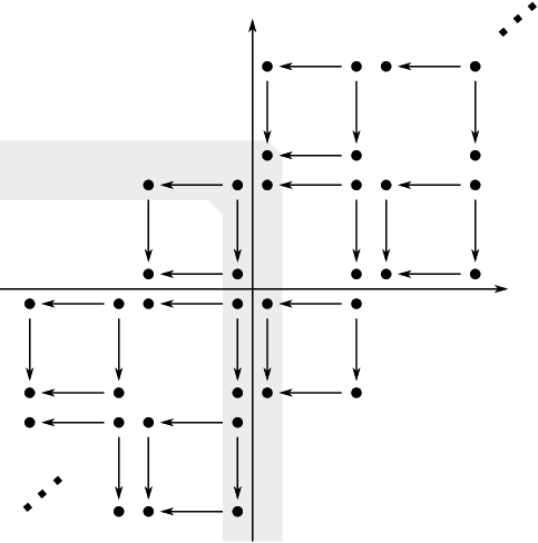
The knot Floer chain complex C​F​K∞​(S3,K)CFK^{\infty}(S^{3},K) of a homologically thin knot KK is chain homotopy equivalent to a direct sum of the model complexes called the square and the staircase of height τ⁡(K)\tau(K) depicted in Figure 2, and given as follows [Pe]. (Here, by the staircase of height hh we mean the staircase-shaped chain complex having 2​h+12h+1 generators). See Example 3.4.

Refer to caption
Figure 2. Model complex: (i) square, (ii) staircase

For i=0,1,…,i=0,1,\ldots, let εi={1i≤τ⁡(K)0i>τ⁡(K)\varepsilon_{i}=\begin{cases}1&i\leq\tau(K)\\ 0&i>\tau(K)\end{cases}, and let (δ1,…,δg)(\delta_{1},\ldots,\delta_{g}) be non-negative integers defined by the equations

|dg|\displaystyle|d_{g}| =εg+δg\displaystyle=\varepsilon_{g}+\delta_{g}
|dg−1|\displaystyle|d_{g-1}| =εg−1+δg−1+2​δg\displaystyle=\varepsilon_{g-1}+\delta_{g-1}+2\delta_{g}
|dg−2|\displaystyle|d_{g-2}| =εg−2+δg−2+2​δg−1+δg\displaystyle=\varepsilon_{g-2}+\delta_{g-2}+2\delta_{g-1}+\delta_{g}
|d2|\displaystyle|d_{2}| =ε2+δ2+2​δ3+δ4\displaystyle=\varepsilon_{2}+\delta_{2}+2\delta_{3}+\delta_{4}
|d1|\displaystyle|d_{1}| =ε1+δ1+2​δ2+δ3\displaystyle=\varepsilon_{1}+\delta_{1}+2\delta_{2}+\delta_{3}
|d0|\displaystyle|d_{0}| =ε0+2​δ1+2​δ2\displaystyle=\varepsilon_{0}+2\delta_{1}+2\delta_{2}

(When g=1g=1, the last equation is understood as d0=2​δ1+ε0d_{0}=2\delta_{1}+\varepsilon_{0}). C​F​K∞​(S3,K)CFK^{\infty}(S^{3},K) is filtered chain homotopy equivalent to the complex depicted in Figure 3.

Refer to caption
Figure 3. C​F​K∞​(S3,K)CFK^{\infty}(S^{3},K) for a homologically thin knot KK: Here we only write a complex near the filrataion (0,∗)(0,*).

Thus rank​H∗​(A^s)=2​δs+1+1\textrm{rank}\,H_{*}(\widehat{A}_{s})=2\delta_{s+1}+1 and

CK\displaystyle C_{K} =∑s∈ℤ(rank​H∗​(A^s)−1)=4​(δg+δg−1+⋯+δ2+δ1)−2​δ1\displaystyle=\sum_{s\in\mathbb{Z}}(\textrm{rank}H_{*}(\widehat{A}_{s})-1)=4(\delta_{g}+\delta_{g-1}+\cdots+\delta_{2}+\delta_{1})-2\delta_{1}

By the defining equations of δ1,…,δg\delta_{1},\ldots,\delta_{g}, we get

|dg|+|dg−1|+⋯+|d0|\displaystyle|d_{g}|+|d_{g-1}|+\cdots+|d_{0}| =(εg+⋯+ε0)+4​(δg+⋯+δ1)+(δ2−δ1)\displaystyle=(\varepsilon_{g}+\cdots+\varepsilon_{0})+4(\delta_{g}+\cdots+\delta_{1})+(\delta_{2}-\delta_{1})
=(τ+1)+4​(δg+⋯+δ1)+(δ2−δ1)\displaystyle=(\tau+1)+4(\delta_{g}+\cdots+\delta_{1})+(\delta_{2}-\delta_{1})

Hence

CK\displaystyle C_{K} =(|dg|+⋯+|d0|)−τ⁡(K)−1−(δ2−δ1)−2​δ1\displaystyle=(|d_{g}|+\cdots+|d_{0}|)-\tau(K)-1-(\delta_{2}-\delta_{1})-2\delta_{1}
=(|dg|+⋯+|d0|)−τ⁡(K)−1−(δ1+δ2)\displaystyle=(|d_{g}|+\cdots+|d_{0}|)-\tau(K)-1-(\delta_{1}+\delta_{2})
=12​(|det(K)|+|d0|)−τ⁡(K)−1−12​(|d0|−1)\displaystyle=\frac{1}{2}(|\det(K)|+|d_{0}|)-\tau(K)-1-\frac{1}{2}(|d_{0}|-1)
=12​(|det(K)|−2​|τ⁡(K)|−1)\displaystyle=\frac{1}{2}(|\det(K)|-2|\tau(K)|-1)

∎

Example 3.4.

Let KK be (the mirror image of) the knot 626_{2}, whose Alexander polynomial is t−2−3​t−1+3−3​t+t2t^{-2}-3t^{-1}+3-3t+t^{2} and τ⁡(K)=1\tau(K)=1. Thus δ2=1,δ1=0\delta_{2}=1,\delta_{1}=0, so the knot Floer chain complex C​F​K∞​(S3,K)CFK^{\infty}(S^{3},K) is given as Figure 4. The shaded region represents the complex A^1\widehat{A}_{1}.

Refer to caption
Figure 4. Example: C​F​K∞​(S3,K)CFK^{\infty}(S^{3},K) and A^1\widehat{A}_{1} for K=6¯2K=\overline{6}_{2}

4. Chirally cosmetic surgery constraint

In this section, by using the rank of the Heegaard Floer homology and constraints from the degree two finite type invariants we prove various chirally cosmetic surgery constraints in the introduction. In the following, by taking the mirror image if necessary, we assume that ν⁡(K)≥ν⁡(K¯)\nu(K)\geq\nu(\overline{K}) and ν⁡(K)≥0\nu(K)\geq 0, as in Section 3.

To begin with, let us observe that Proposition 3.1 immediately provides the following.

Proposition 4.1.

Let KK be a non-trivial knot. If SK3​(m/n)≅−SK3​(m/n′)S^{3}_{K}(m/\penalty n)\cong-S^{3}_{K}(m/\penalty n^{\prime}) (mn>mn′\frac{m}{n}>\frac{m}{n^{\prime}}), then the following holds.

  1. (i)

    mn>0\frac{m}{n}>0.

  2. (ii)

    If mn′>0\frac{m}{n^{\prime}}>0, then SK3​(m/n)S^{3}_{K}(m/\penalty n) is an L-space and CK=0C_{K}=0. In particular, mn,mn′≥2​g​(K)−1\frac{m}{n},\frac{m}{n^{\prime}}\geq 2g(K)-1.

  3. (iii)

    If 0>mn′0>\frac{m}{n^{\prime}} and ν⁡(K)=0\nu(K)=0, then n+n′=0n+n^{\prime}=0.

  4. (iv)

    If 0>mn′0>\frac{m}{n^{\prime}} and ν⁡(K)>0\nu(K)>0, then n+n′>0n+n^{\prime}>0. Moreover,

    • (iv-a)

      n+n′m=24​ν​(K)−2+CK\displaystyle\frac{n+n^{\prime}}{m}=\frac{2}{4\nu(K)-2+C_{K}} when mn≤2​ν​(K)−1\frac{m}{n}\leq 2\nu(K)-1.

    • (iv-b)

      n+n′m=(4​ν​(K)−2)​(−n′)m​CK\displaystyle\frac{n+n^{\prime}}{m}=\frac{(4\nu(K)-2)(-n^{\prime})}{mC_{K}} when mn≥2​ν​(K)−1\frac{m}{n}\geq 2\nu(K)-1 (in this case CK≠0C_{K}\neq 0).

In particular, this proves the nu-invariant constraint.

Proof of Theorem 1.5.

If KK admits a chirally cosmetic surgery of ++-type, by Proposition 4.1 (ii) CK=0C_{K}=0. Thus by (3.1) ν⁡(K)=g⁡(K)>0\nu(K)=g(K)>0. If KK admits a chirally cosmetic surgery of −--type, by Proposition 4.1 (iii) ν⁡(K)>0\nu(K)>0. ∎

We reformulate Proposition 4.1 in the following more convenient and informative form.

Corollary 4.2.

Let KK be a knot in S3S^{3}. Assume that KK admits a chirally cosmetic surgery SK3​(mn)≅−SK3​(mn′)S^{3}_{K}(\frac{m}{n})\cong-S^{3}_{K}(\frac{m}{n^{\prime}}). Then

|n+n′m|<{22​g​(K)−1(CK=0)2CK(CK>0)\left|\frac{n+n^{\prime}}{m}\right|<\begin{cases}\frac{2}{2g(K)-1}&(C_{K}=0)\\ \frac{2}{C_{K}}&(C_{K}>0)\end{cases}
Proof.

If the surgery is of 00-type, the assertion is trivial. If the surgery is of ++-type, by Corollary 4.1 (ii) mn,mn′≥2​g​(K)−1\frac{m}{n},\frac{m}{n^{\prime}}\geq 2g(K)-1. Since n≠n′n\neq n^{\prime}, n+n′m<22​g​(K)−1\frac{n+n^{\prime}}{m}<\frac{2}{2g(K)-1}.

Finally we assume that the surgery is of −--type, so mn>0>mn′\frac{m}{n}>0>\frac{m}{n^{\prime}}. By Proposition 4.1, if ν⁡(K)=0\nu(K)=0, then n+n′m=0\frac{n+n^{\prime}}{m}=0 so we have nothing to prove. Thus we assume that ν⁡(K)>0\nu(K)>0.

If mn≤2​ν​(K)−1\frac{m}{n}\leq 2\nu(K)-1, then n+n′m=24​ν​(K)−2+CK\frac{n+n^{\prime}}{m}=\frac{2}{4\nu(K)-2+C_{K}}. When CK=0C_{K}=0, g⁡(K)=ν⁡(K)g(K)=\nu(K) hence

n+n′m=12​ν​(K)−1=12​g​(K)−1<22​g​(K)−1.\frac{n+n^{\prime}}{m}=\frac{1}{2\nu(K)-1}=\frac{1}{2g(K)-1}<\frac{2}{2g(K)-1}.

When CK≠0C_{K}\neq 0, then

0<n+n′m=24​ν​(K)−2+CK<2CK.0<\frac{n+n^{\prime}}{m}=\frac{2}{4\nu(K)-2+C_{K}}<\frac{2}{C_{K}}.

If mn≥2​ν​(K)−1\frac{m}{n}\geq 2\nu(K)-1, since n+n′>0n+n^{\prime}>0, −n′n<1\frac{-n^{\prime}}{n}<1. Hence

n+n′m=(4​ν​(K)−2)​(−n′)m​CK≤2​(−n′)CK​n<2CK.\frac{n+n^{\prime}}{m}=\frac{(4\nu(K)-2)(-n^{\prime})}{mC_{K}}\leq\frac{2(-n^{\prime})}{C_{K}n}<\frac{2}{C_{K}}.

∎

Corollary 4.2 is useful; first of all, this excludes the possibility for chirally cosmetic surgery of ±\pm-type yielding integral homology spheres and homology projective space as we have mentioned in introduction.

Proof of Corollary 1.6.

Note that Corollary 4.2 implies |n+n′m|<1|\frac{n+n^{\prime}}{m}|<1 unless g⁡(K)=1g(K)=1 and CK=0C_{K}=0. However g⁡(K)=1g(K)=1 and CK=0C_{K}=0 implies that KK is the trefoil. Thanks to the classification of chirally cosmetic surgeries on the trefoil, |n+n′m|<1|\frac{n+n^{\prime}}{m}|<1 also holds in this case. When m=2m=2, n,n′n,n^{\prime} must be odd so |n+n′|=1|n+n^{\prime}|=1 never happens. ∎

Moreover as we have seen and discussed in [It1, IIS], various other invariants of 3-manifolds provide formulae of the form

SK3​(mn)≅−SK3​(mn′)\displaystyle S^{3}_{K}\left(\frac{m}{n}\right)\cong-S^{3}_{K}\left(\frac{m}{n^{\prime}}\right)
OPEN⇒n+n′m=(Some specific value(s) determined by ​K​(and ​m,n,n′))\displaystyle\Rightarrow\frac{n+n^{\prime}}{m}=\mbox{(Some specific value(s) determined by }K(\mbox{and }m,n,n^{\prime}))

(see for example, Theorem 1.3 (ii)).

Proof of Theorem 1.8.

First we assume that g⁡(K)≠ν⁡(K)g(K)\neq\nu(K). By Lemma 3.2, in this case CK≥4C_{K}\geq 4, or, g⁡(K)=1g(K)=1. Since ν⁡(K)≤g⁡(K)\nu(K)\leq g(K), when g⁡(K)=1g(K)=1, g⁡(K)≠ν⁡(K)g(K)\neq\nu(K) implies that ν⁡(K)=0\nu(K)=0. Thus by Theorem 1.5, in this case KK does not admit chirally cosmetic surgery of ±\pm-type. If CK≥4C_{K}\geq 4, by Corollary 4.2 and Theorem 1.3

|n+n′m|=|8​v3​(K)7​a2​(K)2−a2​(K)−10​a4​(K)|<2CK≤12\left|\frac{n+n^{\prime}}{m}\right|=\left|\frac{8v_{3}(K)}{7a_{2}(K)^{2}-a_{2}(K)-10a_{4}(K)}\right|<\frac{2}{C_{K}}\leq\frac{1}{2}

as desired. When g⁡(K)=ν⁡(K)g(K)=\nu(K), the assertion follows from Theorem 1.3 and Corollary 4.2 as well. ∎

Proof of Theorem 1.9.

By Lemma 3.3, Corollary 4.2, and Theorem 1.3, when SK3​(mn)≅−SK3​(mn′)S^{3}_{K}(\frac{m}{n})\cong-S^{3}_{K}(\frac{m}{n^{\prime}}),

|n+n′m|=|8​v3​(K)7​a2​(K)2−a2​(K)−10​a4​(K)|<2CK=4|det(K)|−2​|τ⁡(K)|−1.\left|\frac{n+n^{\prime}}{m}\right|=\left|\frac{8v_{3}(K)}{7a_{2}(K)^{2}-a_{2}(K)-10a_{4}(K)}\right|<\frac{2}{C_{K}}=\frac{4}{|\det(K)|-2|\tau(K)|-1}.

∎

Appendix: Formula of v5v_{5}

In this appendix we give a formula of the finite type invariant v5v_{5} in terms of the Kauffman polynomial.

Throughout the appendix, we assume some familiarity of the theory of the LMO and the Kontsevich invariant. See [Oh1], for the basics of the LMO and the Kontsevich invariant.

In [It1], we gave a formula of the degree two part λ2\lambda_{2} and the degree three part λ3\lambda_{3} of the LMO invariant, the coefficients of the Jacobi diagram and for SK3​(r)S^{3}_{K}(r). We gave a formula λ2\lambda_{2} and λ3\lambda_{3} in terms or the surgery slope rr and the finite type invariants v2,v3,v4,w4,v5,v6v_{2},v_{3},v_{4},w_{4},v_{5},v_{6} of KK, which are the coefficients of the Jacobi diagrams

            ,               ,                  ,                  ,                     ,                        \raisebox{-11.38109pt}{ \begin{picture}\put(10.0,16.0){\oval(26.0,16.0)}\put(2.0,24.0){\line{0}{1}{10.0}}\put(16.0,24.0){\line{0}{1}{10.0}}\end{picture} },\raisebox{-11.38109pt}{ \begin{picture}\put(10.0,16.0){\oval(26.0,16.0)}\put(2.0,24.0){\line{0}{1}{10.0}}\put(16.0,24.0){\line{0}{1}{10.0}}\put(-3.0,16.0){\line{1}{0}{26.0}}\end{picture} },\raisebox{-11.38109pt}{ \begin{picture}\put(10.0,16.0){\oval(26.0,16.0)}\put(2.0,24.0){\line{0}{1}{10.0}}\put(12.0,24.0){\line{0}{1}{10.0}}\put(7.0,24.0){\line{0}{1}{10.0}}\put(17.0,24.0){\line{0}{1}{10.0}}\end{picture} },\raisebox{-11.38109pt}{ \begin{picture}\put(10.0,16.0){\oval(26.0,16.0)}\put(2.0,24.0){\line{0}{1}{10.0}}\put(16.0,24.0){\line{0}{1}{10.0}}\put(-2.0,19.0){\line{1}{0}{24.0}}\put(-2.0,13.0){\line{1}{0}{24.0}}\end{picture} },\raisebox{-11.38109pt}{ \begin{picture}\put(10.0,16.0){\oval(26.0,16.0)}\put(2.0,24.0){\line{0}{1}{10.0}}\put(12.0,24.0){\line{0}{1}{10.0}}\put(7.0,24.0){\line{0}{1}{10.0}}\put(17.0,24.0){\line{0}{1}{10.0}}\put(-3.0,16.0){\line{1}{0}{26.0}}\end{picture} },\raisebox{-11.38109pt}{ \begin{picture}\put(14.0,16.0){\oval(32.0,16.0)}\put(4.0,24.0){\line{0}{1}{10.0}}\put(8.0,24.0){\line{0}{1}{10.0}}\put(12.0,24.0){\line{0}{1}{10.0}}\put(16.0,24.0){\line{0}{1}{10.0}}\put(20.0,24.0){\line{0}{1}{10.0}}\put(24.0,24.0){\line{0}{1}{10.0}}\end{picture} }

of the (wheeled) Kontsevich invariant of KK.

We also gave a formula of the finite type invariants v2,v3,v4,w4,v6v_{2},v_{3},v_{4},w_{4},v_{6} in terms of the Conway and the Jones polynomial. However, we did not give an explicit formula of v5v_{5}, because v5v_{5} is not determined by the Conway polynomial and the Jones polynomial, and, in the applications discussed in [It1] we do not need computations of the actual value of v5v_{5}.

In [It1] we used the 𝔰​𝔩2\mathfrak{sl}_{2} weight system evaluation to get a formula of v3,w4v_{3},w_{4}. A similar argument using 𝔰​𝔬n\mathfrak{so}_{n} weight system works for v5v_{5}, but here we give a slightly different approach.

A finite type invariant vv of degree nn is canonical if there is a weight system w:ℬ→ℂw:\mathcal{B}\rightarrow\mathbb{C} of degree nn (i.e. w⁡(D)=0w(D)=0 whenever the degree of DD is not equal to nn) such that v⁡(K)=w⁡(Zσ​(K))v(K)=w(Z^{\sigma}(K)). Here ℬ\mathcal{B} denotes the space of the open Jacobi diagrams and Zσ​(K)∈ℬZ^{\sigma}(K)\in\mathcal{B} denotes the Kontsevich invariant (taken so that it takes value in ℬ\mathcal{B} by composing the inverse of the PBW isomorphism σ\sigma). In other words, vv is canonical if it is written as a linear combination of the coefficients of the degree nn part of the Kontsevich invariant. Thus by definition, v5v_{5} is a canonical finite type invariant of degree 55.

On the other hand, we can extract canonical finite type invariants from the Kauffman polynomial as follows.

Lemma A.3.

Let FK​(a,z)F_{K}(a,z) be the Kauffman polynomial of a knot KK and N≥1N\geq 1 be a positive integer. We expand FK​(a,z)F_{K}(a,z) as a formal power series of hh

(A.1) FK​(i​eN​h,−i⁡(eh−e−h))=∑h≥0kn,N​(K)​hnF_{K}(ie^{Nh},-i(e^{h}-e^{-h}))=\sum_{h\geq 0}k_{n,N}(K)h^{n}

where i=−1i=\sqrt{-1}. Then kn,N​(K)k_{n,N}(K) is a canonical finite type invariant of degree nn.

Proof.

Let DK​(a,z)D_{K}(a,z) be the Dubrovnik polynomial, a version of the Kauffman polynomial given by

DK​(a,z)=(−1)#​K−1​FK​(i​a,−i​z).D_{K}(a,z)=(-1)^{\#K-1}F_{K}(ia,-iz).

Here #​K\#K denotes the number of component of KK. It is known that DK​(eN​h,eh−e−h)D_{K}(e^{Nh},e^{h}-e^{-h}) is equal to the quantum (𝔰​𝔬4​N+1,V)(\mathfrak{so}_{4N+1},V)-invariant Q𝔰​𝔬4​N+1;V​(K)Q^{\mathfrak{so}_{4N+1};V}(K) [MPS], where VV is the standard representation of 𝔰​𝔬4​N+1\mathfrak{so}_{4N+1}. Thus for each NN, the expansion (A.1) is nothing but an expansion of the quantum (𝔰​𝔬4​N+1,V)(\mathfrak{so}_{4N+1},V)-invariant

Q𝔰​𝔬4​N+1;V​(K)\displaystyle Q^{\mathfrak{so}_{4N+1};V}(K) =∑h≥0kn,N​(K)​hn.\displaystyle=\sum_{h\geq 0}k_{n,N}(K)h^{n}.

By [Ka, Theorem XX.8.3], kn,Nk_{n,N} is a canonical finite type invariant of degree nn. ∎

It is known that the dimension of the degree 55 part of ℬ\mathcal{B} is four. By computing k5,2,k5,3,k5,4,k5,5k_{5,2},k_{5,3},k_{5,4},k_{5,5} for several knots, one can confirm they are linearly independent so they form a basis of canonical finite type invariants of degree 55. Therefore we may write

v5=x1​k5,2+x2​k5,3+x3​k5,4+x4​k5,5v_{5}=x_{1}k_{5,2}+x_{2}k_{5,3}+x_{3}k_{5,4}+x_{4}k_{5,5}

where x1,x2,x3,x4∈ℝx_{1},x_{2},x_{3},x_{4}\in\mathbb{R} are constants.

The coefficients x1,x2,x3,x4x_{1},x_{2},x_{3},x_{4} are determined by computing v5,k5,2,k5,3,k5,4,k5,5v_{5},k_{5,2},k_{5,3},k_{5,4},k_{5,5} for suitable knots. Since we can compute the Kauffman polynomial, the computation of k5,2,k5,3,k5,4,k5,5k_{5,2},k_{5,3},k_{5,4},k_{5,5} are routine.

To compute v5v_{5} for some specific knots, we use the reduced 2-loop polynomial Θ^K​(t)\widehat{\Theta}_{K}(t) of KK. The reduced 2-loop polynomial is an invariant of a knot that comes from the 𝔰​𝔩2\mathfrak{sl}_{2} weight system evaluation of the two-loop part of the Kontsevich invariant. For details of the 2-loop polynomial we refer to [Oh2, Oh3].

We express v5v_{5} in terms of the reduced 2-loop polynomial Θ^K​(t)\widehat{\Theta}_{K}(t).

Lemma A.4.

Let LK​(x)=Θ^K​(ex)ΔK​(ex)2L_{K}(x)=\frac{\widehat{\Theta}_{K}(e^{x})}{\Delta_{K}(e^{x})^{2}}, where ΔK​(t)\Delta_{K}(t) is the Alexander polynomial, normalized so that ΔK​(t)=ΔK​(t−1)\Delta_{K}(t)=\Delta_{K}(t^{-1}), ΔK​(1)=1\Delta_{K}(1)=1. Then

v5​(K)=116​(16​LK​(0)+LK′′​(0))v_{5}(K)=\frac{1}{16}\left(\frac{1}{6}L_{K}(0)+L_{K}^{\prime\prime}(0)\right)

In particular, when ΔK​(t)=1\Delta_{K}(t)=1 then

v5​(K)=116​(16​Θ^K​(1)+Θ^K′′​(1))v_{5}(K)=\frac{1}{16}\left(\frac{1}{6}\widehat{\Theta}_{K}(1)+\widehat{\Theta}_{K}^{\prime\prime}(1)\right)
Proof.

This follows from the same argument as [Oh2, Proposition 5.1], where it was proven that v3​(K)=18​Θ^​(1)v_{3}(K)=\frac{1}{8}\widehat{\Theta}(1).

Let WW be the map that sends a labelled 2-loop Jacobi diagram to ℚ⁡[[x]]\mathbb{Q}[[x]], given by

W(         f1​(x)   f2​(x)   f3​(x)   )=16∑{i,j,k}={1,2,3}fi(x)fj(−x)fk(0)W\left(\raisebox{-22.76219pt}{ \begin{picture}\put(30.0,25.0){\oval(60.0,35.0)}\put(0.0,25.0){\line{1}{0}{60.0}}\put(20.0,48.0){\footnotesize$f_{1}(x)$}\put(20.0,29.0){\footnotesize$f_{2}(x)$}\put(20.0,10.0){\footnotesize$f_{3}(x)$}\end{picture} }\right)=\frac{1}{6}\sum_{\{i,j,k\}=\{1,2,3\}}f_{i}(x)f_{j}(-x)f_{k}(0)

Here fi​(x)∈ℚ​[[x]]f_{i}(x)\in\mathbb{Q}[[x]] is a formal power series of xx, and a Jacobi diagram whose edge is labeled by a power series f⁡(x)=c0+c1​x+c2​x2+c3​x3+⋯f(x)=c_{0}+c_{1}x+c_{2}x^{2}+c_{3}x^{3}+\cdots represents the Jacobi diagram

      f⁡(x)   =c0      +c1         +c2            +c3               +⋯.\raisebox{-11.38109pt}{ \begin{picture}\put(2.0,0.0){\line{0}{1}{30.0}}\put(5.0,22.0){\scriptsize$f(x)$}\end{picture} }=c_{0}\raisebox{-11.38109pt}{ \begin{picture}\put(2.0,0.0){\line{0}{1}{30.0}}\end{picture} }+c_{1}\raisebox{-11.38109pt}{ \begin{picture}\put(2.0,0.0){\line{0}{1}{30.0}}\put(2.0,15.0){\line{1}{0}{10.0}}\end{picture} }+c_{2}\raisebox{-11.38109pt}{ \begin{picture}\put(2.0,0.0){\line{0}{1}{30.0}}\put(2.0,12.0){\line{1}{0}{10.0}}\put(2.0,18.0){\line{1}{0}{10.0}}\end{picture} }+c_{3}\raisebox{-11.38109pt}{ \begin{picture}\put(2.0,0.0){\line{0}{1}{30.0}}\put(2.0,9.0){\line{1}{0}{10.0}}\put(2.0,15.0){\line{1}{0}{10.0}}\put(2.0,21.0){\line{1}{0}{10.0}}\end{picture} }+\cdots.

The map WW sends the 2-loop part of the logarithm of the Kontsevich invariant to

112​(ex2−e−x2)2​LK​(x)\frac{1}{12}(e^{\frac{x}{2}}-e^{-\frac{x}{2}})^{2}L_{K}(x)

which is viewed as a formal power series by taking the Taylor expansion at x=0x=0;

112​(ex2−e−x2)2​LK​(x)=c0+c1​x+c2​x2+c3​x3+x4​x4+⋯.\frac{1}{12}(e^{\frac{x}{2}}-e^{-\frac{x}{2}})^{2}L_{K}(x)=c_{0}+c_{1}x+c_{2}x^{2}+c_{3}x^{3}+x_{4}x^{4}+\cdots.

Since v5v_{5} is the defined as the coefficient of the 2-loop Jacobi diagram and

W(                     )=W(         x4   1   1   )=23x4,W\left(\raisebox{-11.38109pt}{ \begin{picture}\put(10.0,16.0){\oval(26.0,16.0)}\put(2.0,24.0){\line{0}{1}{10.0}}\put(12.0,24.0){\line{0}{1}{10.0}}\put(7.0,24.0){\line{0}{1}{10.0}}\put(17.0,24.0){\line{0}{1}{10.0}}\put(-3.0,16.0){\line{1}{0}{26.0}}\end{picture} }\right)=W\left(\raisebox{-22.76219pt}{ \begin{picture}\put(25.0,25.0){\oval(50.0,35.0)}\put(0.0,25.0){\line{1}{0}{50.0}}\put(20.0,46.0){\footnotesize$x^{4}$}\put(20.0,29.0){\footnotesize$1$}\put(20.0,10.0){\footnotesize$1$}\end{picture} }\right)=\frac{2}{3}x^{4},

we conclude that

v5\displaystyle v_{5} =32​c4=32​(14!​d4d​x4​(112​(ex2−e−x2)2​LK​(x))|x=0)\displaystyle=\frac{3}{2}c_{4}=\frac{3}{2}\left(\frac{1}{4!}\frac{d^{4}}{dx^{4}}\left.\left(\frac{1}{12}(e^{\frac{x}{2}}-e^{-\frac{x}{2}})^{2}L_{K}(x)\right)\right|_{x=0}\right)
=116​(16​LK​(0)+LK′′​(0))\displaystyle=\frac{1}{16}\left(\frac{1}{6}L_{K}(0)+L_{K}^{\prime\prime}(0)\right)

∎

The reduced 2-loop polynomial is computed for the torus knot T⁡(p,q)T(p,q) [Oh2, Corollary 3.1] and the genus one knots [Oh2, Corollary 3.1]. Using these results and Lemma A.4, we compute values of v5,k5,2,k5,3,k5,4,k5,5v_{5},k_{5,2},k_{5,3},k_{5,4},k_{5,5} for several knots. The results are presented in Table 3. Here J⁡(ℓ,m)J(\ell,m) denotes the double twist knot.

Knot v5v_{5} k5,2k_{5,2} k5,3k_{5,3} k5,4k_{5,4} k5,5k_{5,5}
T⁡(2,3)T(2,3) −17/48-17/48 −176-176 −736-736 −1056-1056 12801280
T⁡(2,5)T(2,5) −229/48-229/48 −2480-2480 −11360-11360 −21024-21024 −3840-3840
J⁡(−2,4)J(-2,4) 37/1637/16 11041104 41284128 35523552 −19200-19200
J⁡(2,4)J(2,4) 43/4843/48 464464 27202720 96969696 2688026880
Table 3. Values of the finite type invariants v5,v5,2,v5,3,v5,4v_{5},v_{5,2},v_{5,3},v_{5,4} and v5,5v_{5,5} for some specific knots

From this computation, we get an explicit formula of v5v_{5} in terms of the Kauffman polynomial.

Theorem A.5.
v5​(K)=1768​k5,2​(K)+1768​k5,3​(K)−11536​k5,4​(K)+761440​k5,5​(K)v_{5}(K)=\dfrac{1}{768}k_{5,2}(K)+\dfrac{1}{768}k_{5,3}(K)-\dfrac{1}{1536}k_{5,4}(K)+\dfrac{7}{61440}k_{5,5}(K)

References

  • [BHW] S. Bleiler, C. Hodgson and J. Weeks, Cosmetic surgery on knots, in Proceedings of the Kirbyfest (Berkeley, CA, 1998), 23–34, Geom. Topol. Monogr., 2, Geom. Topol. Publ., Coventry.
  • [De] R. Detcherry, A quantum obstruction to purely cosmetic surgeries arXiv:2102.11323v1.
  • [FKP] D. Futer, E. Kalfagianni, and J. Purcell, Dehn filling, volume, and the Jones polynomial. J. Differential Geom. 78 (2008), no. 3, 429–464.
  • [FPS] D. Futer, J. Purcell and S. Schleimer, Effective bilipschitz bounds on drilling and filling, Geom. Topol., to appear.
  • [GL] C. Gordon and J. Luecke, Knots are determined by their complements, J. Amer. Math. Soc. 2 (1989), 371–415.
  • [Ha] J. Hanselman, Heegaard Floer homology and cosmetic surgeries in S3S^{3}. J. Eur. Math. Soc. to appear.
  • [HRW] M. Hedden, J. Rasmussen and L. Watson, Heegaard Floer homology for manifolds with torus boundary: properties and examples, arXiv:1810.10355v1.
  • [HW] M. Hedden and L. Watson, On the geography and botany of knot Floer homology, Selecta Math. (N.S.) 24 (2018), no. 2, 997–1037.
  • [HIKMOT] N. Hoffman, K. Ichihara, M. Kashiwagi, M. Hidetoshi and S. Oishi, A. Takayasu, Verified computations for hyperbolic 3-manifolds. Exp. Math. 25 (2016), no. 1, 66–78.
  • [IIS] K. Ichihara, T. Ito and T. Saito, Chirally cosmetic surgeries and Casson invariants. Tokyo J. Math, 44 (2021), no. 1, 1–24.
  • [IJMS] K. Ichihara, I. D. Jong, T, Mattman and T. Saito, Two-bridge knots admit no purely cosmetic surgeries. Algebr. Goem. Topol, 21 (2021), no. 5, 2411–2424.
  • [IJ] K. Ichihara and I. D. Jong, Cosmetic banding on knots and links, Osaka J. Math. 55 (2018), no. 4, 731–745.
  • [IW] K. Ichihara, and Z. Wu, A note on Jones polynomial and cosmetic surgery, Comm. Anal. Geom. 27 (2019), no. 5, 1087–1104.
  • [It1] T. Ito, On LMO invariant constraints for cosmetic surgery and other surgery problems for knots in S3S^{3}, Comm. Anal. Geom. 28 (2020), no. 2, 321–349.
  • [It2] T. Ito, A note on chirally cosmetic surgery on cable knots, Canad. Math. Bull. 64 (2021), no. 1, 163–173.
  • [It3] T. Ito, A remark on a finiteness of purely cosmetic surgeries, arXiv:2104.07922v1.
  • [Ka] C. Kassel, Quantum groups, Graduate Texts in Mathematics, 155. Springer-Verlag, New York, 1995. xii+531 pp.
  • [Ke] M. Kegel, private communication.
  • [KM] R. Kirby and P. Melvin, The 3-manifold invariants of Witten and Reshetikhin-Turaev for 𝔰​𝔩​(2,ℂ)\mathfrak{sl}(2,\mathbb{C}), Invent. Math. 105 (1991), no. 3, 473–545.
  • [LM] C. Livingston and A. Moore, KnotInfo: Table of Knot Invariants, knotinfo.math.indiana.edu, December 1, 2021.
  • [NW] Y. Ni and Z. Wu, Cosmetic surgeries on knots in S3S^{3}, J. Reine Angew. Math. 706 (2015), 1–17.
  • [MO] C. Manolescu and P. Ozsváth, On the Khovanov and knot Floer homologies of quasi-alternating links, Proceedings of Gökova Geometry-Topology Conference 2007, 60–81, Gökova Geometry/Topology Conference (GGT), Gökova, 2008.
  • [MPS] S. Morrison, E. Peters, and N. Snyder, Knot polynomial identities and quantum group coincidences, Quantum Topol. 2 (2011), no. 2, 101–156.
  • [Oh1] T. Ohtsuki, Quantum Invariants, Series on Knots and Everything 29, World Scientific Publishing Co., Inc., River Edge, NJ, (2002)
  • [Oh2] T. Ohtsuki, A cabling formula for the 2-loop polynomial of knots, Publ. Res. Inst. Math. Sci. 40 (2004), no. 3, 949–971.
  • [Oh3] T. Ohtsuki, On the 2-loop polynomial of knots, Geom. Topol. 11 (2007), 1357–1475.
  • [OS1] P. S. Ozsváth and Z. Szabó, Heegaard Floer homology and alternating knots, Geom. Topol. 7 (2003), 225–254.
  • [OS2] P. S. Ozsváth and Z. Szabó, Knot Floer homology and rational surgeries, Algebr. Geom. Topol. 11 (2011), no. 1, 1–68.
  • [Pe] I. Petkova, Cables of thin knots and bordered Heegaard Floer homology, Quantum Topol. 4 (2013), 377–409.
  • [SZ] A. Stipsicz and Z. Szabó, Purely cosmetic surgeries and pretzel knots arXiv:2006.06765v1
  • [Ta1] R. Tao, Cable knots do not admit cosmetic surgeries, J. Knot Theory Ramifications 28 (2019), no. 4, 1950034, 11 pp.
  • [Ta2] R. Tao, Connected sums of knots do not admit purely cosmetic surgeries, arXiv:1909.05048v1.
  • [Va1] K. Varvarezos, Alternating odd pretzel knots and chirally cosmetic surgeries, arXiv:2003.08442v1.
  • [Va2] K. Varvarezos, Heegaard Floer homology and chirally cosmetic surgeries, arXiv:2112.03144v1.