Model-Value Inconsistency as a Signal for Epistemic Uncertainty

Angelos Filos Affiliation: DeepMind Affiliation: University of Oxford Correspondence to: angelos.filos@cs.ox.ac.uk Eszter Vértes Affiliation: DeepMind Zita Marinho Affiliation: DeepMind Gregory Farquhar Affiliation: DeepMind Diana Borsa Affiliation: DeepMind Abram Friesen Affiliation: DeepMind Feryal Behbahani Affiliation: DeepMind Tom Schaul Affiliation: DeepMind André Barreto Affiliation: DeepMind Simon Osindero Affiliation: DeepMind

Abstract

Using a model of the environment and a value function, an agent can construct many estimates of a state’s value, by unrolling the model for different lengths and bootstrapping with its value function. Our key insight is that one can treat this set of value estimates as a type of ensemble, which we call an implicit value ensemble (IVE). Consequently, the discrepancy between these estimates can be used as a proxy for the agent’s epistemic uncertainty; we term this signal model-value inconsistency or self-inconsistency for short. Unlike prior work which estimates uncertainty by training an ensemble of many models and/or value functions, this approach requires only the single model and value function which are already being learned in most model-based reinforcement learning algorithms. We provide empirical evidence in both tabular and function approximation settings from pixels that self-inconsistency is useful (i) as a signal for exploration, (ii) for acting safely under distribution shifts, and (iii) for robustifying value-based planning with a learned model.

Keywords:

Machine Learning, Reinforcement Learning, Planning, Epistemic Uncertainty,

^†^†affiliationnotice: Equal contribution

1 Introduction

Refer to caption — a Implicit Value Ensemble (IVE)

a Value Ensemble (EVE)

b Model Ensemble (EMVE)

c Implicit Value Ensemble (IVE)

Figure 2: Value computation in scalable epistemic uncertainty-aware RL agents. (a-b) Explicit ensemble of value functions (Osband et al. 2016) and world models (Chua et al. 2018), approximating samples from

p(v|\mathcal{B})

and

p(m|\mathcal{B})

, respectively. The number of parameters grows linearly with the ensemble size. (c) Implicit value ensemble (IVE) make ensemble value predictions using a single learned value function and world model by exploiting the model-induced Bellman operator

\mathcal{T}_{\hat{m}}

and the Bellman consistency of the “true” model

m^{*}

and value function

v

, keeping the number of parameters constant.

Agents that employ learning to improve their decision making should be equipped with mechanisms for representing and using their acquired knowledge effectively. Learned models of the environment (Sutton 1991) and value functions (Sutton 1988) are explicit ways that reinforcement learning (Sutton & Barto 2018, RL,) agents use to represent their knowledge about the environment.

Equally important is the agents’ ability to reason about their ignorance (Strens 2000, i.e., epistemic uncertainty,) and factor it in their decisions (Milnor 1951). In tabular settings, exact Bayesian inference can be used for quantifying the agents’ uncertainty in both model-free (Dearden et al. 1998) and model-based (Dearden et al. 1999) RL approaches. However, in complex RL problems, since exact Bayesian inference is intractable, proxy signals are often used instead, including prediction error (Lopes et al. 2012; Pathak et al. 2017), approximate state visitation counts (Bellemare et al. 2016) and disagreement of samples from either approximate posterior distributions over learned parameters (Blundell et al. 2015) or explicit ensembles of value functions (Osband et al. 2016) or world models (Chua et al. 2018).

In this work, we introduce a novel signal for capturing RL agents’ ignorance, termed model-value inconsistency or self-inconsistency for short. A $k$ -step self-inconsistency signal is constructed by applying the model-induced Bellman operator $\mathcal{T}_{\hat{m}}$ to learned value function $\hat{v}$ , $k$ times. This produces $k+1$ different estimates of the state value: $\{\hat{v},\mathcal{T}_{\hat{m}}\hat{v},(\mathcal{T}_{\hat{m}})^{2}\hat{v},\ldots,(\mathcal{T}_{\hat{m}})^{k}\hat{v}\}$ , as illustrated in Figures 1 and 2c. Our key insight is that these can be thought of as predictions from an ensemble of value functions, which we call the implicit value ensemble (IVE).

Consequently, the disagreement of these predictions can tell us about the agent’s uncertainty in the value of a state. The intuition behind this is based on the fact that the true model and value are by definition Bellman-consistent. As a result, for regions of the state space where the learned model and value are accurate, we expect the self-inconsistency to be low. Conversely, high self-inconsistency can signal that the learned model-value pair is inaccurate.

In contrast to prior work that requires explicit ensembles of learned value functions (Osband et al. 2016; Lowrey et al. 2018) or ensembles of world models (Chua et al. 2018; Sekar et al. 2020), self-inconsistency can be efficiently calculated by any RL agent that has a learned (approximate) model of the environment and value function, see Figure 2. Moreover, unlike model-ensembles, self-inconsistency captures the agents’ ignorance about behaviourally-relevant quantities, i.e., rewards and values, and hence is robust to irrelevant information for control noise (Schmidhuber 2010).

We provide empirical evidence that self-inconsistency provides a proxy of epistemic uncertainty (Section 4.1), and that this information can be used to guide exploration or act safely (Section 4.2), and to robustify planning (Section 4.3).

2 Background

We model the agent’s interaction with the environment as a Markov decision process (Puterman 2014, MDP,), i.e., $\mathcal{M}\triangleq\left(\mathcal{S},\mathcal{A},p,r\right)$ . At any discrete time step $t\geq 0$ , the agent is in state $s_{t}\in\mathcal{S}$ , takes an action $a_{t}\in\mathcal{A}$ , according to a policy $\pi:\mathcal{S}\rightarrow\Delta(\mathcal{A})$ , then receives reward $R_{t+1}\sim r(\cdot|s_{t},a_{t})\in\mathbb{R}$ and transitions to the state $S_{t+1}\sim p(\cdot|s_{t},a_{t})$ . For brevity, the “true” model is denoted by $m^{*}\triangleq(p,r)$ and we write $S_{t+1},R_{t+1}\sim m^{*}(\cdot,\cdot|s_{t},a_{t})$ . The agent’s goal is to find the policy that maximises the value of each state, for a discount factor $\gamma\in[0,1)$ , $v^{\pi}(s)\triangleq\mathbb{E}_{\pi,m^{*}}[\sum_{t\geq 0}\gamma^{t}R_{t}|S_{0}=s]$ , where $\mathbb{E}_{\pi,m^{*}}\left[\cdot\right]$ denotes the expectation¹¹ 1 In this work, we only construct estimates of the mean of the returns distribution (Bellemare et al. 2017, a.k.a value distribution) and hence environment and policy stochasticity is integrated out. over the trajectories induced by running policy $\pi$ in the environment $m^{*}$ , starting from state $s$ .

The computation of the value of a policy $\pi$ , i.e., $v^{\pi}$ , is termed policy evaluation and can be concisely formulated using Bellman evaluation operators (Bellman 1957). Next, we define the one-step Bellman evaluation operator, applied on a state-(to-scalar) function $v\in\mathbb{V}\triangleq\{f:\mathcal{S}\rightarrow\mathbb{R}\}$ .

Definition 1 (Bellman evaluation operator).

Given the model $m^{*}$ and policy $\pi$ the one-step Bellman evaluation operator $\mathcal{T}^{\pi}:\mathbb{V}\rightarrow\mathbb{V}$ is induced, and its application on a state-function $v\in\mathbb{V}$ , for all $s\in\mathcal{S}$ , is given by

\displaystyle\mathcal{T}^{\pi}v(s)\triangleq\mathbb{E}_{\pi,m^{*}}\left[R_{1}+\gamma v(S_{1})\mid S_{0}=s\right].

(1)

The $k$ -times repeated application of an one-step Bellman operator gives rise to the $k$ -steps Bellman operator,

\displaystyle(\mathcal{T}^{\pi})^{k}v\triangleq\hskip 1.19995pt\underbracket{\mathcal{T}^{\pi}\cdots\mathcal{T}^{\pi}\hskip 0.0pt}_{k\text{-times}}v.

(2)

The Bellman evaluation operator, $\mathcal{T}^{\pi}$ , is a contraction mapping (Puterman 2014), and its fixed point is the value of the policy $\pi$ , i.e., $\lim_{n\rightarrow\infty}(\mathcal{T}^{\pi})^{n}v=v^{\pi}$ , for any $v\in\mathbb{V}$ .

2.1 Model-Based Reinforcement Learning

In the general RL formulation, it is assumed that the environment model $m^{*}$ is unknown to the agent (Sutton & Barto 2018) which thus cannot directly compute Eqn. (1). Model-free RL agents resolve this by estimating these expectations through sampling. Model-based RL agents, the focus of this paper, learn an approximate model $\hat{m}\approx m^{*}$ , possibly together with a learned value function $\hat{v}\approx v^{\pi}$ (Sutton 1991), and use them to compute an estimate of the value, by replacing model and function $m^{*}$ , $v$ with $\hat{m}$ , $\hat{v}$ in Eqn. (1).

Model-induced Bellman operator.

A model $\hat{m}$ and policy $\pi$ induce a Bellman evaluation operator $\mathcal{T}_{\hat{m}}^{\pi}$ with a fixed point $v_{\hat{m}}^{\pi}$ . Similar to Eqn. (2), a $k$ -steps model-induced Bellman operator is given by $(\mathcal{T}_{\hat{m}}^{\pi})^{k}v=\hskip 1.19995pt\underbracket{\mathcal{T}_{\hat{m}}^{\pi}\cdots\mathcal{T}_{\hat{m}}^{\pi}\hskip 0.0pt}_{k\text{-times}}v$ .

Model learning principles.

The agent interacts with the environment, generating a sequence of states, actions and rewards, which we denote with $\mathcal{B}\triangleq\{(s_{t},a_{t},r_{t})\}_{t\geq 0}$ .

Maximum likelihood estimation (Kumar & Varaiya 2015; Sutton 1991, MLE,) can be used for learning the model parameters, given experience tuples $(s,a,r^{\prime},s^{\prime})\sim\mathcal{B}$ ,

\displaystyle\hat{m}_{\text{MLE}}=\argmax_{m}\mathbb{E}_{\mathcal{B}}\left[\log m(r^{\prime},s^{\prime}\mid s,a)\right].

(3)

Action-conditioned hidden Markov models have been used to scale MLE methods to high-dimensional environments (Watter et al. 2015), e.g., with pixel observations.

Value equivalence (Grimm et al. 2021, VE,) is an alternative principle for model learning. It selects the model that induces the “best” approximation to the $k$ -th order Bellman operator of the environment, applied on state-functions $\mathcal{V}$ , policies $\Pi$ and state $s$ , trained via samples $(s,a,r^{\prime},s^{\prime})\sim\mathcal{B}$ ,

\displaystyle\hat{m}_{\text{VE}}=\argmin_{m}\mathbb{E}_{\mathcal{B}}\!\!\!\!\!\sum_{\pi\in\Pi,v\in\mathcal{V}}\!\!\!\!\!\left|(\mathcal{T}_{m}^{\pi})^{k}v(s)-(\mathcal{T}^{\pi})^{k}v(s)\right|.

(4)

2.2 Epistemic-Uncertainty-Aware Agents

We refer to learning agents that can quantify their uncertainty about their learned components, e.g., value function or model, as epistemic uncertainty-aware (a.k.a. ignorance-aware) agents. While aleatoric uncertainty captures the inherent and irreducible stochasticity of the agents’ environment, epistemic uncertainty is agent-centric (Savage 1972, i.e., subjective,) and reducible (Hutter 2004).

Bayesian agents.

A principled approach to quantifying epistemic uncertainty is by treating learned quantities as random variables and perform Bayesian inference given the observed data. Bayesian RL agents maintain beliefs over value functions (Dearden et al. 1998) or world models (Dearden et al. 1999), which are updated upon interactions with the environment. Exact inference is intractable for most interesting problems and thus ensemble-based approximations are used instead (Lu et al. 2021).

Explicit ensemble methods.

In deep RL, neural networks (NNs) are used to approximate the value function (Mnih et al. 2013) or the model (Watter et al. 2015). A popular approach to epistemic uncertainty quantification for NNs is deep ensembles (Lakshminarayanan et al. 2016). Under certain assumptions (Pearce et al. 2020), the ensemble components can be seen as samples from the posterior distribution over NN parameters. It has been argued that the diversity (i.e., de-correlation) of the ensemble components is important for better capturing epistemic uncertainty (Wilson & Izmailov 2020) and various methods have been used to achieve this, all of which inject noise into the learning algorithm, such as: (i) data bootstrapping (Tibshirani 1996; Osband et al. 2016); (ii) different loss function (iii) function form (Wenzel et al. 2020) or (iv) structured noise per ensemble component (Osband et al. 2018, e.g., priors,).

RL agents with an ensemble of value functions or models have been used to quantify their epistemic uncertainty e.g. (Osband et al. 2016; Kurutach et al. 2018), see Figure 2a and 2b, respectively. We call these methods explicit ensemble methods and their number of parameters grows linearly with the ensemble size. In contrast, implicit ensembles escape this linear scaling by sharing parameters between the ensemble members but without sacrificing diversity.

3 Your Model-Based Agent is Secretly an Ensemble of Value Functions

We now present a proxy signal for epistemic uncertainty, computable by any model-based RL agent with a single (point) estimate of a world model and a value function²² 2 In this section, we define everything in terms of the Bellman evaluation operator and an approximate on-policy value function. The Bellman optimality operator and an approximate optimal value function could be used instead. For completeness, see Appendix C..

3.1 Implicit Value Ensemble

A key component of our method is the value estimated by a $k$ -step application of the model-induced Bellman operator on the learned value function, which we call $k$ -steps model-predicted value³³ 3 Similar quantities have been used in prior work, e.g., $k$ -preturn (Silver et al. 2017) and MVE (Feinberg et al. 2018). We discuss them and their differences in more detail in Section 5. ( $k$ -MPV), given by

\displaystyle\hat{v}_{\hat{m}}^{k}\triangleq(\mathcal{T}_{\hat{m}}^{\pi})^{k}\hat{v}.

(5)

The

k

-MPV is a value estimator that interpolates between (i) a model-free value estimator, i.e.,

k=0

and (ii) a purely model-based value estimator, i.e.,

k\rightarrow\infty

$k$ -MPV and $n$ -step returns.

The $k$ -MPV should not be confused with the $n$ -step returns used in temporal difference (Sutton 1988, TD,) learning. The former is an agent’s estimate about its value, i.e., $\hat{v}_{\hat{m}}^{k}\approx v^{\pi}$ that uses both the learned value function and model. The latter is a stochastic estimate of the environment’s $n$ -step Bellman operator that can be used for constructing value target estimators in TD learning with reduced bias.

An ensemble of $k$ -MPV predictions can be made by varying $k$ . We call this an implicit value ensemble⁴⁴ 4 Non-successive values of $k$ can be used in the construction of an IVE, e.g., $k\in\{1,7,13\}$ , but in practice this is less computationally efficient, see Section 3.3. (IVE), depicted in Figure 1a and 2c and denoted by

\displaystyle\{\hat{v}_{\hat{m}}^{i}\}_{i=0}^{n}\triangleq\hskip 1.19995pt\underbracket{\{\hat{v},\mathcal{T}_{\hat{m}}^{\pi}\hat{v},\ldots,(\mathcal{T}_{\hat{m}}^{\pi})^{n}\hat{v}\}\hskip 0.0pt}_{n+1\text{ value estimates}}.

(6)

Any agent with a model and value function is, in effect, also equipped with an ensemble of value functions.

3.2 Model-Value Inconsistency

We term the disagreement of the IVE components as model-value inconsistency or just self-inconsistency, for short, since it quantifies the Bellman-inconsistency (Farquhar et al. 2021) of the learned model and value function.

As our learned model and value function better approximate their “true” counterparts, the self-inconsistency reduces since the “true” model and value function are Bellman consistent, i.e., $(\mathcal{T}_{m^{*}}^{\pi})^{n}v^{\pi}=(\mathcal{T}_{m^{*}}^{\pi})^{l}v^{\pi},\forall n,l\in\mathbb{N}$ . If the true model and value function are contained in the hypothesis classes of our approximators and the respective learning algorithms converge to the “true” solutions, then the self-inconsistency reduces to zero.

In regions of state space where the learned model and value function are accurate, they are also self-consistent. With high self-inconsistency the learned model or/and value should be inaccurate.

Various metrics can be used to quantify the disagreement between the IVE components. Since the $k$ -MPVs are scalars, we can use any measure of disagreement of its components, e.g., the standard deviation across the IVE members, denoted by $\sigma$ -IVE( $n$ ) for $n$ members. Similarly, we define $\mu$ -IVE( $n$ ) as the value prediction, given by the ensemble mean, and $\mu+\beta\cdot\sigma$ -IVE( $n$ ) as the weighted sum of the IVE mean and standard deviation, where $\beta\in\mathbb{R}$ . We can induce a self-inconsistency- (i) seeking; (ii) averse or (iii) neutral policy when $\beta>0$ , $\beta<0$ and $\beta=0$ , respectively.

3.3 Practical Implementation

We use parametric function approximators, in particular neural networks, to approximate the model and value function: $\theta$ are the model and $\phi$ are the value function parameters, from hypotheses classes $\Theta$ and $\Phi$ , respectively, i.e., $\hat{m}(\cdot,\cdot|s,a;\theta)\approx m^{*}(\cdot,\cdot|s,a)$ and $\hat{v}(s;\phi)\approx\hat{v}(s)$ .

With small tabular models, such as the ones used for the gridworld in Figure 3, we can calculate the $k$ -MPVs exactly. With neural network models, the calculation of the expectation in Eqn. (1) is generally intractable and hence we can only approximate it, e.g., in the case of stochastic models, via Monte Carlo (MC) sampling. An MC sample of the $k$ -MPV of state $s\in\mathcal{S}$ is given by:

\displaystyle\mathbf{\hat{v}_{\hat{m}}^{k}}(s)=\sum_{i=1}^{k-1}\gamma^{i-1}\mathbf{r_{\hat{m}}^{i+1}}+\gamma^{k}\hat{v}(\mathbf{s_{\hat{m}}^{k}}),

(7)

where $\mathbf{s_{\hat{m}}^{0}}=s$ and the samples from the model and policy are in bold and subscripted with $\hat{m}$ and $\pi$ , i.e., $\mathbf{r_{\hat{m}}^{i+1}},\mathbf{s_{\hat{m}}^{i+1}}\sim\hat{m}(\cdot,\cdot|\mathbf{s_{\hat{m}}^{i}},\mathbf{a_{\pi}^{i}})$ and $\mathbf{a_{\pi}^{i}}\sim\pi(\cdot|\mathbf{s_{\hat{m}}^{i}})$ .

In practice, to minimise the number of samples required to calculate an IVE prediction, we reuse the samples used for estimating the different components of the ensemble. In particular, for every MC sample $\mathbf{\hat{v}_{\hat{m}}^{n}}(s)$ , we use the sampled rewards, states and actions trajectories $\{(\mathbf{r_{\hat{m}}^{i+1}},\mathbf{s_{\hat{m}}^{i+1}},\mathbf{a_{\pi}^{i}})\}_{i=0}^{n-1}$ to also estimate the “preceeding” ensemble components $\{\mathbf{\hat{v}_{\hat{m}}^{i}}(s)\}_{i=0}^{n-1}$ . This makes the computation of IVE no more expensive than online sample-based planning methods (Hafner et al. 2019b; Schrittwieser et al. 2020).

Expectation models.

Deterministic multi-step expectation models, e.g., the MuZero/Muesli model (Schrittwieser et al. 2020), are especially well-suited for calculating IVEs in stochastic environments: they learn to predict expected rewards and values conditioned on a sequence of actions, thereby implicitly averaging over stochastic state transitions. To estimate the $k$ -MPV in Eqn. (7), only policy samples are needed. Empirically, in Appendix D, we found after an ablation that one sample from the policy sufficed.

3.4 Diversity in the Implicit Value Ensemble

The components of the IVE form a heterogeneous ensemble (Wichard et al. 2003) since they differ in (i) functional form, and (ii) learning algorithm. Next, we elaborate on how these can impact the diversity of the IVE predictions.

Functional form.

While the ensemble components share the same model and value parameters, $\theta$ and $\phi$ , respectively, they make predictions by composing these parameters differently. For $k=0$ , only the parameters of the value functions are used for making predictions. As $k$ grows, the contribution of the model parameters to the prediction increases. For instance, the $1$ -MPV and $5$ -MPV, i.e., $\hat{v}_{\hat{m}}^{1}$ and $\hat{v}_{\hat{m}}^{5}$ , are both functions parametrised by $\theta$ and $\phi$ but their functional dependence on $\theta$ and $\phi$ is generally different. This introduces diversity in the ensemble since different functions will have different generalisation properties and their predictions in out-of-distribution states are expected to differ, for an illustration, see Figure 1 and Appendix A for an exposition.

Variability between IVE members is also introduced by the training procedure. The exact details depend on the algorithm used to learning algorithm. Next, we analyse the Muesli model and value learning algorithms (Hessel et al. 2021) and their impact on the diversity on the IVE members.

Muesli learning algorithm.

In training from a sequence of interactions, the deterministic expectation model is unrolled from each state for $K$ steps, following the actions that were taken in the environment. The bootstrap target used to update the $i$ ’th resulting value estimate $\hat{v}(s_{t+i}),i\in\{0,\dots,K\}$ uses the environment samples from $t+i$ to $t+i+n$ . This receding horizon means that each value estimate, and therefore each member of the IVE, is regressed against a different target, furthering the diversity among their predictions. See Appendix E for more details.

4 Experiments

We conduct a series of tabular and deep RL experiments⁵⁵ 5 Further experiments, details on the experimental protocol and implementations can be found in Appendices D, A and B. to determine how effective model-value inconsistency is as a signal for epistemic uncertainty. Our goal is not to show that the IVE is better than explicit ensembles. Instead, since IVE is present in any model-based RL agent, we want to empirically study its properties and validate its usefulness.

Baselines.

In the tabular experiments, we learn value functions with expected SARSA (Van Seijen et al. 2009) and use maximum likelihood estimation for model learning (see Section 2). The explicit ensemble components are trained independently, using exactly the same data. The only sources of variability are random initialisation of parameters and stochastic gradient descent.

In the deep RL experiments, we built on the following model-based agents, that use either the MLE or VE model learning principles, described in Section 2: (i) Muesli (Hessel et al. 2021) is a policy optimisation method with a learned multi-step expectation model. Muesli also learns a state-value function, using Retrace (Munos et al. 2016) to correct for the off-policiness of the replayed experience. The learned model is used for representation learning and for constructing action-value estimates, by one-step model unroll, used for policy improvement. The model parameters are trained to predict reward and value $k$ -steps into the future (corresponding to the individual terms in the $k$ -MPV); (ii) Dreamer (Hafner et al. 2019a) is a policy optimisation method with an MLE model. The model is an action-conditioned hidden Markov model, trained to maximise (a lower bound on) the likelihood of the reward and observation sequences. Dreamer learns a value function using only rollouts from the learned model and its parameters are learned such that the learned value function becomes (self-)consistent with the model; (iii) VPN (Oh et al. 2017) is a value-based planning method with a multi-step expectation model. The action-value function and model are trained simultaneously with $n$ -steps Q-learning (Watkins & Dayan 1992). In this case, the $k$ -MPV is the value estimate after applying $k$ times the model-induced Bellman optimality operator on the learned value function (see Appendix C for a formal exposition).

Environments.

In the tabular experiments, we use an empty $5\times 5$ gridworld, and collect data by rolling out a uniformly random policy, initialised at the bottom right cell. We exclude from the dataset any transitions to the top left cell, as illustrated in Figure 3a, in order to control for visited (in-distribution) and unvisited (out-of-distribution) states.

In the deep RL experiments, we use a selection of 5 tasks from the procgen suite (Cobbe et al. 2019) to (i) control the number of distinct levels used for training the agent (i.e., #levels) and (ii) hold out a set of test levels that are not seen during training. We also use a modification of the walker walk task from the DeepMind Control suite (Tunyasuvunakool et al. 2020). The original walker task has a per-step reward $r_{t}$ bounded in $[0,1]$ which is computed based on the agent’s torso height and forward velocity. To parameterise exploration difficulty, we modify the reward function to set any reward less than $\eta$ to zero: $\tilde{r}_{t}=\mathcal{H}(r_{t}-\eta)r_{t}$ , where $\mathcal{H}$ is the Heaviside step function. For large $\eta$ , agents that rely on naive exploration methods will struggle to find rewards and solve the task. Lastly, we use the original minatar (Young & Tian 2019) suite for fast experimentation with value-based agents (Mnih et al. 2013).

4.1 Detecting Out-Of-Distribution Regimes with Self-Inconsistency

Based on the proposed role of self-inconsistency as a signal for epistemic uncertainty, and how epistemic uncertainty changes between in- and out-of-distribution regimes, we expect the following hypotheses to hold. H1: Self-inconsistency is low in in-distribution regions of the state-action space. H2: Self-inconsistency is high in out-of-distribution (OOD) regions. H3: Self-inconsistency in an OOD test distribution is reduced by bringing the training distribution closer to it.

Tabular.

Figures 3b-3d show the self-inconsistency, measured as $\sigma$ -IVE( $n$ ) for different values of $n$ , in the tabular gridworld. As $n$ grows from $1$ to $20$ , the standard deviation across the IVE is qualitatively similar to the explicit value ensemble’s (EVE) in Figure 3e. We observe that the self-inconsistency is lower for visited states (H1) than unvisited (OOD) ones (H2).

Deep RL.

Figure 4 shows the Muesli agent’s performance (left) and its self-inconsistency (right)—calculated after training as the $\sigma$ -IVE( $5$ )—for the different procgen tasks and for varying training #levels, after 100M environment steps. The self-inconsistency for the training (in-distribution) levels is always low, regardless of the #levels used for training the agent (H1). We also observe that the self-inconsistency in the test (OOD) levels is higher than the train ones (H2). Importantly, as the number of training levels increases the self-inconsistency on the test levels decreases, which confirms H3. Also as expected, this reduced self-inconsistency correlates with improved test performance.

Figure 4: Left: Normalised training and test performance for a Muesli agent evaluated on both training and unseen test levels of 5 procgen games after 100M environment frames, for different numbers of unique levels seen during training. Values are normalised by the min and max scores for each game. Right:

\sigma

-IVE(

5

) computed using the model of the Muesli agent while evaluating on both training and unseen test levels, for different numbers of unique levels seen during training. Bars, error-bars show mean and standard error across 3 seeds, respectively.

4.2 Optimism and Pessimism in the Face of Self-Inconsistency

Epistemic uncertainty has been (i) sought to drive exploration (Sekar et al. 2020) and (ii) avoided for acting safely (Filos et al. 2020). This section addresses two hypotheses. H4: Self-inconsistency is an effective signal for exploration. H5: Avoiding self-inconsistency leads to robustness to distribution shifts.

Tabular.

Figure 5a shows the probability of reaching the novel state in gridworld when a self-inconsistency-seeking policy is followed (+ $\sigma$ -IVE). Seeking self-inconsistency improves upon a uniformly random or greedy policy and is on par with an explicit ensemble of values (EVE) method (H4). For the experiment in Figure 5b, a distribution shift is performed by raising the environment stochasticity from $\delta=0.1$ to $\delta=0.5$ , and the probability of a self-inconsistency-avoiding policy (- $\sigma$ -IVE) is illustrated. We observe that the self-inconsistency-avoiding policy is robust to the drift of the environment dynamics (H5).

Deep RL.

Table 1 gives the performance of the Dreamer agent and variants that use the model for online planning (Ma et al. 2020) as we increase reward sparsity for the walker task, e.g., $\eta=0$ is the original task and $\eta=0.5$ sets rewards below $0.5$ to zero. We used the mean of IVE components in place of the learned policy for acting ( $\mu$ -IVE(5)), and combined the mean with the self-inconsistency signal for acting optimistically in the face of uncertainty ( $\mu+\sigma$ -IVE(5)). The self-inconsistency-seeking Dreamer-variant, i.e., $\mu+\sigma$ -IVE( $5$ ), is performing well for $\eta=0.3$ and $\eta=0.5$ while the base agent fails, corroborating H4. Similar to the tabular experiment results, the IVE is on par with the the explicit value ensemble (EVE, Figure 2a) and outperforms the explicit model value ensemble (EMVE, Figure 2b).

Table 1: Pixel-based continuous control experiments. Results for the Dreamer agent and IVE variants on a modified version of the Walker Walk task with varying degrees of reward sparsity controlled by

\eta

, where higher

\eta

corresponds to harder exploration. A “

\diamondsuit

” indicates methods that use online-planning for acting. We report mean and standard error of episodic returns (rounded to the nearest tenth) over 3 runs after 1M steps. Higher-is-better and the performance is upper bounded by 1000. The best performing method, per-task, is in bold.

Methods	$\eta=0.0$	$\eta=0.2$	$\eta=0.3$	$\eta=0.5$
Dreamer	1000 ${\color[rgb]{0.5,0.5,0.5}\pm 00}$	720 ${\color[rgb]{0.5,0.5,0.5}\pm 10}$	570 ${\color[rgb]{0.5,0.5,0.5}\pm 60}$	80 ${\color[rgb]{0.5,0.5,0.5}\pm 50}$
$\mu$ -IVE(5)^♢	1000 ${\color[rgb]{0.5,0.5,0.5}\pm 00}$	860 ${\color[rgb]{0.5,0.5,0.5}\pm 40}$	690 ${\color[rgb]{0.5,0.5,0.5}\pm 70}$	210 ${\color[rgb]{0.5,0.5,0.5}\pm 60}$
$\mu+\sigma$ -EVE(5)^♢	1000 ${\color[rgb]{0.5,0.5,0.5}\pm 00}$	1000 ${\color[rgb]{0.5,0.5,0.5}\pm 00}$	980 ${\color[rgb]{0.5,0.5,0.5}\pm 10}$	280 ${\color[rgb]{0.5,0.5,0.5}\pm 50}$
$\mu+\sigma$ -EMVE(5)^♢	1000 ${\color[rgb]{0.5,0.5,0.5}\pm 00}$	910 ${\color[rgb]{0.5,0.5,0.5}\pm 20}$	730 ${\color[rgb]{0.5,0.5,0.5}\pm 40}$	210 ${\color[rgb]{0.5,0.5,0.5}\pm 60}$
$\mu+\sigma$ -IVE(5)^♢	1000 ${\color[rgb]{0.5,0.5,0.5}\pm 00}$	1000 ${\color[rgb]{0.5,0.5,0.5}\pm 00}$	1000 ${\color[rgb]{0.5,0.5,0.5}\pm 00}$	330 ${\color[rgb]{0.5,0.5,0.5}\pm 70}$

4.3 Planning with Averaged Model-Predicted Values

Bayesian model averaging (BMA), i.e., integrating over epistemic uncertainty for making predictions, has been used to boost performance (Wilson & Izmailov 2020). The interpretation of the IVE as an ensemble allows to justify prior methods in the literature that have argued for averaging MPVs (Oh et al. 2017; Byravan et al. 2020) in order to robustify value-based planning, casting them as approximate BMA methods. This section addresses one hypothesis: H6: Ensemble averaging of the IVE members is in general more robust for value prediction than any component individually.

Deep RL.

Table 2 shows the final performance of a VPN(5) agent that uses $\mu$ -IVE( $5$ ) value targets and its $\hat{v}_{\hat{m}}^{1}$ and $\hat{v}_{\hat{m}}^{5}$ variants’ on the minatar tasks. The ensembled $\mu$ -IVE( $5$ ) value predictor is consistently better than the single value predictors, supporting H6.

Table 2: Value-based planning experiments on minatar tasks, testing the impact of planning with the IVE ensembled mean. The original VPN(5) is the same with our

\mu

-IVE(5). Non-ensembled value targets (

\hat{v}_{\hat{m}}^{1}

\hat{v}_{\hat{m}}^{5}

) lead to significant deterioration in final performance. We report mean and standard error of episodic returns over 3 runs after 2M steps, higher-is-better. The best performing method, per-task, is in bold.

Methods	Asterix	Breakout	Freeway	Seaquest	S. Inv.
DQN	14.7 ${\color[rgb]{0.5,0.5,0.5}\pm 0.4}$	12.1 ${\color[rgb]{0.5,0.5,0.5}\pm 1.2}$	49.6 ${\color[rgb]{0.5,0.5,0.5}\pm 0.3}$	2.3 ${\color[rgb]{0.5,0.5,0.5}\pm 0.6}$	47.2 ${\color[rgb]{0.5,0.5,0.5}\pm 1.3}$
VPN+ $\hat{v}_{\hat{m}}^{1}$	15.1 ${\color[rgb]{0.5,0.5,0.5}\pm 0.6}$	13.8 ${\color[rgb]{0.5,0.5,0.5}\pm 0.8}$	49.1 ${\color[rgb]{0.5,0.5,0.5}\pm 0.7}$	4.7 ${\color[rgb]{0.5,0.5,0.5}\pm 0.9}$	53.9 ${\color[rgb]{0.5,0.5,0.5}\pm 1.8}$
VPN+ $\hat{v}_{\hat{m}}^{5}$	7.1 ${\color[rgb]{0.5,0.5,0.5}\pm 2.3}$	4.2 ${\color[rgb]{0.5,0.5,0.5}\pm 2.3}$	24.3 ${\color[rgb]{0.5,0.5,0.5}\pm 4.2}$	1.2 ${\color[rgb]{0.5,0.5,0.5}\pm 1.4}$	28.6 ${\color[rgb]{0.5,0.5,0.5}\pm 8.3}$
$\mu$ -IVE(5)	18.3 ${\color[rgb]{0.5,0.5,0.5}\pm 0.2}$	22.0 ${\color[rgb]{0.5,0.5,0.5}\pm 0.7}$	49.4 ${\color[rgb]{0.5,0.5,0.5}\pm 0.5}$	8.6 ${\color[rgb]{0.5,0.5,0.5}\pm 0.3}$	97.3 ${\color[rgb]{0.5,0.5,0.5}\pm 9.6}$

5 Related Work

Ensemble RL methods.

Ensembles of deep neural networks have been used in value and model-based online RL methods for (i) stabilising learning (Faußer & Schwenker 2015; Anschel et al. 2017; Kalweit & Boedecker 2017; Kurutach et al. 2018; Chua et al. 2018); (ii) exploration by seeking epistemic uncertainty (Osband et al. 2016; Shyam et al. 2019; Pathak et al. 2019; Flennerhag et al. 2020; Ball et al. 2020; Sekar et al. 2020); (iii) tackling distribution shifts (Lowrey et al. 2018; Kenton et al. 2019; Agarwal et al. 2020) and (iv) representation learning (Fedus et al. 2019; Dabney et al. 2020; Lyle et al. 2021). All of the above consider explicit ensemble methods (see Section 2) which can be graphically represented by Figures 2a and 2b or some combination of them. In contrast, IVE is an implicit ensemble method that does not rely on an ensemble of either value functions or models but uses a single (point) estimate. IVE could be combined with explicit ensembles, this would break the correlation between its ensemble components since parameters would not be shared, at the expense of growing the model size.

Model-based RL.

Learned models can be useful to RL agents in various ways, such as: (i) action selection via planning (Richalet et al. 1978; Hafner et al. 2019b); (ii) representation learning (Schmidhuber 1990; Jaderberg et al. 2016; Lee et al. 2019; Guez et al. 2020; Hessel et al. 2021); (iii) planning for policy optimisation or value learning (Werbos 1987; Sutton 1991; Hafner et al. 2019b; Byravan et al. 2020); or (iv) a combination of all of them (Schrittwieser et al. 2020). In this work, we use the learned model-induced Bellman operator and value function to construct an ensemble of value estimators and interpret the disagreement of their predictions as a proxy of epistemic uncertainty.

Model-value expansion.

Alternative methods predict values by unrolling the learned model for $k$ -steps and bootstrapping from the model-free learned value function, see Figures 1a and 2c. Feinberg et al. 2018; Buckman et al. 2018; Byravan et al. 2020 follow a two-steps process: (i) they learn a model by maximum likelihood (Section 2.1) and then (ii) learn the value function by regressing it to MPV predictions/targets. Oh et al. 2017; Silver et al. 2017; Farquhar et al. 2017; Gregor et al. 2019; Schrittwieser et al. 2020; Nikishin et al. 2021 train the model and value function jointly, with a direct regression loss on the MPV. Both the IVE and self-inconsistency signal are compatible with these learning approaches.

Adapting $k$ .

With varying $k$ , MPV interpolates between the learned model and value function. In particular, for (i) $k=0$ the value predictions are based only on the learned value function and for (ii) $k\rightarrow\infty$ only the learned model contributes to the value predictions. The $\lambda$ -predictron (Silver et al. 2017) uses a learned and adaptive mechanism for mixing the predictions for different $k$ s. STEVE (Buckman et al. 2018) is an epistemic-uncertainty-informed mechanism for weighting the different MPVs. It learns an explicit ensemble of models and value functions and weights the MPV using an inverse variance weighting of the means, calculated across the explicit ensemble. This should not be confused with our $\sigma$ -IVE(n) signal, which is the variance across the MPVs and cannot be used for selecting the “best” $k$ -th element but quantifies the model-value disagreement.

Novelty signals.

Non-explicit ensemble methods have been proposed for estimating the model prediction error and use this as a proxy signal for novelty. Most of these methods make novelty predictions for a state $s_{t}$ , after observing a transition $s_{t}\overset{a_{t}}{\longrightarrow}s_{t+1}$ (Stadie et al. 2015; Pathak et al. 2017; Raileanu & Rocktäschel 2020) and therefore are termed retrospective novelty predictors in the literature (Sekar et al. 2020). Lopes et al. 2012 assume that the agent’s learning progress is a predictable process and fit a model to it. While $(s_{t},a_{t},s_{t+1})$ triplets are necessary for training the novelty predictor, after training, the signal can be calculated before observing $s_{t+1}$ and hence can be used for planning purposes, which we term a plannable novelty predictor. The $\sigma$ -IVE signal can be interpreted as a prediction error estimate that quantifies how the learned value function and model disagree in their predictions and hence we can use it as a plannable novelty signal.

Self-consistency regularisation.

Silver et al. 2017 and Farquhar et al. 2021 regularised their learned value and model pairs to be self-consistent for prediction and control tasks, respectively. Self-consistency regularisation has been used for learned world models by matching the predictions of a forward dynamics model with a backward dynamics model (Yu et al. 2021). Similar regularisation ideas have been used in other areas of machine learning, including offline multi-task inverse RL (Filos et al. 2021), natural language processing (Bojar & Tamchyna 2011; Edunov et al. 2018) and generative modelling (Zhu et al. 2017). All prior work directly “forces” self-consistency on modelled quantities as a form of regularisation, e.g., applied on imagined data (Farquhar et al. 2021). Instead, we treat self-inconsistency as a proxy for epistemic uncertainty and, e.g., indirectly promote self-consistency by actively guiding data collection/exploration with a self-inconsistency-seeking policy (see Section 4.2). Consequently, this avoids degenerate but self-consistent solutions since the learned model and value functions are trained on real data (i.e., external consistency).

Implicit NN ensembles.

Ensembles from a single NN have been proposed and successfully used in supervised learning but they require modifications to the learning algorithm (Huang et al. 2017; Maddox et al. 2019; Antorán et al. 2020) or architecture (Huang et al. 2016; Dusenberry et al. 2020). In contrast, IVE relies on the structure of the RL problem and leverages the Bellman consistency (Farquhar et al. 2021) that the “true” model and value function satisfy and hence their learned counterparts should also do.

6 Discussion

We have introduced model-value self-inconsistency as a signal for capturing RL agents’ epistemic uncertainty. Our key insight is that a single (point) estimate of a world model and value function can be used to generate multiple estimates of the state value, which can be combined to form an implicit value ensemble (IVE). We showed empirically that self-inconsistency of the IVE—i.e., the disagreement amongst its members— is an effective signal for epistemic uncertainty in tabular and pixel-based deep RL settings. We then demonstrated that self-inconsistency can be used to guide exploration, increase an agent’s ability to handle distribution shifts, and robustify value-based planning methods.

Future work.

We want to explore ways to: (i) Modify the model, value-learning algorithms, or network architecture to increase diversity in the IVE while keeping the model size unchanged, such as using different sub-samples of the data to train each IVE member or injecting $k$ -dependent structured noise (Osband et al. 2018). (ii) Integrate the self-inconsistency signal into more complex online planning methods (Coulom 2006, e.g., MCTS,) since they already compute some “modification” of the IVE components.

Acknowledgements.

We thank Mark Rowland, Loïc Matthey, Hado van Hasselt, Theophane Weber, Ioannis Antonoglou, Amin Barekatain, Junhyuk Oh, Abhinav Gupta, Panagiotis Tigas, Yarin Gal, David Silver and Satinder Singh for helpful discussions and feedback.

References

Abadi et al. (2016) Abadi, M., Barham, P., Chen, J., Chen, Z., Davis, A., Dean, J., Devin, M., Ghemawat, S., Irving, G., Isard, M., et al. Tensorflow: A system for large-scale machine learning. In 12th $\{$ USENIX $\}$ symposium on operating systems design and implementation ( $\{$ OSDI $\}$ 16), pp. 265–283, 2016.
Agarwal et al. (2020) Agarwal, R., Schuurmans, D., and Norouzi, M. An optimistic perspective on offline reinforcement learning. In International Conference on Machine Learning, pp. 104–114. PMLR, 2020.
Anschel et al. (2017) Anschel, O., Baram, N., and Shimkin, N. Averaged-dqn: Variance reduction and stabilization for deep reinforcement learning. In International conference on machine learning, pp. 176–185. PMLR, 2017.
Antorán et al. (2020) Antorán, J., Allingham, J. U., and Hernández-Lobato, J. M. Depth uncertainty in neural networks. arXiv preprint arXiv:2006.08437, 2020.
Babuschkin et al. (2020) Babuschkin, I., Baumli, K., Bell, A., Bhupatiraju, S., Bruce, J., Buchlovsky, P., Budden, D., Cai, T., Clark, A., Danihelka, I., Fantacci, C., Godwin, J., Jones, C., Hennigan, T., Hessel, M., Kapturowski, S., Keck, T., Kemaev, I., King, M., Martens, L., Mikulik, V., Norman, T., Quan, J., Papamakarios, G., Ring, R., Ruiz, F., Sanchez, A., Schneider, R., Sezener, E., Spencer, S., Srinivasan, S., Stokowiec, W., and Viola, F. The DeepMind JAX Ecosystem, 2020.
Ball et al. (2020) Ball, P., Parker-Holder, J., Pacchiano, A., Choromanski, K., and Roberts, S. Ready policy one: World building through active learning. In International Conference on Machine Learning, pp. 591–601. PMLR, 2020.
Bellemare et al. (2016) Bellemare, M., Srinivasan, S., Ostrovski, G., Schaul, T., Saxton, D., and Munos, R. Unifying count-based exploration and intrinsic motivation. Advances in neural information processing systems, 29:1471–1479, 2016.
Bellemare et al. (2017) Bellemare, M. G., Dabney, W., and Munos, R. A distributional perspective on reinforcement learning. In International Conference on Machine Learning, pp. 449–458. PMLR, 2017.
Bellman (1957) Bellman, R. A Markovian decision process. Journal of mathematics and mechanics, 6(5):679–684, 1957.
Blundell et al. (2015) Blundell, C., Cornebise, J., Kavukcuoglu, K., and Wierstra, D. Weight uncertainty in neural network. In International Conference on Machine Learning, pp. 1613–1622. PMLR, 2015.
Bojar & Tamchyna (2011) Bojar, O. and Tamchyna, A. Improving translation model by monolingual data. In Proceedings of the Sixth Workshop on Statistical Machine Translation, pp. 330–336, 2011.
Bradbury et al. (2018) Bradbury, J., Frostig, R., Hawkins, P., Johnson, M. J., Leary, C., Maclaurin, D., Necula, G., Paszke, A., VanderPlas, J., Wanderman-Milne, S., and Zhang, Q. JAX: composable transformations of Python+NumPy programs, 2018.
Buckman et al. (2018) Buckman, J., Hafner, D., Tucker, G., Brevdo, E., and Lee, H. Sample-efficient reinforcement learning with stochastic ensemble value expansion. arXiv preprint arXiv:1807.01675, 2018.
Byravan et al. (2020) Byravan, A., Springenberg, J. T., Abdolmaleki, A., Hafner, R., Neunert, M., Lampe, T., Siegel, N., Heess, N., and Riedmiller, M. Imagined value gradients: Model-based policy optimization with tranferable latent dynamics models. In Conference on Robot Learning, pp. 566–589. PMLR, 2020.
Chua et al. (2018) Chua, K., Calandra, R., McAllister, R., and Levine, S. Deep reinforcement learning in a handful of trials using probabilistic dynamics models. arXiv preprint arXiv:1805.12114, 2018.
Clevert et al. (2015) Clevert, D.-A., Unterthiner, T., and Hochreiter, S. Fast and accurate deep network learning by exponential linear units (elus). arXiv preprint arXiv:1511.07289, 2015.
Cobbe et al. (2019) Cobbe, K., Hesse, C., Hilton, J., and Schulman, J. Leveraging Procedural Generation to Benchmark Reinforcement Learning. CoRR, abs/1912.01588, 2019.
Coulom (2006) Coulom, R. Efficient selectivity and backup operators in Monte-Carlo tree search. In International conference on computers and games, pp. 72–83. Springer, 2006.
Dabney et al. (2020) Dabney, W., Barreto, A., Rowland, M., Dadashi, R., Quan, J., Bellemare, M. G., and Silver, D. The value-improvement path: Towards better representations for reinforcement learning. arXiv preprint arXiv:2006.02243, 2020.
Dearden et al. (1998) Dearden, R., Friedman, N., and Russell, S. Bayesian Q-learning. In Aaai/iaai, pp. 761–768, 1998.
Dearden et al. (1999) Dearden, R., Friedman, N., and Andre, D. Model-based Bayesian exploration. arXiv preprint arXiv:1301.6690, 1999.
Dusenberry et al. (2020) Dusenberry, M., Jerfel, G., Wen, Y., Ma, Y., Snoek, J., Heller, K., Lakshminarayanan, B., and Tran, D. Efficient and scalable bayesian neural nets with rank-1 factors. In International conference on machine learning, pp. 2782–2792. PMLR, 2020.
Edunov et al. (2018) Edunov, S., Ott, M., Auli, M., and Grangier, D. Understanding back-translation at scale. arXiv preprint arXiv:1808.09381, 2018.
Farquhar et al. (2017) Farquhar, G., Rocktäschel, T., Igl, M., and Whiteson, S. Treeqn and atreec: Differentiable tree-structured models for deep reinforcement learning. arXiv preprint arXiv:1710.11417, 2017.
Farquhar et al. (2021) Farquhar, G., Baumli, K., Marinho, Z., Filos, A., Hessel, M., van Hasselt, H., and Silver, D. Self-consistent models and values. arXiv preprint arXiv:2110.12840, 2021.
Faußer & Schwenker (2015) Faußer, S. and Schwenker, F. Neural network ensembles in reinforcement learning. Neural Processing Letters, 41(1):55–69, 2015.
Fedus et al. (2019) Fedus, W., Gelada, C., Bengio, Y., Bellemare, M. G., and Larochelle, H. Hyperbolic discounting and learning over multiple horizons. arXiv preprint arXiv:1902.06865, 2019.
Feinberg et al. (2018) Feinberg, V., Wan, A., Stoica, I., Jordan, M. I., Gonzalez, J. E., and Levine, S. Model-based value expansion for efficient model-free reinforcement learning. In Proceedings of the 35th International Conference on Machine Learning (ICML 2018), 2018.
Filos et al. (2020) Filos, A., Tigkas, P., McAllister, R., Rhinehart, N., Levine, S., and Gal, Y. Can autonomous vehicles identify, recover from, and adapt to distribution shifts? In International Conference on Machine Learning, pp. 3145–3153. PMLR, 2020.
Filos et al. (2021) Filos, A., Lyle, C., Gal, Y., Levine, S., Jaques, N., and Farquhar, G. PsiPhi-Learning: Reinforcement Learning with Demonstrations using Successor Features and Inverse Temporal Difference Learning. arXiv preprint arXiv:2102.12560, 2021.
Flennerhag et al. (2020) Flennerhag, S., Wang, J. X., Sprechmann, P., Visin, F., Galashov, A., Kapturowski, S., Borsa, D. L., Heess, N., Barreto, A., and Pascanu, R. Temporal Difference Uncertainties as a Signal for Exploration. arXiv preprint arXiv:2010.02255, 2020.
Garcia et al. (1989) Garcia, C. E., Prett, D. M., and Morari, M. Model predictive control: Theory and practice—A survey. Automatica, 25(3):335–348, 1989.
Gregor et al. (2019) Gregor, K., Rezende, D. J., Besse, F., Wu, Y., Merzic, H., and Oord, A. v. d. Shaping belief states with generative environment models for rl. arXiv preprint arXiv:1906.09237, 2019.
Grimm et al. (2021) Grimm, C., Barreto, A., Farquhar, G., Silver, D., and Singh, S. Proper Value Equivalence. arXiv preprint arXiv:2106.10316, 2021.
Guez et al. (2020) Guez, A., Viola, F., Weber, T., Buesing, L., Kapturowski, S., Precup, D., Silver, D., and Heess, N. Value-driven hindsight modelling. arXiv preprint arXiv:2002.08329, 2020.
Hafner et al. (2019a) Hafner, D., Lillicrap, T., Ba, J., and Norouzi, M. Dream to control: Learning behaviors by latent imagination. arXiv preprint arXiv:1912.01603, 2019a.
Hafner et al. (2019b) Hafner, D., Lillicrap, T., Fischer, I., Villegas, R., Ha, D., Lee, H., and Davidson, J. Learning latent dynamics for planning from pixels. In International Conference on Machine Learning, pp. 2555–2565. PMLR, 2019b.
Hessel et al. (2021) Hessel, M., Danihelka, I., Viola, F., Guez, A., Schmitt, S., Sifre, L., Weber, T., Silver, D., and van Hasselt, H. Muesli: Combining improvements in policy optimization. arXiv preprint arXiv:2104.06159, 2021.
Hochreiter & Schmidhuber (1997) Hochreiter, S. and Schmidhuber, J. Long short-term memory. Neural computation, 9(8):1735–1780, 1997.
Huang et al. (2016) Huang, G., Sun, Y., Liu, Z., Sedra, D., and Weinberger, K. Q. Deep networks with stochastic depth. In European conference on computer vision, pp. 646–661. Springer, 2016.
Huang et al. (2017) Huang, G., Li, Y., Pleiss, G., Liu, Z., Hopcroft, J. E., and Weinberger, K. Q. Snapshot ensembles: Train 1, get m for free. arXiv preprint arXiv:1704.00109, 2017.
Hunter (2007) Hunter, J. D. Matplotlib: A 2D graphics environment. IEEE Annals of the History of Computing, 9(03):90–95, 2007.
Hutter (2004) Hutter, M. Universal artificial intelligence: Sequential decisions based on algorithmic probability. Springer Science & Business Media, 2004.
Jaderberg et al. (2016) Jaderberg, M., Mnih, V., Czarnecki, W. M., Schaul, T., Leibo, J. Z., Silver, D., and Kavukcuoglu, K. Reinforcement learning with unsupervised auxiliary tasks. arXiv preprint arXiv:1611.05397, 2016.
Kalweit & Boedecker (2017) Kalweit, G. and Boedecker, J. Uncertainty-driven imagination for continuous deep reinforcement learning. In Conference on Robot Learning, pp. 195–206. PMLR, 2017.
Kenton et al. (2019) Kenton, Z., Filos, A., Evans, O., and Gal, Y. Generalizing from a few environments in safety-critical reinforcement learning. arXiv preprint arXiv:1907.01475, 2019.
Kingma & Ba (2014) Kingma, D. P. and Ba, J. Adam: A method for stochastic optimization. arXiv preprint arXiv:1412.6980, 2014.
Kumar & Varaiya (2015) Kumar, P. R. and Varaiya, P. Stochastic systems: Estimation, identification, and adaptive control. SIAM, 2015.
Kurutach et al. (2018) Kurutach, T., Clavera, I., Duan, Y., Tamar, A., and Abbeel, P. Model-ensemble trust-region policy optimization. arXiv preprint arXiv:1802.10592, 2018.
Lakshminarayanan et al. (2016) Lakshminarayanan, B., Pritzel, A., and Blundell, C. Simple and scalable predictive uncertainty estimation using deep ensembles. arXiv preprint arXiv:1612.01474, 2016.
Lee et al. (2019) Lee, A. X., Nagabandi, A., Abbeel, P., and Levine, S. Stochastic latent actor-critic: Deep reinforcement learning with a latent variable model. arXiv preprint arXiv:1907.00953, 2019.
Lopes et al. (2012) Lopes, M., Lang, T., Toussaint, M., and Oudeyer, P.-Y. Exploration in model-based reinforcement learning by empirically estimating learning progress. In Neural Information Processing Systems (NIPS), 2012.
Loshchilov & Hutter (2017) Loshchilov, I. and Hutter, F. Decoupled weight decay regularization. arXiv preprint arXiv:1711.05101, 2017.
Lowrey et al. (2018) Lowrey, K., Rajeswaran, A., Kakade, S., Todorov, E., and Mordatch, I. Plan online, learn offline: Efficient learning and exploration via model-based control. arXiv preprint arXiv:1811.01848, 2018.
Lu et al. (2021) Lu, X., Van Roy, B., Dwaracherla, V., Ibrahimi, M., Osband, I., and Wen, Z. Reinforcement Learning, Bit by Bit. arXiv preprint arXiv:2103.04047, 2021.
Lyle et al. (2021) Lyle, C., Rowland, M., Ostrovski, G., and Dabney, W. On The Effect of Auxiliary Tasks on Representation Dynamics. In International Conference on Artificial Intelligence and Statistics, pp. 1–9. PMLR, 2021.
Ma et al. (2020) Ma, X., Chen, S., Hsu, D., and Lee, W. S. Contrastive variational model-based reinforcement learning for complex observations. arXiv e-prints, pp. arXiv–2008, 2020.
Maddox et al. (2019) Maddox, W. J., Izmailov, P., Garipov, T., Vetrov, D. P., and Wilson, A. G. A simple baseline for bayesian uncertainty in deep learning. Advances in Neural Information Processing Systems, 32:13153–13164, 2019.
Milnor (1951) Milnor, J. Games against nature. Technical report, RAND Project Air Force Santa Monica CA, 1951.
Mnih et al. (2013) Mnih, V., Kavukcuoglu, K., Silver, D., Graves, A., Antonoglou, I., Wierstra, D., and Riedmiller, M. Playing atari with deep reinforcement learning. arXiv preprint arXiv:1312.5602, 2013.
Munos et al. (2016) Munos, R., Stepleton, T., Harutyunyan, A., and Bellemare, M. G. Safe and efficient off-policy reinforcement learning. arXiv preprint arXiv:1606.02647, 2016.
Nikishin et al. (2021) Nikishin, E., Abachi, R., Agarwal, R., and Bacon, P.-L. Control-Oriented Model-Based Reinforcement Learning with Implicit Differentiation. arXiv preprint arXiv:2106.03273, 2021.
Oh et al. (2017) Oh, J., Singh, S., and Lee, H. Value prediction network. arXiv preprint arXiv:1707.03497, 2017.
Osband et al. (2016) Osband, I., Blundell, C., Pritzel, A., and Van Roy, B. Deep exploration via bootstrapped DQN. Advances in neural information processing systems, 29:4026–4034, 2016.
Osband et al. (2018) Osband, I., Aslanides, J., and Cassirer, A. Randomized prior functions for deep reinforcement learning. arXiv preprint arXiv:1806.03335, 2018.
Pathak et al. (2017) Pathak, D., Agrawal, P., Efros, A. A., and Darrell, T. Curiosity-driven exploration by self-supervised prediction. In International conference on machine learning, pp. 2778–2787. PMLR, 2017.
Pathak et al. (2019) Pathak, D., Gandhi, D., and Gupta, A. Self-supervised exploration via disagreement. In International conference on machine learning, pp. 5062–5071. PMLR, 2019.
Pearce et al. (2020) Pearce, T., Leibfried, F., and Brintrup, A. Uncertainty in neural networks: Approximately bayesian ensembling. In International conference on artificial intelligence and statistics, pp. 234–244. PMLR, 2020.
Puterman (2014) Puterman, M. L. Markov decision processes: discrete stochastic dynamic programming. John Wiley & Sons, 2014.
Raileanu & Rocktäschel (2020) Raileanu, R. and Rocktäschel, T. RIDE: Rewarding impact-driven exploration for procedurally-generated environments. arXiv preprint arXiv:2002.12292, 2020.
Richalet et al. (1978) Richalet, J., Rault, A., Testud, J., and Papon, J. Model predictive heuristic control. Automatica (journal of IFAC), 14(5):413–428, 1978.
Savage (1972) Savage, L. J. The foundations of statistics. Courier Corporation, 1972.
Schmidhuber (1990) Schmidhuber, J. An on-line algorithm for dynamic reinforcement learning and planning in reactive environments. In 1990 IJCNN international joint conference on neural networks, pp. 253–258. IEEE, 1990.
Schmidhuber (2010) Schmidhuber, J. Formal theory of creativity, fun, and intrinsic motivation (1990–2010). IEEE Transactions on Autonomous Mental Development, 2(3):230–247, 2010.
Schmitt et al. (2020) Schmitt, S., Hessel, M., and Simonyan, K. Off-policy actor-critic with shared experience replay. In International Conference on Machine Learning, pp. 8545–8554. PMLR, 2020.
Schrittwieser et al. (2020) Schrittwieser, J., Antonoglou, I., Hubert, T., Simonyan, K., Sifre, L., Schmitt, S., Guez, A., Lockhart, E., Hassabis, D., Graepel, T., et al. Mastering atari, go, chess and shogi by planning with a learned model. Nature, 588(7839):604–609, 2020.
Sekar et al. (2020) Sekar, R., Rybkin, O., Daniilidis, K., Abbeel, P., Hafner, D., and Pathak, D. Planning to explore via self-supervised world models. In International Conference on Machine Learning, pp. 8583–8592. PMLR, 2020.
Shyam et al. (2019) Shyam, P., Jaśkowski, W., and Gomez, F. Model-based active exploration. In International conference on machine learning, pp. 5779–5788. PMLR, 2019.
Silver et al. (2017) Silver, D., Hasselt, H., Hessel, M., Schaul, T., Guez, A., Harley, T., Dulac-Arnold, G., Reichert, D., Rabinowitz, N., Barreto, A., et al. The predictron: End-to-end learning and planning. In International Conference on Machine Learning, pp. 3191–3199. PMLR, 2017.
Stadie et al. (2015) Stadie, B. C., Levine, S., and Abbeel, P. Incentivizing exploration in reinforcement learning with deep predictive models. arXiv preprint arXiv:1507.00814, 2015.
Strens (2000) Strens, M. A Bayesian framework for reinforcement learning. In ICML, volume 2000, pp. 943–950, 2000.
Sutton (1988) Sutton, R. S. Learning to predict by the methods of temporal differences. Machine learning, 3(1):9–44, 1988.
Sutton (1991) Sutton, R. S. Dyna, an integrated architecture for learning, planning, and reacting. ACM Sigart Bulletin, 2(4):160–163, 1991.
Sutton & Barto (2018) Sutton, R. S. and Barto, A. G. Reinforcement learning: An introduction. MIT press, 2018.
Tibshirani (1996) Tibshirani, R. A comparison of some error estimates for neural network models. Neural Computation, 8(1):152–163, 1996.
Tunyasuvunakool et al. (2020) Tunyasuvunakool, S., Muldal, A., Doron, Y., Liu, S., Bohez, S., Merel, J., Erez, T., Lillicrap, T., Heess, N., and Tassa, Y. dm_control: Software and tasks for continuous control. Software Impacts, 6:100022, 2020.
Van Rossum & Drake Jr (1995) Van Rossum, G. and Drake Jr, F. L. Python reference manual. Centrum voor Wiskunde en Informatica Amsterdam, 1995.
Van Seijen et al. (2009) Van Seijen, H., Van Hasselt, H., Whiteson, S., and Wiering, M. A theoretical and empirical analysis of Expected Sarsa. In 2009 ieee symposium on adaptive dynamic programming and reinforcement learning, pp. 177–184. IEEE, 2009.
Watkins & Dayan (1992) Watkins, C. J. and Dayan, P. Q-learning. Machine learning, 8(3-4):279–292, 1992.
Watter et al. (2015) Watter, M., Springenberg, J. T., Boedecker, J., and Riedmiller, M. Embed to control: A locally linear latent dynamics model for control from raw images. arXiv preprint arXiv:1506.07365, 2015.
Wenzel et al. (2020) Wenzel, F., Snoek, J., Tran, D., and Jenatton, R. Hyperparameter ensembles for robustness and uncertainty quantification. arXiv preprint arXiv:2006.13570, 2020.
Werbos (1987) Werbos, P. J. Learning how the world works: Specifications for predictive networks in robots and brains. In Proceedings of IEEE International Conference on Systems, Man and Cybernetics, NY, 1987.
Wichard et al. (2003) Wichard, J., Merkwirth, C., and Ogorzalek, M. Building ensembles with heterogeneous models, 2003.
Wilson & Izmailov (2020) Wilson, A. G. and Izmailov, P. Bayesian deep learning and a probabilistic perspective of generalization. arXiv preprint arXiv:2002.08791, 2020.
Young & Tian (2019) Young, K. and Tian, T. Minatar: An atari-inspired testbed for thorough and reproducible reinforcement learning experiments. arXiv preprint arXiv:1903.03176, 2019.
Yu et al. (2021) Yu, T., Lan, C., Zeng, W., Feng, M., Zhang, Z., and Chen, Z. Playvirtual: Augmenting cycle-consistent virtual trajectories for reinforcement learning. Advances in Neural Information Processing Systems, 34, 2021.
Zhu et al. (2017) Zhu, J.-Y., Park, T., Isola, P., and Efros, A. A. Unpaired image-to-image translation using cycle-consistent adversarial networks. In Proceedings of the IEEE international conference on computer vision, pp. 2223–2232, 2017.

Appendix A Experimental Details

In this section, we describe the environments used in our experiments (see Section 4) and the experiment design.

A.1 Environments

In this section, we provide details on the specification of each task used in our experiments.

A.1.1 Tabular Environment

We use an empty $5\times 5$ gridworld (gridworld) environment for our tabular experiments. The task is specified by:

1.

State space, $\mathcal{S}$ : A finite discrete state space, i.e., $s\in\{0,1,\ldots,24\}$ .
2.

Action space, $\mathcal{A}$ : A finite discrete action space for moving the agent in the four cardinal directions (N, W, S, E), i.e., $s\in\{0,1,2,3\}$ .
3.

Reward function, $r(s,a)$ : The zero function, i.e., $r(s,a)=0,\forall(s,a)\in\mathcal{S}\times\mathcal{A}$ .
4.

Transition dynamics, $p(s^{\prime}|s,a)$ : We consider the episodic setting, i.e., episode_length = 20, and the dynamics are (optionally) stochastic. In particular, we use a single parameter that controls the stochasticity, called wind_prob $\in[0,1]$ and implement stochastic dynamics as actuator noise, i.e., there is a wind_prob probability that the agent action is ignores and an other action is applied to the environment by sampling randomly from the action space.

Figure 6: gridworld

A.1.2 Procgen (Cobbe et al. 2019)

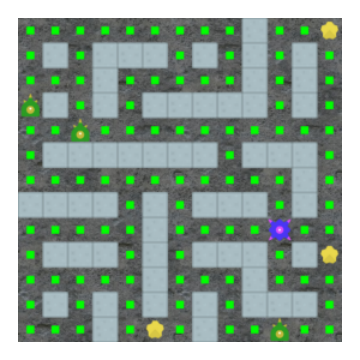
We used 5 tasks from the Procgen (Cobbe et al. 2019, procgen,) suite, shown at Figure 7. We used the default settings for the environments and we only varied the number of training levels used for learning, which we term #levels. The tasks are generally partially-observed (POMDPs) specified by:

1.

Observation space, $\mathcal{O}$ : The original $64\times 64$ RGB pixel-observations, i.e., $o_{t}\in\left[0,1\right]^{64\times 64\times 3}$ .
2.

Action space, $\mathcal{A}$ : The original 15 discrete actions, i.e., $a_{t}\in\{0,\ldots,14\}$ .

A.1.3 MinAtar (Young & Tian 2019)

We used all 5 tasks from the MinAtar (Young & Tian 2019, minatar,) suite, shown in Figure 8, with the default settings. The tasks are fully-observed and specified by:

1.

State space, $\mathcal{S}$ : The original $10\times 10\times\texttt{n\_channels}$ symbolic observations, i.e., $s_{t}\in\left[0,1\right]^{10\times 10\times\texttt{n\_channels}}$ , where n_channels varies between tasks, from $4$ to $10$ .
2.

Action space, $\mathcal{A}$ : The original 6 discrete (non-minimal) actions, i.e., $a_{t}\in\{0,\ldots,5\}$ .
3.

Transition dynamics, $p(s^{\prime}|s,a)$ : The default $0.1$ probability for sticky actions is used.

A.1.4 DeepMind Continuous Control (Tunyasuvunakool et al. 2020)

We use the walker walk task from the DeepMind Continuous Control (Tunyasuvunakool et al. 2020) suite and modified its reward function. Pixel-observations are used, and the problem is generally partially-observed. The task is specified by:

1.

Observation space, $\mathcal{S}$ : A $64\times 64$ RGB pixel-observation, where the robot body is in the centre of the frame, i.e., $o_{t}\in\left[0,1\right]^{64\times 64\times 3}$ .
2.

Action space, $\mathcal{A}$ : A six-dimensional continuous action, i.e., $a_{t}\in\left[-1,+1\right]^{6}$ .
3.

Reward function, $r(s,a)$ : Originally, the reward is bounded in $[0,1]$ , i.e., $r_{t}\in[0,1]$ , which is computed based on the robot’s torso height and forward velocity. We modify the original per-step reward, by setting to zero any reward below a parameter $\eta$ , i.e., $\tilde{r}_{t}=\mathcal{H}(r_{t}-\eta)r_{t}$ , where $\mathcal{H}$ is the Heaviside step function. For $\eta=0$ , we recover the original reward, and for $\eta>0$ we obtain an increasingly more difficult, in terms of exploration, walker task.

Figure 9: walker

A.2 Experiments

In this section, we provide details on the experimental protocol we follow for each experiment.

A.2.1 Figures 1 and 10

We focus on the prediction problem (Sutton & Barto 2018), modelled as a Markov reward process (MRP) with an one-dimensional state space, i.e., $s\in\mathcal{S}=[-3,+3]$ and a discount factor $\gamma=0.9$ . We are provided with state-value target pairs, i.e., $\{(s_{i},\bar{v}_{i})\}_{i=1}^{N}$ with $N=10$ and learn (i) a representation function $\hat{h}(s;\omega)$ , (ii) a value function $\hat{v}(z;\phi)$ and (iii) a model $\hat{m}(\cdot,\cdot|z;\theta)\triangleq(\hat{r}(z;\theta),\hat{p}(z;\theta))$ , represented as neural networks with parameters, $\omega$ , $\phi$ and $\theta$ , respectively. In particular:

$\displaystyle\hat{h}_{\omega}(s)=\hat{h}(s;\omega)$	$\displaystyle=\texttt{tanh}(\text{MLP}_{\omega}(s))\triangleq z\in[-1,+1]^{32}$	(8)
$\displaystyle\hat{v}_{\phi}(z)=\hat{v}(z;\phi)$	$\displaystyle=\text{MLP}_{\phi}(z)\triangleq v\in\mathbb{R}$	(9)
$\displaystyle\hat{p}_{\theta}(z)=\hat{p}(z;\theta)$	$\displaystyle=\text{LSTM}_{\theta}(z,\mathbf{0})\triangleq z^{1}\in[-1,+1]^{32}$	(10)
$\displaystyle\hat{r}_{\theta}(z)=\hat{r}(z;\theta)$	$\displaystyle=\text{MLP}_{\theta}(z)\triangleq r^{1}\in\mathbb{R},$	(11)

where all the multi-layer percepetrons (MLPs) have one hidden layer of 32 units with an ELU (Clevert et al. 2015) non-linearity and $z^{k}$ is the (latent) state after taking $k$ steps with the model $\hat{m}$ , starting from state $z^{0}\triangleq z$ (Silver et al. 2017).

We make value prediction by repeatedly applying the $\hat{m}$ model-induced Bellman operator $\mathcal{T}_{\hat{m}}$ on the value function $\hat{v}$ , i.e., constructing different $k$ -steps model predicted values ( $k$ -MPVs, Eqn. (5)). In particular, the predictions are given by:

$\displaystyle\hat{v}_{\hat{m}}^{0}(s)$	$\displaystyle=(\mathcal{T}_{\hat{m}_{\theta}})^{0}\hat{v}_{\phi}(\hat{h}_{\omega}(s))=\hat{v}_{\phi}(\hat{h}_{\omega}(s))=\hat{v}_{\phi}\circ\hat{h}_{\omega}(s)$	(12)
$\displaystyle\hat{v}_{\hat{m}}^{1}(s)$	$\displaystyle=(\mathcal{T}_{\hat{m}_{\theta}})^{1}\hat{v}_{\phi}(\hat{h}_{\omega}(s))=\left(\hat{r}_{\theta}+\gamma\hat{v}_{\phi}\right)\circ\hat{p}_{\theta}\circ\hat{h}_{\omega}(s)$	(13)
$\displaystyle\hat{v}_{\hat{m}}^{2}(s)$	$\displaystyle=(\mathcal{T}_{\hat{m}_{\theta}})^{2}\hat{v}_{\phi}(\hat{h}_{\omega}(s))=\left(\hat{r}_{\theta}+\gamma(\hat{r}_{\theta}+\gamma\hat{v}_{\phi})\circ\hat{p}_{\theta}\right)\circ\hat{p}_{\theta}\circ\hat{h}_{\omega}(s)$	(14)
	$\displaystyle\;\;\vdots$
$\displaystyle\hat{v}_{\hat{m}}^{k}(s)$	$\displaystyle=(\mathcal{T}_{\hat{m}_{\theta}})^{k}\hat{v}_{\phi}(\hat{h}_{\omega}(s))=\left(\sum_{j=1}^{k-1}\gamma^{j-1}\hat{r}_{\theta}\circ\hskip 1.19995pt\underbracket{(\hat{p}_{\theta}\circ\cdots\circ\hat{p}_{\theta})\hskip 0.0pt}_{j\text{-times}}\ +\ \gamma^{k}\hat{v}_{\phi}\circ\hskip 1.19995pt\underbracket{(\hat{p}_{\theta}\circ\cdots\circ\hat{p}_{\theta})\hskip 0.0pt}_{k\text{-times}}\right)\circ\hat{h}_{\omega}(s)$	(15)

where $\circ$ denotes function composition. Obviously, the $k$ -MPVs with different $k$ have different functional forms, as the predictions at initialisation suggest at Figures 1b and 10a, too. Note that we do not use the bold notation introduced in Eqn. (7) to highlight that there is no Monte Carlo sampling—the learned model is deterministic and the policy is implicit.

We learn the neural network parameters $\omega$ , $\phi$ and $\theta$ using the ADAM (Kingma & Ba 2014) optimiser with decoupled weight decay (Loshchilov & Hutter 2017) to minimise the empirical squared value prediction error for all $k\in\{0,\ldots,10\}$ , i.e.,

\displaystyle\min_{\omega,\theta,\phi}\ \sum_{i=1}^{N}\sum_{k=0}^{K}\|\hat{v}_{\hat{m}}^{k}(s_{i})-v_{i}\|_{2}^{2}.

(16)

The only source of variability between the $k$ -MPVs (implicit value ensemble (IVE) members) is their functional form, induced by different compositions of the learned parametric networks $\hat{v}_{\phi}$ , $\hat{p}_{\theta}$ and $\hat{r}_{\theta}$ as Eqns. (12-15) show.

A.2.2 Figure 3

Data.

We collect experience/data $\mathcal{B}$ by running a uniformly random policy $\pi_{\text{uniform}}$ for $500$ steps (i.e., 25 episodes). We exclude transitions from and to the top left cell, which we call the out-of-distribution (OOD) or unvisited state.

Value learning.

We learn a tabular action-value function $\hat{q}\approx q^{\pi_{\text{uniform}}}$ using expected SARSA (Van Seijen et al. 2009) and then we induce a (state-)value function, i.e., $\hat{v}(s)\triangleq\mathbb{E}_{a\sim\pi_{\text{uniform}}}[\hat{q}(s,a)],\forall(s,a)\in\mathcal{S}\times\mathcal{A}$ .

Model learning.

Maximum-likelihood estimation (MLE, see Section 2) with data $\mathcal{B}$ is used for learning the tabular model of the environment $\hat{m}\approx m^{*}$ .

Visualisations.

The mean and standard deviations are normalised in $[0,1]$ , i.e., for given quantity $x_{s}$ for state $s$ and $x_{\text{min}}$ ( $x_{\text{max}}$ the minimum (maximum) quantity across all states, we plot $\bar{x}_{s}=(x_{s}-x_{\text{min}})/(x_{\text{max}}-x_{\text{min}})$ . We report the results for a single repetition of the experiment since it is a qualitative observation.

IVE( $n$ ).

We calculate the MPVs exactly, according to Eqn. (5). We vary the parameter $n$ , i.e., maximum number of applications of the model-induced Bellman operator $\mathcal{T}_{\hat{m}}$ on the learned value function $\hat{v}$ .

EVE( $n$ ) and EMVE( $n$ ).

The explicit value ensemble (EVE, Figure 2a) and explicit model value ensemble (EMVE, Figure 2b) are also trained on the same data using the same value and model learning algorithms. The ensemble components different only in their (random) initialisation and seed used in stochastic gradient descent.

A.2.3 Table 1

We use the walker task and train Dreamer (Hafner et al. 2019a) for 1M steps. An action repeat of $2$ is used thus 0.5M agent-environment interaction steps are made per run. We repeat each experiment 3 times, varying the random seed in each one. We report the episodic returns (rounded to the nearest tenth) at the end of training by setting the agents in “evaluation” mode and average their performance across 10 episodes.

A.2.4 Figure 4

We train Muesli (without any modification to its acting strategy or learning algorithm) for $100$ M environment frames. Figure 4 (left) reports the final performance of the agent evaluated on an additional 10M frames on the train and test levels. Mean episode returns are normalised as: $\tilde{R}=(R-R_{\text{min}})/(R_{\text{max}}-R_{\text{min}})$ , using min and max scores for each game (Cobbe et al. 2019).

The model-value self-inconsistency, reported in Figure 4 (right), is computed by unrolling the model for $5$ steps using actions sampled from the policy and taking the standard deviation over the IVE:

	$\displaystyle k\text{-MVP}(s)$	$\displaystyle=\mathbf{\hat{v}_{\hat{m}}^{k}}(s)\overset{(\ref{eq:mc-estimator})}{=}\sum_{i=1}^{k-1}\gamma^{i-1}\mathbf{r_{\hat{m}}^{i+1}}+\gamma^{k}\hat{v}(\mathbf{s_{\hat{m}}^{k}})$		(17)
	$\displaystyle\sigma\text{-IVE}(s)$	$\displaystyle=\text{std}_{k}[k\text{-MVP}(s)],\ \text{for }k=1,\dots,5$		(18)

where the “bold” notation refers to reward and value predictions given a single action sequence sampled from the policy $\pi$ , as described in Eqn. (7).

A.2.5 Figure 5

For training the values and model and calculating IVE and EVE, we follow the same protocol as in Figure 3. In this experiment, we use the learned action-value functions instead of the state-values, see Section C.2 for a formal discussion. We denote with $\sigma$ -IVE( $5$ ) and $\sigma$ -EVE( $5$ ) the standard deviation across the $5$ ensemble members of the implicit and explicit ensembles of the action-values, respectively. Also, $\sigma$ -IVE( $5$ ) $\in\mathbb{R}^{\mathcal{S}\times\mathcal{A}}$ and $\sigma$ -IVE( $5$ ) $[s,a]$ is the standard deviation of the implicit value ensemble at the state $s$ for action $a$ . We use the standard deviation across the ensemble of action-values for inducing policies that are novelty- seeking or avoiding:

•

In Figure 5a, the action that maximises the standard deviation across the value ensemble is selected, per-state, i.e., $\pi_{\text{seeking}}(s)=\argmax_{a\in\mathcal{A}}\sigma\text{-XVE}(5)[s,a]$ , where XVE $\in\{$ IVE, EVE $\}$ . These are the novelty-seeking policies that their probability of reaching the novel state is higher than a uniformly random policy.
•

In Figure 5b, the action that minimises the standard deviation across the value ensemble is selected, per-state, i.e., $\pi_{\text{avoiding}}(s)=\argmin_{a\in\mathcal{A}}\sigma\text{-XVE}(5)[s,a]$ , where XVE $\in\{$ IVE, EVE $\}$ . These are the novelty-avoiding policies that their probability of reaching the novel state is lower than a uniformly random policy.

We calculate the probabilities by constructing a Markov chain, induced by the coupling of the policy under consideration $\pi$ and the “true” environment model, $m^{*}$ . The Markov chain’s transition kernel is given by $p_{m^{*}}^{\pi}(s^{\prime}|s)\triangleq\sum_{a\in\mathcal{A}}p_{m^{*}}(s^{\prime}|s,a)\pi(a|s)$ . We can write the transition kernel as a matrix $P_{m^{*}}^{\pi}\in\mathbb{R}^{\mathcal{S}\times\mathcal{S}}$ , such that $P_{m^{*}}^{\pi}[i,j]=p_{m^{*}}^{\pi}(j|i)$ . The $(i,j)$ entry of the transition matrix, i.e., $P_{m^{*}}^{\pi}[i,j]$ is the probability of reaching the state $j$ after one-step when starting from state $i$ and following policy $\pi$ in the environment with model $m^{*}$ . The $(i,j)$ entry of the $l$ -th power of the transition matrix, i.e., $(P_{m^{*}}^{\pi})^{l}[i,j]$ is the probability of reaching the state $j$ after $l$ -steps when starting from state $i$ and following policy $\pi$ in the environment with model $m^{*}$ .

In Figure 5, we start from the bottom right cell, i.e., $i=\texttt{bottom right}$ and plot the probability of reaching the top left cell, i.e., $j=\texttt{top right}$ after $l$ -steps, and we vary $l$ from $1$ to $150$ . We repeat each experiment 100 times, varying the random seed in each one.

A.3 Table 2

We use the minatar tasks and train VPN (Oh et al. 2017) and some variants of it for 2M steps. The only modification to the original VPN(5) is the way value estimates are constructed:

•

$\hat{v}_{\hat{m}}^{1}$ is VPN variant that uses the $1$ -MPV for value estimation.
•

$\hat{v}_{\hat{m}}^{5}$ is VPN variant that uses the $5$ -MPV for value estimation.
•

$\mu$ -IVE( $5$ ) is the original VPN(5) agent that uses the mean over the implicit value ensemble with $n=5$ for value estimation.

The estimated values are used for value-based planning, as discussed in (Oh et al. 2017, Eqn. (1) & Appendix D.).

Appendix B Implementation Details

For our experiments we used Python (Van Rossum & Drake Jr 1995). We used JAX (Bradbury et al. 2018; Babuschkin et al. 2020) as the core computational library for implementing Muesli (Hessel et al. 2021) and VPN (Oh et al. 2017). We used the official TensorFlow (Abadi et al. 2016) implementation of Dreamer (Hafner et al. 2019a). We also used Matplotlib (Hunter 2007) for the visualisations.

B.1 Tabular Methods

We initialise the rewards, transition logits and action-values by sampling from a normal distribution with mean $0$ and standard deviation $1$ . The ADAM (Kingma & Ba 2014) optimiser with learning rate $5e\text{-}5$ is used, and all losses converge after $10,000$ epochs of stochastic gradient descent with batch size $128$ .

B.2 Dreamer (Hafner et al. 2019a)

We use the Dreamer agent’s default hyperparameters, as introduced by (Hafner et al. 2019a). For the self-inconsistency-seeking variant, i.e., $\mu+\sigma$ -IVE(5), we used a scalar weighting factor $\beta_{\text{IVE}}^{*}=0.1$ to balance the mean and standard deviation across the ensemble members, tuned with grid search in $\{0.05,0.1,0.2,1.0,10.0\}$ . The same tuning procedure is used for the baselines. The reported scores are for $\beta_{\text{EVE}}^{*}=0.2$ and $\beta_{\text{EMVE}}^{*}=0.1$ .

B.3 Muesli (Hessel et al. 2021)

We use the Muesli agent’s hyperparameters. In particular we use the ones from the large-scale Atari experiments by Hessel et al. 2021. Nonetheless, we set the fraction of replay data in each batch to $0.8$ (instead of the original $0.95$ ) to shorten training time. To encourage diversity in value and reward predictions for unvisited states we have augmented the value and reward prediction heads of the model with untrainable randomized prior networks (Osband et al. 2018), using a prior scale of $5.0$ . Note that unlike in Osband et al. 2018, we did not introduce additional heads per prediction or modify the training procedure.

B.4 VPN (Oh et al. 2017)

We use the MinAtar DQN-torso (Young & Tian 2019) and an LSTM (Hochreiter & Schmidhuber 1997) with 128 hidden units and otherwise follow the original VPN(5) hyperparameters, as introduced by Oh et al. 2017.

Appendix C Extensions

C.1 IVE with the Bellman Optimality Operator

In Section 3, we defined the $k$ -steps model-predicted value ( $k$ -MPV) in terms of the model-induced Bellman evaluation operator and a value function for a policy $\pi$ , and constructed the implicit value ensemble (IVE) accordingly. In this section. we provide a brief presentation of MPVs and IVE in terms of the model-induced Bellman optimality operator and optimal value functions.

Definition 2 (Bellman optimality operator).

Given the model $m^{*}$ , the one-step Bellman optimality operator $\mathcal{T}^{*}:\mathbb{V}\rightarrow\mathbb{V}$ is induced, and its application on a state-function $v\in\mathbb{V}$ , for all $s\in\mathcal{S}$ , is given by

\displaystyle\mathcal{T}^{*}v(s)\triangleq\max_{a\in\mathcal{A}}\mathbb{E}_{m^{*}}\left[R_{0}+\gamma v(S_{1})\mid S_{0}=s.A_{1}=a\right].

(19)

The $k$ -times repeated application of an one-step Bellman optimality operator gives rise to the $k$ -steps Bellman optimality operator,

\displaystyle(\mathcal{T}^{*})^{k}v\triangleq\hskip 1.19995pt\underbracket{\mathcal{T}^{*}\ldots\mathcal{T}^{*}\hskip 0.0pt}_{k\text{-times}}v.

(20)

The Bellman optimality operator, $\mathcal{T}^{*}$ , is a contraction mapping (Puterman 2014), and its fixed point is the value of the optimal policy $\pi^{*}$ , i.e., $\lim_{n\rightarrow\infty}(\mathcal{T}^{*})^{n}v=v^{\pi^{*}}\triangleq v^{*}$ , for any state-function $v\in\mathbb{V}\triangleq\{f:\mathcal{S}\rightarrow\mathbb{R}\}$ .

Model-induced Bellman optimality operator.

A model $\hat{m}$ induces a Bellman optimality operator $\mathcal{T}_{\hat{m}}^{*}$ with a fixed point $v_{\hat{m}}^{*}$ , i.e., the value of the optimal policy under the model (a.k.a. the solution of the model. Similar to Eqn. (20), a $k$ -steps model-induced Bellman optimality operator is given by $(\mathcal{T}_{\hat{m}}^{*})^{k}v=\hskip 1.19995pt\underbracket{\mathcal{T}_{\hat{m}}^{*}\ldots\mathcal{T}_{\hat{m}}^{*}\hskip 0.0pt}_{k\text{-times}}v$ .

Model-predicted values.

The $k$ -steps MPV, using the model-induced Bellman optimality operator is given by

\displaystyle\hat{v}_{\hat{m}}^{k}\triangleq(\mathcal{T}_{\hat{m}}^{*})^{k}\hat{v}

(21)

Implicit value ensemble.

An ensemble of $k$ -MPV predictions can be made by varying $k$ , giving rise to

\displaystyle\{\hat{v}_{\hat{m}}^{i}\}_{i=0}^{n}\triangleq\hskip 1.19995pt\underbracket{\{\hat{v},\mathcal{T}_{\hat{m}}^{*}\hat{v},\ldots,(\mathcal{T}_{\hat{m}}^{*})^{n}\hat{v}\}\hskip 0.0pt}_{n+1\text{ value estimates}}.

(22)

The IVE with the Bellman optimality operator can be used for values learned with, e.g., Q-learning (Watkins & Dayan 1992), or with other value-based agents, e.g., VPN (Oh et al. 2017). We use this idea in Appendix D.

C.2 MPV with Action-Value Functions

In order to be able to modulate action selection using the self-inconsistency signal, we have computed the k-MPV conditioned on both state and action:

\displaystyle k\text{-MVP}(s,a)

\displaystyle=\mathbf{\hat{q}_{\hat{m}}^{k}}(s,a)=\sum_{i=0}^{k-1}\gamma^{i}\mathbf{r_{\hat{m}}^{i+1}}+\gamma^{k}\hat{v}(\mathbf{s_{\hat{m}}^{k}}),

(23)

where now reward and value predictions are computed after unrolling the model using action $a$ for one step, and actions sampled from the policy for the remaining $k-1$ steps.

Appendix D Additional Experiments

D.1 Measuring Self-Inconsistency in OOD States

To complement our results in Figure 4, we have also evaluated self-inconsistency by computing the IVE as an average over 100 action sequences sampled from the policy, see Figure 11. We observed only minor quantitative differences compared to the results presented in Figure 4 (where we were using a single action sequence to estimate the IVE).

Figure 11:

\sigma

-IVE(

5

) computed using the model of the Muesli agent while evaluating on both training and unseen test levels, for different numbers of unique levels seen during training. To estimate the IVE, we used 100 action sequences from the policy. Bars, error-bars show mean and standard error across 3 seeds, respectively.

D.2 Measuring Explicit Ensemble (EVE) Variance in OOD States

To complement our results in Figure 4 for IVE, we provide the EVE results in Figure 12. We observe that EVE behaves similar to IVE in terms of ensemble variance as a function of #levels for both training and testing levels.

Figure 12:

\sigma

-EVE(

5

) computed using the Muesli agent augmented with an ensemble of 5 value heads (different random initialisation) while evaluating on both training and unseen test levels, for different numbers of unique levels seen during training. (Left:) Performance for training (green) and test (pink) for varying number of levels. (Right:) Explicit value ensemble inconsistency measured by standard deviation of the 5 different heads. Results are from a single seed.

D.3 How to Use the IVE(5) Signal?

In the following experiments we consider the self-inconsistency signal as an optimistic bonus to encourage better exploration during training, hence generalising better during evaluation. We test variants of the $+\sigma$ -IVE(5) signal by mixing the policy with the self-inconsistency in probability space $+\sigma$ -IVE(5) $\triangleq(1-\beta)\pi+\beta\cdot\sigma$ -IVE(5), and by mixing the signal with the policy logits: $z+\sigma$ -IVE(5) $\triangleq\text{softmax}(z_{\pi}+\beta\cdot\sigma$ -IVE(5) $)$ . We vary the number of MPV in the ensemble for $n=5,10$ . Use further test using a different metric for measuring the disagreement across the nMPVs that considers different weighting averages over $k$ :

\displaystyle d_{JS}=\textsc{JSD}_{\mathbf{w}}(\text{IVE}(n))=\textsc{H}\left(\sum_{k}w_{k}\hat{v}^{k}_{\hat{m}}\right)-\sum_{k}w_{k}\textsc{H}\left(\hat{v}^{k}_{\hat{m}}\right)

(24)

with three weighting schemes: a decreasing weight $dec_{JS}:w_{k}=r^{k}/(\sum_{j}r^{j})$ such that the weight decreases to $1/3$ over $n$ , an increasing weight $inc_{JS}$ with the inverse trend, and a uniform weight $uni_{JS}$ that corresponds to the uniform mixing over n $w_{k}=1/n$ .

In Figure 13b we observe that learning with an optimistic bonus helps with generalisation at evaluation time. Figure13c we observe that mixing over probability space is less sensitive to re-scaling $\beta$ , but yields higher variance. We notice a trade-off between the weighting scheme used vs. the size of the IVE, for higher ns the best performing metric has less weight on the larger k-MPVs. For the decreasing metric the results remain more robust, suggesting that the inconsistencies are higher for larger ks. We used $\beta=0.1$ for mixing in probability and $\beta=1$ for the logit case.

D.4 Ablation on Pessimism for Evaluation

We evaluate in Figure 14 how sensitive the self-inconsistency signal is to different re-scaling parameters $\beta$ when acting pessimistically at test time $z-\beta\ d$ - $\sigma$ -IVE(5) with an increasing weight. We trained a vanilla Muesli agent using 10/100 levels over 150M frames and evaluated with a pessimistic bonus for the consecutive 20M frames over 3 seeds.

D.5 Dreamer Variants

In Section 4.2, we modified the Dreamer (Hafner et al. 2019a) agent to improve its exploration without having to learn an explicit ensemble of value functions. We modify the behavioural policy used for collecting data, using the mean and standard deviation of the implicit value ensemble, i.e., $\mu$ -IVE( $5$ ) and $\sigma$ -IVE( $5$ ), respectively. We use the original Dreamer setup otherwise.

In particular, for each time-step $t$ , we sample action $\mathbf{a}_{\pi}^{t}$ from the learned policy $\pi$ and then calculate the IVE( $5$ ), similar to Eqn. (7). Then, we can form the utility function

\displaystyle\mathcal{U}=\mu\text{-IVE}(5)+\beta\cdot\sigma\text{-IVE}(5).

(25)

We use online gradient-based or sample-based planning, a.k.a. model-predictive control (Garcia et al. 1989, MPC,) for selecting an action.

We used $\beta=0.1$ , 10 gradient steps or 10 samples from the learned policy for guiding the search in all of our experiments, shown in Table 3.

Table 3: Results for the Dreamer agent and IVE variants on a modified version of the walker task with varying degrees of reward sparsity controlled by

\eta

, where higher

\eta

corresponds to harder exploration. A “

\diamondsuit

” indicates methods that use gradient-based trajectory optimisation, while “

\clubsuit

” indicates methods that use sample-based trajectory optimisation. We report mean and standard error of episodic returns (rounded to the nearest tenth) over 3 runs after 1M steps. Higher-is-better and the performance is upper bounded by 1000. The best performing method, per-task, is in bold.

Methods	$\eta=0.0$	$\eta=0.2$	$\eta=0.3$	$\eta=0.5$
Dreamer	1000 ${\color[rgb]{0.5,0.5,0.5}\pm 00}$	720 ${\color[rgb]{0.5,0.5,0.5}\pm 10}$	570 ${\color[rgb]{0.5,0.5,0.5}\pm 60}$	80 ${\color[rgb]{0.5,0.5,0.5}\pm 50}$
Dreamer^♢	1000 ${\color[rgb]{0.5,0.5,0.5}\pm 00}$	540 ${\color[rgb]{0.5,0.5,0.5}\pm 30}$	240 ${\color[rgb]{0.5,0.5,0.5}\pm 50}$	40 ${\color[rgb]{0.5,0.5,0.5}\pm 30}$
$\mu$ -IVE(5)^♢	1000 ${\color[rgb]{0.5,0.5,0.5}\pm 00}$	860 ${\color[rgb]{0.5,0.5,0.5}\pm 40}$	690 ${\color[rgb]{0.5,0.5,0.5}\pm 70}$	210 ${\color[rgb]{0.5,0.5,0.5}\pm 60}$
$\mu+\sigma$ -EVE(5)^♢	1000 ${\color[rgb]{0.5,0.5,0.5}\pm 00}$	1000 ${\color[rgb]{0.5,0.5,0.5}\pm 00}$	980 ${\color[rgb]{0.5,0.5,0.5}\pm 10}$	280 ${\color[rgb]{0.5,0.5,0.5}\pm 50}$
$\mu+\sigma$ -EMVE(5)^♢	1000 ${\color[rgb]{0.5,0.5,0.5}\pm 00}$	910 ${\color[rgb]{0.5,0.5,0.5}\pm 20}$	730 ${\color[rgb]{0.5,0.5,0.5}\pm 40}$	210 ${\color[rgb]{0.5,0.5,0.5}\pm 60}$
$\mu+\sigma$ -IVE(5)^♢	1000 ${\color[rgb]{0.5,0.5,0.5}\pm 00}$	1000 ${\color[rgb]{0.5,0.5,0.5}\pm 00}$	1000 ${\color[rgb]{0.5,0.5,0.5}\pm 00}$	330 ${\color[rgb]{0.5,0.5,0.5}\pm 70}$
$\mu+\sigma$ -IVE(5)^♣	1000 ${\color[rgb]{0.5,0.5,0.5}\pm 00}$	1000 ${\color[rgb]{0.5,0.5,0.5}\pm 00}$	1000 ${\color[rgb]{0.5,0.5,0.5}\pm 00}$	280 ${\color[rgb]{0.5,0.5,0.5}\pm 40}$

D.6 Qualitative Analysis of Different Value Ensembles

In Figure 15, we plot the standard deviation across different types of value ensembles, as illustrated in Figure 2.

Appendix E Muesli and its Implicit Value Ensemble

In this section, we provide an exposition of how the (i) functional form and (ii) learning algorithm of the Muesli (Hessel et al. 2021) and MuZero (Schrittwieser et al. 2020) agents contribute to the diversification of their implicit value ensemble (IVE) members. This is to complement our analysis in Section 3.4.

E.1 Functional Form

The Muesli agent (Hessel et al. 2021, see Figure 10,) is comprised of (i) an representation function $\hat{h}(s;\omega)$ , (ii) a (latent) state-value function $\hat{v}(z;\phi)$ and (iii) an action-conditioned model $\hat{m}(\cdot,\cdot|z,a;\theta)\triangleq(\hat{r}(z,a;\theta),\hat{p}(z,a;\theta))$ , represented as neural networks with parameters $\omega$ , $\phi$ and $\theta$ , respectively. We omit the parametrisation and learning of the policy head $\hat{\pi}(\cdot|z)$ since it does not impact our analysis. In summary, the neural network functions are given by:

$\displaystyle\hat{h}_{\omega}(s)=\hat{h}(s;\omega)$	$\displaystyle\triangleq\mathbf{z}\in\mathcal{Z}$	(26)
$\displaystyle\hat{v}_{\phi}(z)=\hat{v}(z;\phi)$	$\displaystyle\triangleq\mathbf{v}\in\mathbb{R}$	(27)
$\displaystyle\hat{r}_{\theta}(z,a)=\hat{r}(z,a;\theta)$	$\displaystyle\triangleq\mathbf{r^{1}}\in\mathbb{R}$	(28)
$\displaystyle\hat{p}_{\theta}(z,a)=\hat{p}(z,a;\theta)$	$\displaystyle\triangleq\mathbf{z^{1}}\in\mathcal{Z}.$	(29)

Note the similarity with Eqn. (8-11). The main difference is that the Muesli’s transition model and reward function, i.e., $\hat{p}_{\theta}$ and $\hat{r}_{\theta}$ , are action-conditioned. We also use the bold notation introduced in Eqn. (7). To ease the analysis, we define the state-to-state transition function and state-to-reward function by coupling the policy $\hat{\pi}$ with the transition function $\hat{p}_{\theta}$ and reward function $\hat{r}_{\theta}$ , respectively, giving rise to a transition and reward kernel i.e.,

	$\displaystyle\mathbf{z^{1}}\sim\hat{p}_{\theta}^{\hat{\pi}}(z)$	$\displaystyle\triangleq\hat{p}_{\theta}(z,\hat{\pi}(\cdot\|z))$		(30)
	$\displaystyle\mathbf{r^{1}}\sim\hat{r}_{\theta}^{\hat{\pi}}(z)$	$\displaystyle\triangleq\hat{r}_{\theta}(z,\hat{\pi}(\cdot\|z)).$		(31)

We construct the implicit value ensemble (IVE) by repeatedly applying the policy $\hat{\pi}$ and $\hat{m}_{\theta}$ model-induced Bellman operator $\mathcal{T}_{\hat{m}_{\theta}}^{\hat{\pi}}$ on the value function $\hat{v}_{\phi}$ , i.e., constructing different $k$ -steps model predicted values ( $k$ -MPVs, Eqn. (5)), given by

$\displaystyle\mathbf{\hat{v}_{\hat{m}}^{0}}(s)$	$\displaystyle=(\mathcal{T}_{\hat{m}_{\theta}}^{\hat{\pi}})^{0}\hat{v}_{\phi}(\hat{h}_{\omega}(s))=\hat{v}_{\phi}(\hat{h}_{\omega}(s))=\hat{v}_{\phi}\circ\hat{h}_{\omega}(s)$	(32)
$\displaystyle\mathbf{\hat{v}_{\hat{m}}^{1}}(s)$	$\displaystyle=(\mathcal{T}_{\hat{m}_{\theta}}^{\hat{\pi}})^{1}\hat{v}_{\phi}(\hat{h}_{\omega}(s))=\left(\hat{r}_{\theta}^{\hat{\pi}}+\gamma\hat{v}_{\phi}\right)\circ\hat{p}_{\theta}^{\hat{\pi}}\circ\hat{h}_{\omega}(s)$	(33)
$\displaystyle\mathbf{\hat{v}_{\hat{m}}^{2}}(s)$	$\displaystyle=(\mathcal{T}_{\hat{m}_{\theta}}^{\hat{\pi}})^{2}\hat{v}_{\phi}(\hat{h}_{\omega}(s))=\left(\hat{r}_{\theta}+\gamma(\hat{r}_{\theta}^{\hat{\pi}}+\gamma\hat{v}_{\phi})\circ\hat{p}_{\theta}^{\hat{\pi}}\right)\circ\hat{p}_{\theta}^{\hat{\pi}}\circ\hat{h}_{\omega}(s)$	(34)
	$\displaystyle\;\;\vdots$
$\displaystyle\mathbf{\hat{v}_{\hat{m}}^{k}}(s)$	$\displaystyle=(\mathcal{T}_{\hat{m}_{\theta}}^{\hat{\pi}})^{k}\hat{v}_{\phi}(\hat{h}_{\omega}(s))=\left(\sum_{j=1}^{k-1}\gamma^{j-1}\hat{r}_{\theta}^{\hat{\pi}}\circ\hskip 1.19995pt\underbracket{(\hat{p}_{\theta}^{\hat{\pi}}\circ\cdots\circ\hat{p}_{\theta}^{\hat{\pi}})\hskip 0.0pt}_{j\text{-times}}\ +\ \gamma^{k}\hat{v}_{\phi}\circ\hskip 1.19995pt\underbracket{(\hat{p}_{\theta}^{\hat{\pi}}\circ\cdots\circ\hat{p}_{\theta}^{\hat{\pi}})\hskip 0.0pt}_{k\text{-times}}\right)\circ\hat{h}_{\omega}(s)$	(35)

where $\circ$ denotes function composition. Obviously, the functional form of the $k$ -MPVs with different $k$ is different since they compose differently $\hat{m}_{\theta}$ and $\hat{v}_{\phi}$ . For instance, $\mathbf{\hat{v}_{\hat{m}}^{0}}(s)$ uses only $\hat{v}_{\phi}$ , while $\mathbf{\hat{v}_{\hat{m}}^{1}}(s)$ and $\mathbf{\hat{v}_{\hat{m}}^{k}}(s)$ for $k>1$ use both $\hat{m}_{\theta}$ and $\hat{v}_{\phi}$ but not in the same way. Instead, for $k\rightarrow\infty$ , we obtain a purely $\hat{m}_{\theta}$ -based prediction (a.k.a. the fixed point of $\mathcal{T}_{\hat{m}_{\theta}}^{\hat{\pi}}$ ).

For a stochastic policy in Eqn. (31) we sample from the policy $\hat{\pi}(\cdot|z)$ . Hence we obtain stochastic estimates of the $k$ -MPV in Eqn. (35), similar to Eqn. (7). Nonetheless, note that the Muesli model is a deterministic expectation model and hence we do not have to sample from it. Empirically, we found that the impact of using a stochastic policy on the estimation of the IVE members was negligible, see Appendix D. We illustrate the computational graph for the $k$ -MPV in Figure 16.

Figure 16: The computational graph of the implicit value ensemble (IVE) members for the Muesli (Hessel et al. 2021) agent. The action nodes

\{\mathbf{a^{i}}\}_{i=0}^{k-1}

are stochastic nodes from which we sample from the (latent-)state-conditioned policy

\mathbf{a^{i}}\sim\hat{\pi}(\cdot|\mathbf{z^{i}})

E.2 Learning Algorithm

The value and model learning algorithms of Muesli further diversify the IVE member predictions. In our analysis, we consider two distinct cases: (i) when the model and value are trained with on-policy trajectories from $\hat{\pi}$ and (ii) when off-policy trajectories from behavioural policies $\pi_{\beta}$ are used. Note that the learning algorithm of the Muesli agent uses a mix of on- and off-policy trajectories, similar to the LASER agent (Schmitt et al. 2020).

On-policy trajectories.

Provided a sequence of states, actions and rewards, collected from running policy $\hat{\pi}$ in the true environment $m^{*}$ , i.e., $(s_{t:t+T},a_{t:t+T},r_{t:t+T})\sim m^{*}_{\hat{\pi}}$ , we present the targets used for the IVE members for the first state, i.e., $\{\mathbf{v_{\hat{m}}^{k}}(s_{t})\}_{k=0}^{K}$ , where in practice $K=5$ (Hessel et al. 2021). We use the notation from Figure 16. $n$ -step bootstrap value estimates (Sutton 1988) are constructed using $\hat{v}_{\phi}$ and used as value targets $v_{t:t+T-1}^{\text{target}}$ , where

\displaystyle v_{t+i}^{\text{target}}=\sum_{j=1}^{n-1}\gamma^{j-1}r_{t+i+j}+\gamma^{n}\hat{v}_{\phi}(s_{t+i+n})

(36)

and $n=5$ . Alternative methods for constructing value targets, e.g., TD( $\lambda$ ) (Sutton & Barto 2018) could be used, too. The “prediction-target” pairs for the different IVE members for state $s_{t}$ and actions $a_{t:t+T}$ are then given by⁶⁶ 6 We assume that $T-1>K+n$ .

\begin{array}[]{rll}\mathbf{\hat{v}_{\hat{m}}^{0}}(s_{t})=&\mathbf{v^{0}}&\longleftarrow v_{t}^{\text{target}}\\ \mathbf{\hat{v}_{\hat{m}}^{1}}(s_{t})=&\mathbf{r^{1}}+\gamma\mathbf{v^{1}}&\longleftarrow r_{t+1}+\gamma v_{t+1}^{\text{target}}\\ \mathbf{\hat{v}_{\hat{m}}^{k}}(s_{t})=&\sum_{i=1}^{k-1}\gamma^{i-1}\mathbf{r^{j}}+\gamma^{k}\mathbf{v^{k}}&\longleftarrow\sum_{i=1}^{k-1}\gamma^{i-1}r_{t+j}+\gamma^{k}v_{t+k}^{\text{target}},\end{array}

(37)

where the $\longleftarrow$ indicates that an objective function (e.g., L2 loss) is minimised that makes the two sides of the arrow approximately equal. Importantly, Muesli and MuZero ground reward and value predictions independently, or in other words, the $k$ -MPV is trained by minimising the following loss:

\displaystyle\mathcal{L}\triangleq(\mathbf{r^{1}}-r_{t+1})^{2}+\cdots+(\mathbf{r^{k-1}}-r_{t+k-1})^{2}+(\mathbf{v^{k}}-v_{t+k}^{\text{target}})^{2}=\sum_{i=1}^{k-1}(\mathbf{r^{i}}-r_{t+i})^{2}+(\mathbf{v^{k}}-v_{t+k}^{\text{target}})^{2}.

(38)

Eqn. (37) highlight that while all the IVE members are trained to approximate the value of the policy $\hat{\pi}$ , i.e., $\mathbf{\hat{v}_{\hat{m}}^{0}}\approx\mathbf{\hat{v}_{\hat{m}}^{1}}\approx\cdots\approx\mathbf{\hat{v}_{\hat{m}}^{k}}\approx v^{\hat{\pi}}$ , each one is regressed against a different target/estimate of the value, further diversifying the ensemble.

Off-policy trajectories.

Provided a sequence of states, actions and rewards, collected from a behavioural policy $\pi_{\beta}$ interacting with the true environment $m^{*}$ , i.e., $(s_{t:t+T},a_{t:t+T},r_{t:t+T})\sim m^{*}_{\pi_{\beta}}$ , we construct off-policy corrected $n$ -step bootstrap value target $v_{t:t+T-1}^{\text{target}}$ with the Retrace (Munos et al. 2016) algorithm, using $\hat{v}_{\phi}$ .

Next, we define the multi-step action-conditioned model-based reward and value estimates, i.e.,

\displaystyle\mathbf{\hat{r}_{\hat{m}}}(s_{t},a_{t},\ldots,a_{t+k-1})\triangleq\mathbf{\hat{r}_{\hat{m}}}(s_{t},a_{t:t+k-1})\quad\text{and}\quad\mathbf{\hat{v}_{\hat{m}}}(s_{t},a_{t},\ldots,a_{t+k-1})\triangleq\mathbf{\hat{v}_{\hat{m}}}(s_{t},a_{t:t+k-1}),

(39)

where for on-policy actions, i.e., $a_{t:t+k-1}\sim\hat{\pi}$ , we note that $\mathbf{\hat{v}_{\hat{m}}}(s_{t},a_{t:t+k-1})$ is the $k$ -MPV of Eqn. (35). As illustrated in Figure 16, the multi-step action-conditioned reward and value estimates in Eqn. (39) are computed by setting the value of the nodes $\mathbf{a^{0:k-1}}$ to the replayed action sequence $a_{t:t+k-1}$ from the behavioural policy $\pi_{\beta}$ . The learning of the model and value function proceeds as in the on-policy case, obtaining the following “prediction-target” pairs, analogous to Eqn. (37)

\begin{array}[]{ll}\mathbf{\hat{v}_{\hat{m}}}(s_{t})&\longleftarrow v_{t}^{\text{target}}\\ \mathbf{\hat{r}_{\hat{m}}}(s_{t},a_{t})+\gamma\mathbf{\hat{v}_{\hat{m}}}(s_{t},a_{t})&\longleftarrow r_{t+1}+\gamma v_{t+1}^{\text{target}}\\ \sum_{i=1}^{k-1}\gamma^{i-1}\mathbf{\hat{r}_{\hat{m}}}(s_{t},a_{t:t+j-1})+\gamma^{k}\mathbf{\hat{v}_{\hat{m}}}(s_{t},a_{t:t+k-1})&\longleftarrow\sum_{i=1}^{k-1}\gamma^{i-1}r_{t+j}+\gamma^{k}v_{t+k}^{\text{target}},\end{array}

(40)

Eqn. (40) suggests that in the off-policy case, $k$ -MPVs are not trained directly since the sampled sequence of actions that conditions the reward and value predictions does not (necessarily) come from $\hat{\pi}$ . Nonetheless, the multi-step action-conditioned reward and value predictors are the building blocks for constructing the $k$ -MPVs and hence we conjecture that the diversity induced by training these with different targets will lead to diversity in the IVE members too.

Overall, the Muesli agent is trained with both on- and off-policy trajectories. In the case of on-policy trajectories, we showed in Eqn. (37) that that different targets are used for training each IVE member. When off-policy trajectories are used, instead of $k$ -MPVs, model-based multi-step action-conditioned reward and value predictors are trained to regress different reward and value targets for different $k$ . These predictors are used for constructing the IVE members at acting time and hence this diversity at training time can impact the diversity of the IVE members too.

Model-Value Inconsistency as a Signal for Epistemic Uncertainty

Abstract

Keywords:

1 Introduction

2 Background

Definition 1 (Bellman evaluation operator).

2.1 Model-Based Reinforcement Learning

Model-induced Bellman operator.

Model learning principles.

2.2 Epistemic-Uncertainty-Aware Agents

Bayesian agents.

Explicit ensemble methods.

3 Your Model-Based Agent is Secretly an Ensemble of Value Functions

3.1 Implicit Value Ensemble

kk-MPV and nn-step returns.

3.2 Model-Value Inconsistency

3.3 Practical Implementation

Expectation models.

3.4 Diversity in the Implicit Value Ensemble

Functional form.

Muesli learning algorithm.

4 Experiments

Baselines.

Environments.

4.1 Detecting Out-Of-Distribution Regimes with Self-Inconsistency

Tabular.

Deep RL.

4.2 Optimism and Pessimism in the Face of Self-Inconsistency

Tabular.

Deep RL.

4.3 Planning with Averaged Model-Predicted Values

Deep RL.

5 Related Work

Ensemble RL methods.

Model-based RL.

Model-value expansion.

Adapting kk.

Novelty signals.

Self-consistency regularisation.

Implicit NN ensembles.

6 Discussion

Future work.

Acknowledgements.

References

Appendix A Experimental Details

A.1 Environments

A.1.1 Tabular Environment

A.1.2 Procgen (Cobbe et al. 2019)

A.1.3 MinAtar (Young & Tian 2019)

A.1.4 DeepMind Continuous Control (Tunyasuvunakool et al. 2020)

A.2 Experiments

A.2.1 Figures 1 and 10

A.2.2 Figure 3

Data.

Value learning.

Model learning.

Visualisations.

IVE(nn).

EVE(nn) and EMVE(nn).

A.2.3 Table 1

A.2.4 Figure 4

A.2.5 Figure 5

A.3 Table 2

Appendix B Implementation Details

B.1 Tabular Methods

B.2 Dreamer (Hafner et al. 2019a)

B.3 Muesli (Hessel et al. 2021)

B.4 VPN (Oh et al. 2017)

Appendix C Extensions

C.1 IVE with the Bellman Optimality Operator

Definition 2 (Bellman optimality operator).

Model-induced Bellman optimality operator.

Model-predicted values.

Implicit value ensemble.

C.2 MPV with Action-Value Functions

Appendix D Additional Experiments

D.1 Measuring Self-Inconsistency in OOD States

D.2 Measuring Explicit Ensemble (EVE) Variance in OOD States

D.3 How to Use the IVE(5) Signal?

D.4 Ablation on Pessimism for Evaluation

$k$ -MPV and $n$ -step returns.

Adapting $k$ .

IVE( $n$ ).

EVE( $n$ ) and EMVE( $n$ ).