The resource cost of large scale quantum computing

Marco Fellous Asiani

Remerciements

Je tiens tout d’abord à remercier ma directrice de thèse, Alexia Auffèves, ainsi que mon co-directeur de thèse, Robert Whitney pour m’avoir proposé ce sujet de thèse, initialement intitulé ”thermodynamique de l’information quantique” mais que j’ai, grâce à eux, pu orienter d’avantage vers les aspects de scalabilité du calcul, qui m’intéressent tout particulièrement. Je les remercie donc pour la liberté qui fut possible vis à vis des orientations choisies ainsi que pour leur précieuse aide tout au long de ma thèse. I would like to thank Hui Khoon Ng as well for all the help she provided in the aspects of fault-tolerance which are central in this PhD, and without who this PhD wouldn’t have been possible. Je remercie aussi Cyril Branciard qui fut impliqué sur le projet de l’étude énergétique du quantum switch, non détaillé dans ce manuscrit, mais qui est un projet ”annexe” sur lequel j’ai pris beaucoup de plaisir à travailler, en partie grâce à Cyril. De manière générale, merci à l’ensemble de mes encadrants pour leurs conseils et guidance tout au long du déroulement de cette thèse.

Je tiens aussi à remercier tous les protagonistes impliqués dans l’ambiance du département PLUM ainsi que du feu bureau F218 désormais remplacé par le F323, qui aura eu sa période de gloire lors de l’ère pré-covid. Je pense évidemment à Alexandra, Julian, Hippolyte, Augustin, Pierre, Juliette, Smaïl, Noé, Patrice (qui s’est découvert une passion pour la raclette depuis son arrivée en France), ainsi qu’aux membres provenant d’autres départements tels que Guilliam (étant donné ses hautes responsabilités administratives au conseil de laboratoire, j’étais forcé de le mettre dans les remerciements, sous peine de risquer des coupures d’électricité et d’internet dans mon bureau), voir n’étant même pas à l’institut Néel (Marie et Juan vous saurez vous reconnaître). Je garde cependant un souvenir mitigé des parties de civilization V durant lesquelles moultes alliances à mon encontre furent créées (souvent sous l’impulsion d’Alexandra et Marie).

Je remercie également les différents membres du groupe, tels que Maria, Léa, ainsi que les derniers arrivés que j’ai moins eu le temps de connaitre en raison du covid, Bruno, Nicolò, Stephen et Irénée. Merci aussi à Raphaël qui va bientôt commencer sa thèse à la suite d’Hippolyte. Je pense en particulier aux discussions passionnantes que nous avons eu, à savoir si il faut calculer les $\chi$ -matrix à l’ordre 2 ou si bah en fait l’ordre un, franchement ça suffit large. I would also like to give a special thanks to Jing Hao (also a new member of the group), who suffered from my many questions on fault-tolerance when I was learning it. In addition, I take the opportunity to wish good luck to Samyak which will start his PhD this year and that showed us his amazing badminton skills the last time he was there. In return, we showed you the cute little animals we have in the mountains in Grenoble such as ticks that gave us nice ”kisses” during our hiking session. But please, don’t thank me back by showing me cute tigers and snakes if I come to India one day, I prefer those in pictures. Thank you also to Alessandro who is doing an exchange in Grenoble and trying to convince everyone that the Mont Blanc is an Italian Mountain. Fortunately I arrived on time to stop this Italian propaganda ! Enfin, je remercie Yvain Thonnart, Matias Urdampilleta, Tristan Meunier, Benjamin Huard, Olivier Buisson et Vladimir Milchakov qui ont su être disponibles à plusieurs reprises lors de mes questions sur l’électronique classique pour le premier,certains aspects de physique des micro-ondes et des qubits de spins pour les seconds et troisième, et diverses petites questions liées aux réalités expérimentales des qubits supraconducteurs pour les trois derniers. Sans leur aide, cette thèse n’aurait pas pu se dérouler de la même manière. Je remercie aussi mes amis à Paris ainsi que mes parents et ma famille, et bien entendu Laurie qui a été d’un grand soutien tout au long de cette thèse.

To finish those acknowledgements, I think that the two great physicists that are Alice and Bob should be acknowledged for all their contributions in the field of physics. From their groundbreaking discovery in quantum causality, in quantum gravity and their courage to try to do very dangerous experiment, sometimes risking their life by going inside blackholes [1]. I believe that I speak for all the community of physicists to tell them: thank you for all the risk you took for the pure goal of improving humanity’s knowledge.

Merci aux membres du jury d’avoir accepté d’en faire partie.

Short summary

This thesis deals with the problematics of the scalability of fault-tolerant quantum computing. This question is studied under the angle of estimating the resources needed to set up such computers. Now that the first prototypes of quantum computers exist, it is time to start making such estimates. What we call a resource is, in principle, very general; it could be the power, the energy, or even the total bandwidth allocated to the different qubits. However, we focus mainly on the energetic cost of quantum computing within this thesis, although most of the approaches used can be adapted to deal with any other resource.

We first study what is the maximum accuracy a fault-tolerant quantum computer can achieve in the presence of a scale-dependent noise, i.e., a noise that increases with the number of qubits and physical gates present in the computer. Indeed, this regime may violate an assumption behind the central theorem of fault-tolerance: the quantum threshold theorem. This theorem states that the accuracy of algorithms implemented on a quantum computer can be arbitrarily high if they are protected by quantum error correction, if enough physical elements (qubits and gates) are available and if the noise strength is below a certain threshold. Since this last assumption must be satisfied regardless of the number of physical elements in the computer, scale-dependent noise can violate it. In the case where this scale-dependent noise can be expressed as a function of a resource, these estimates allow (i) to estimate the maximum precision that the computer can achieve in the presence of a fixed quantity of this resource (which makes possible to deduce the maximum size of the algorithms that the computer will be able to implement, in order to know if the scale-dependent noise is a real problem) and vice versa (ii) to estimate the minimum quantity of resource allowing to reach a given accuracy. Throughout this thesis, our calculations are based on the concatenated Steane error-correcting code (because it is a theoretically well-documented construction that protects the qubits against an arbitrary error and allows us to make analytical calculations).

In a second study, we generalize these approaches in order to be able to estimate the resource cost of a calculation in the most general case. By asking to find the minimum amount of resources required to perform a computation under the constraint that the algorithm provides a correct answer with a targeted probability, it is possible to optimize the entire architecture of the computer to minimize the resources spent while being sure to have a correct answer with a high probability. We apply this approach to a complete model of fault-tolerant quantum computer based on superconducting qubits. Our results indicate that for algorithms implemented on thousands of logical qubits, our method makes possible to reduce the energetic cost by a factor of 100 in regimes where, without optimizing, the power consumption could exceed the gigawatt. This work illustrates the fact that the energetic cost of quantum computing should be a criterion in itself, allowing to evaluate the scaling potential of a given quantum computer technology. It also illustrates that optimizing the architecture of a quantum computer via inter-disciplinary methods, including algorithmic considerations, quantum physics, and engineering aspects, such as the ones that we propose, can prove to be a powerful tool, clearly improving the scaling potential of quantum computers. Finally, we provide general hints about how to make fault-tolerant quantum computers energy efficient.

Court résumé

Cette thèse traite des questions de mise à l’échelle du calcul quantique tolérant aux fautes. Ces questions sont étudiées sous l’angle de l’estimation des ressources nécessaires à la mise en place de tels ordinateurs: maintenant que les premiers prototypes d’ordinateurs quantiques existent, il est temps de commencer à réaliser de telles estimations. Ce que nous appelons ressource est en principe très général, il pourrait s’agir de la puissance, de l’énergie, ou même de la bande passante totale allouée aux différents qubits. Cependant, nous nous focalisons particulièrement sur le coût énergétique du calcul quantique au sein de cette thèse, bien que la plupart des approches utilisées puissent être adapté pour traiter une quelconque autre ressource.

Nous étudions dans un premier temps quelle est la précision maximale qu’un ordinateur quantique tolérant aux fautes peut atteindre en présence d’un bruit dépendant de l’échelle, c’est à dire un bruit qui augmente avec le nombre de qubits ou de portes physiques présents dans l’ordinateur. En effet, ce régime peut violer une hypothèse derrière le théorème central de la tolérance aux fautes: le théorème du seuil (« quantum threshold theorem ») qui stipule que la précision des algorithmes implémentés sur un ordinateur quantique peut être arbitrairement grande si ils sont protégés par de la correction d’erreur quantique, si suffisamment de qubits et portes physiques sont à disposition, et si le taux de bruit est en dessous d’un certain seuil. Cette dernière hypothèse devant être vérifiée peu importe le nombre d’éléments physiques dans l’ordinateur, un bruit dépendant de l’échelle peut la violer. Dans le cas où ce bruit dépendant de l’échelle peut être exprimé en fonction d’une ressource, ces estimations permettent (i) d’estimer la précision maximale que l’ordinateur peut atteindre en présence d’une quantité fixée de cette ressource (ce qui permet de déduire la taille maximale des algorithmes que l’ordinateur pourra implémenter, afin de savoir si le bruit dépendant de l’échelle est un réel problème) et réciproquement (ii) d’estimer la quantité de ressource minimale permettant d’atteindre une précision donnée. Dans toute cette thèse, nos calculs sont basés sur le code correcteur d’erreur Steane concaténé (car c’est une construction bien documentée théoriquement, permettant de protéger les qubits contre une erreur arbitraire et permettant de faire des calculs analytiques).

Dans un second temps, nous généralisons ces approches afin de pouvoir estimer le coût en ressource d’un calcul dans le cas le plus général. En demandant de trouver la quantité de ressource minimale requise pour effectuer un calcul sous la contrainte que l’algorithme fournisse une réponse correcte avec une probabilité ciblée, il est possible d’optimiser l’intégralité de l’architecture de l’ordinateur permettant de minimiser la dépense en ressource tout en ayant une réponse correcte. Nous appliquons cette démarche à un modèle complet d’ordinateur tolérant aux fautes basé sur des qubits supraconducteurs. Nos résultats indiquent que pour des algorithmes implémentés sur plusieurs milliers de qubits logiques, notre méthode permet de réduire la facture énergétique d’un facteur 100, dans des régimes où sans optimisation la consommation en puissance pourrait dépasser le gigawatt. Ce travail illustre le fait que le coût énergétique du calcul quantique devrait être un critère en soit permettant d’évaluer le potentiel de mise à l’échelle des ordinateurs quantiques. Il illustre aussi que l’optimisation de l’architecture d’un ordinateur quantique, via des méthodes transversales, incluant les aspects algorithmiques, de physique quantique, et d’ingénierie, telles que celles que nous proposons, peut se révéler être un outil puissant permettant d’améliorer grandement le potentiel de mise à l’échelle. Enfin, nous donnons des premières pistes permettant de savoir comment réaliser des ordinateurs quantiques économes en énergie.

Introduction

General context of this thesis

In recent years, quantum technologies have grown in interest. This is part of the context of the second quantum revolution, which follows the first one that occurred in the last century. When physicists understood that classical physics was only an approximation of more fundamental quantum laws describing our world: quantum mechanics, they used this knowledge in order to design new technologies such as computers, lasers, solar cells, allowing us to enter in the information age. While quantum mechanics was necessary to design those devices, physicists did not really ”engineer” the quantum effects to create the technology. Instead, they took those effects the way they already existed in nature and directly tried to create devices with those.

The goal of the second quantum revolution is to go beyond this limitation and to design new devices whose working principle would strongly rely on the engineering of all the fundamental quantum effects, such as superposition and entanglement [2, 3]. It relies on having the ability to manipulate individual quantum particles. This is becoming possible because in the last $20$ to $30$ years, experiments showing the possibility to control individual quantum particles with a high level of control have been shown experimentally [4, 5, 6]. The second quantum revolution thus opens possibilities of technological innovations in a wide range of domains. We can think about quantum sensing [7, 8], quantum cryptography [9, 10], quantum communication [11, 12], and of course, what is at the heart of this PhD, quantum computing.

The ultimate goal of quantum computing is to build large-scale quantum computers as they would have a computational power order of magnitudes bigger than today’s best supercomputers for some computational tasks. Because of their very high computational power, quantum computers could impact the national and industrial sovereignty [13]. One example clearly showing it is the Shor factoring algorithm which allows factorizing an integer into prime numbers exponentially faster than the best-known classical algorithm. It would allow breaking RSA encryption protocol that is currently used in the banking and military communications¹¹ 1 The example of Shor is a clear example of the potential exponential speedup in the computing time that quantum computers would have compared to classical supercomputers. We should, however, emphasize that there exist post-quantum cryptography methods [14] which would allow transferring data in a secured manner even against the threat of quantum computers. Also, while quantum computing could be a threat to the standard encryption technique, quantum cryptography would at the same time provide a much more secure way to transmit data such that even quantum computers would not be able to decrypt [9].. A recent estimation considered that with 20 million noisy qubits, it could do this in about eight hours [15] where in comparison, a classical supercomputer could take at least millions of years to do it. Quantum computers already exist today. As an example of that, we can think about the Sycamore quantum processor, which has been associated with a recent claim of quantum supremacy by Google [16]. Other laboratories or companies also have quantum computers, we can think about IBM [17, 18], Intel [19], Rigetti [20] to give a few examples. Actually, the first experimental implementation of a quantum algorithm goes back to the year 1998, when the Deutsch-Jozsa algorithm was implemented on a two qubits quantum computer [21]. However, all those examples are computers of very modest size, containing less than a hundred noisy physical qubits. In order to reach all the potential of the quantum speedup, there is a need to scale up the devices to make large-scale quantum computers.

Many challenges have to be solved to make large-scale quantum computers a reality. One of the main issues is related to the fact that quantum information is very fragile. The qubits are very sensitive to environmental noise, which can modify their state. If it occurs, the answer provided by the algorithm would not be trustable. The intrinsic fragility of quantum information has been seen for some time as a real threat, making quantum computers seen as an unreachable goal [22]. To face this issue, strategies such as quantum error correction and fault-tolerance have been developed. To explain the difference between those concepts briefly, quantum error correction consists in developing algorithms that, if implemented perfectly (i.e., if the gates applied on the qubits during the error correction are ideal) can detect and correct errors occurring on the qubits during the calculation. Fault-tolerance takes into account the fact that error correction is unfortunately a noisy process, and provides explicit circuits allowing to implement error correction in such a way that despite the fact it is a noisy process, because correction is performed, the net effect is an improvement in the protection of the encoded information. Thanks to those protocols, the quantum information can, in principle, be preserved for a long enough time in order to get a trustable answer at the end of the algorithm. A central theorem guaranteeing this is the quantum threshold theorem [23, 24]. It states that if the noise per physical gate is lower than a fixed ”threshold” value, one can regroup multiple physical qubits and gates to create a logical qubit and a logical gate. On a logical level, those elements would do the same operation as their physical counterparts, excepted that because error correction is being performed, everything would be as if the qubits were less noisy. Using enough of those physical elements in a logical element, under the hypothesis that the noise is below a threshold, the noise of qubits and gates on the logical level can be reduced as much as desired. The quantum threshold theorem is a significant result. It guarantees the experimentalists that once they would be able to create good enough physical qubits and implement physical gates in a good enough manner, no further improvement would be necessary from the hardware perspective. Quantum error correction would make the necessary improvements to allow the computer to get to any targetted accuracy. For this reason, this theorem has been a big motivation behind the development of quantum technologies for quantum computing.

However, there are two potential issues with the quantum threshold theorem. The first one is that, because fault-tolerance and error correction require many additional physical qubits and gates to be implemented, we might expect to have a significant overhead in terms of physical components required. The estimations of their number vary, but between hundreds of thousands to potentially billions of qubits might be required to implement a fault-tolerant algorithm showing a clear quantum supremacy [25, 26, 15]. This naturally raises the general question of the resources (energy or power, for instance) that would be required to build such large-scale quantum computers. Given the number of qubits needed, we could naturally expect that the energetic cost of such computers might be high. An even better question to answer would be to see if it is possible to design robust methods allowing to minimize the resources expenses of such computers. The second issue with the quantum threshold theorem is that the physical components must already be of good quality in order to make error correction useful: the noise must be below the threshold, and it must remain below this value even if the computer is composed of the potentially billions of physical qubits required for quantum error correction. This can be very challenging as having a well-controlled environment is much easier when the number of qubits is low than when many qubits are inside the computer. The work done in this Ph.D. focuses on those problems.

Positioning of the present Ph.D. work

In this Ph.D., we are studying the question of the scalability of quantum computing by estimating how much resources it would require. In principle, what we call a resource is very general: it could be energy, power, the total frequency bandwidth allowed for the qubits, etc. Now that quantum computing is becoming a reality, and because we have access to the characteristics of the first noisy prototypes of quantum computers, such estimations can, and should be done in order to design the next generation of quantum computers which are expected to be fault-tolerant.

Our goal in this thesis is first to design a general approach that could be used to estimate the largest algorithms that could be implemented with quantum error correction, assuming a fixed amount of resources available. It is also, reciprocally, to evaluate the minimum amount of resources required to implement a given algorithm.

While our approach is general, we then focus on the energetic cost of large-scale quantum computing. There are two reasons for that. First, the energy (or power) required to run a quantum computer is a ”good variable” to know if an architecture is scalable. This is because energetic quantities encompass many criteria coming from various fields. For instance, a low energetic cost is likely to be associated with a ”reasonable” design from an engineering perspective. The other reason we focus on energy and power is that the energy cost required to create large-scale quantum computers could be considerable. It is essential ”in itself” to know how much energy would be needed to implement concrete algorithms.

For this reason, our ending goal is to try to make an in-depth estimation of the power that would be required to implement algorithms on a superconducting qubit fault-tolerant quantum computer. The reason why we focus on superconducting qubits is because it is one of the most mature technologies used for quantum computers today (many experimental values are accessible). Such qubits must be maintained at very low temperatures, which might require a large amount of cryogenic power. We consider using the Steane quantum error correction code (it is a code that protects qubits against arbitrary single-qubit errors). We implement it fault-tolerantly with the so-called ”concatenated construction”. The concatenated construction is a way to implement the code allowing to reach an arbitrarily high level of protection, assuming the noise is below the threshold initially (it is a construction in which the quantum threshold theorem can be rigorously derived). The reason why we choose such code and fault-tolerant construction is because it is very well documented theoretically, we have access to the concrete circuits allowing us to implement it, and it will enable us to perform analytic calculations, which is a requirement to keep our approach simple to explain.

Finally, the overall philosophy behind our work is to design inter-disciplinary methods allowing us to estimate the amount of resources required by involving characteristics coming from quantum error correction, quantum algorithm, engineering, cryogenics, physics of the quantum gate, etc. A quantum computer being a multi-disciplinary device, inter-disciplinary approaches to the design are necessary, especially to minimize resource expenses. Those methods are mainly provided in the last two chapters of this thesis. They are said to be full-stack as each ”stack” in the quantum computer will be modeled (where for us, a stack can be the physics of the quantum gate, the algorithm implemented, the fault-tolerance construction considered, etc).

Our work in more details

The first question we will investigate is finding the largest algorithm a quantum computer can successfully implement, using quantum error correction in the presence of a scale-dependent noise. A scale-dependent noise is a noise whose strength grows with the number of physical components inside the quantum computer. The connection with resource estimation is that in the presence of a limited amount of resources for all the computer, when scaling up, each of the physical components in the computer will receive a fewer amount of this resource. It will typically induce noisier operations. For instance, for a fixed amount of available frequencies for the qubits, the more qubits there are inside the computer, and the more probable crosstalk issues (i.e., the fact to address extra other qubits than the ones that are targetted by the driving signals) might occur [27, 28]. Many other examples of scale-dependent noise can occur. The general idea is that it might be possible to create qubits in an environment where they experience a low amount of noise, but what is complicated is to maintain this low noise environment when more and more qubits are added [29, 30]. Having a noise that is growing in intensity with the size of the computer is already annoying in itself, but what can be worse is that this condition can violate one crucial hypothesis behind the quantum threshold theorem: the requirement that the noise of the physical component must be below the threshold. Indeed, if the noise grows with the size of the computer, it is possible that while being lower than the threshold for a small number of qubits, it gets higher than this value when all the additional qubits used to perform error correction are included. If it occurs, the accuracy of the computer is then intrinsically limited because either no error correction or only a limited amount of it would be possible. Those issues motivated the work presented in the third chapter of the manuscript. There, we study how to maximize the accuracy of the logical gates in the presence of a scale-dependent noise, allowing us to deduce the largest algorithm the computer would be able to run successfully. From the connection between scale-dependent noise and limited resource we established, we provide a first approach allowing to find the minimum resource required to implement the algorithm, and reciprocally to find what is the maximum accuracy the logical gates of a computer can get to in the presence of a limited fixed amount of resource. However, the approaches developed in this chapter do not allow us to treat any kind of resource optimization.

This is why we investigated further to find a general way to formulate the problem. The first thing to acknowledge is that the question of resource estimation of large-scale quantum computing is a question that is at the frontier of many different disciplines; one cannot only focus on the noise felt by the physical qubits to answer this question. For instance, it requires knowledge from quantum physics but also from computer science, cryogenics, and engineering. One important issue it brings is the almost omnipresence of contradictory behaviors that might intersect all those different fields. To give a few examples, ion trap technologies are associated to a very long lifetime for the qubits. Coherence times about $600s$ [31] and even hours [32] have been reached experimentally. All this while having quantum gates that can last for $100\mu s$ [31], providing the ratio of coherence time divided by the gate duration, which can be close to $10^{6}$ , much higher than in many other technologies [33, 34]. From this perspective, they could be seen as ideal candidates for large-scale, fault-tolerant quantum computers as they would be associated with a low overhead in terms of physical qubit per logical qubit. But on the other hand, there are real challenges putting many ions together in a single trap while guaranteeing good connectivity and high coherence times [31] which is a clear drawback for scalability. This is why strategies consisting of regrouping the ions in smaller groups are considered. However, it introduces other challenges, such as how to move the ions efficiently to implement the appropriate interactions. This is one example of contradictory behaviors or challenges that can cross different fields. If we think about superconducting qubits now, many of them could be put on a small size chip such that they are not facing the issue ion trap are²² 2 Crosstalk issues could occur but in a less problematic way than for ions.. But their lifetime is not comparable to what it is possible to do with ion traps, and those qubits must typically be at very low temperatures, close to $10mK$ [35, 33]. Assuming that a superconducting quantum chip would have many physical qubits, potentially between hundred of thousands and the billion depending on the size of the fault-tolerant algorithm that is supposed to run and the quality of the qubits, it could lead to potential issues concerning the energetic cost. More generally, many other technologies have their pros and cons in terms of scalability, resource cost, and level of maturity. There is quantum computing based on photons (linear optics quantum computation) [36, 37], nuclear magnetic resonance quantum computing [38], quantum computing based on spin qubit, and the list continues. Spin qubits [34] are seen as excellent candidates in terms of scalability as they can benefit from the maturity of CMOS technology in terms of integration [39, 40]. Still, this approach to quantum computing is much more recent and does not benefit yet from the same maturity as superconducting qubits.

Here, we mainly talked about competition phenomena occurring between different fields of science, but they may also arise within a given domain. For instance, it is believed that to scale up superconducting or spin qubits quantum computers, electronics controlling or generating the signals that will implement quantum gates on the qubits should be put inside of the cryostat [41, 42, 43]. But different technologies would allow for that: CMOS technology can be put at cold temperature and can generate signals of good quality, but it is associated with a more important thermal load than other approaches such as superconducting circuits [44, 43] or adiabatic computing [45] (which in return do not have the same level of maturity in term of performances). Choosing ”the best” technology is then not easy. And we mainly talked about what happens for the hardware, but many different solutions can also be chosen on the software side of a quantum computer. For instance, there are many different possible strategies on the quantum-error correction side to consider. Thinking about the various areas of research and strategies to implement quantum error correction, we can give the examples of topological quantum error correction such as the surface code [46, 47], bosonic codes [48, 49, 50], concatenated constructions [23, 51] etc. All the different codes and ways to implement them can be associated with different overheads in terms of the number of physical qubits and performance in reducing the errors. Benchmarking quantum error correction to find which code is the most resource-efficient is a complicated task because of the many different aspects that could be benchmarked. As we said before, even if one code appears to be better than another one from a specific performance in noise reduction, it will not necessarily be the best one when the full quantum computer is considered (if it has good performance in terms of noise reduction but requires very heavy classical processing, it might not be a very good candidate). As we see, quantum computing is a field full of contradictions!

What this discussion illustrates is mainly the fact that inter-disciplinary approaches to the problem of scalability must be considered as all the different components involved in the design of a quantum computer are strongly interconnected. But what would be desirable would be to have a well-defined and unique question to answer that would lead the entire design of the quantum computer. Indeed one issue is also that ”too many” choices are possible in the design of the computer and it is hard to choose the best one. To phrase a ”good” question, we can make the following analysis: even though at first view many elements in the quantum computer seem to be very far from the ”quantum world” (cryogenics or signal generation are good examples), they are actually intrinsically connected to it. Indeed, the ultimate goal of a quantum computer is to provide a trustable answer to some algorithm that has been implemented. The whole design of the quantum computer is made so that this condition must hold. For instance, a cryostat has to be designed because the qubits must be maintained cool, and this is because the quantity of noise felt by the qubits must be kept low to have a successful answer for some algorithm. Thus the design of a cryostat is indirectly connected to algorithmic aspects. Seeing the problem under this angle allows to see that connecting the algorithmic aspect, and more precisely, the probability that the algorithm succeeds to all the engineering involved in the design of a quantum computer can give the appropriate constraint to know how to design the computer. Now, only asking to solve this question might lead to many choices in the design, and many of them might be unreasonable. For instance, if one design will satisfy this condition but will induce a quantum computer consuming hundreds of gigawatts, it will not be a good choice ”for all practical purposes”. This is why one step further is to lead the design by asking to minimize a given resource under the constraint that the algorithm succeeds with a targetted probability. Taking the power consumption as a resource and phrasing the question this way will then provide the appropriate constraints on the design of the quantum computer in such a way that it implements the algorithm successfully (which is its ultimate goal) while spending the least amount of power to do this (which will lead to a ”reasonable” design). The constraints this question gives can then directly guide the engineers, physicists, and computer scientists to design the computer together. In the fourth chapter of this thesis, we will provide the conceptual elements required to apply this method properly. In the last chapter, we are going to use it in a complete model of a quantum computer where we will optimize the amount of error correction to perform, the optimal temperature of the different stages of the cryostat (which contains the qubits but also the electronics generating the signals) and the level of attenuation that is chosen on the driving line³³ 3 As we are going to see, attenuation is being put on the coaxial cable where the signals driving the qubit are injected to reduce the thermal noise. to implement fault-tolerant algorithms involving thousands of logical qubits with a high enough targetted probability of success. We will see that orders of magnitude of power consumption can be gained in regimes, where without our optimization, a power consumption bigger than the gigawatt could be involved. It indicates that our approach can significantly enhance the scalability of the architecture. We will also see how the design of the computer depends on the characteristics of the implemented algorithm: it shouldn’t be surprising that the size of the algorithm and the way it is implemented can impact the optimal design of the computer (and, of course, its energetic cost). Finally, because we are going to find the minimum power required to implement an algorithm, the way we formulate the problem can allow to actually define properly the question of the energetic cost of quantum computing.

Outline of the manuscript

This thesis is organized as follows. The first chapter is dedicated to provide the essential tools we need from circuit quantum electrodynamic theory to understand how noisy gates performed on superconducting qubits are and how much power is required to implement them. We also give the state-of-the-art values for superconducting qubits we will consider using in the rest of the thesis. The second chapter is dedicated to quantum error correction and fault-tolerance. We provide all the theoretical results allowing us to understand this theory. Those two chapters do not contain any original results; they just introduce the tools required to understand the last three chapters.

The third chapter is the first one providing results from this Ph.D. It is dedicated to understand what happens for fault-tolerance when the noise felt by the qubits grows with the number of qubits: what is occurring in this regime, and is it necessarily an issue for scalability. This chapter will also give first intuitions about how it is possible to estimate the minimum resources required to implement a fault-tolerant algorithm as having a scale-dependent noise is often related to resource constraints. The fourth chapter is dedicated to explain precisely the method allowing to find how much resources a calculation requires. More specifically, we will show that the minimum power required and the optimal architecture the quantum computer should have to reach this minimum can be found. The last chapter applies those concepts in a complete model of quantum computer based on superconducting qubits where we do quantitative estimations of the energetic cost required to run different kinds of large-scale algorithms. Our work indicates that the inter-disciplinary approach to the question of energetics we propose can reduce the power consumption of the computer by orders of magnitudes in a regime where the consumption could otherwise be higher than the gigawatt. We will also give some first intuitions about what is essential to optimize to make fault-tolerant quantum computing energy-efficient. This work illustrates that the energetic cost of quantum computing should be a figure of merit by itself on the scorecard of qubits technology to assess their potential for scalability. It also shows that optimizing the architecture of a quantum computer through methods like the one we are proposing can be a powerful tool allowing to clearly improve the potential in terms of scalability.

Chapter 1 Physics of superconducting qubits

In all this Ph.D. thesis, the physical examples we will consider will be based on superconducting qubits. The goal of this chapter is, first, to explain the basics of the physics they rely on. Then, we will explain what is the origin of the noise when they are being manipulated before calculating the energetic cost to perform single-qubit gate operations. We will also give there the characteristics of the qubits and gates we will use along this thesis. This energetic cost is one important building block that we will use in the rest of this Ph.D. thesis. This chapter, apart from the section 1.3.1.1, does not contain any original result; we just provide the tools we need to understand the rest of this thesis.

1.1 Designing superconducting qubits

Our goal here is to explain how to make a superconducting qubit and what is the transmon regime. For this purpose, we need to be able to describe quantum phenomena in electrical circuits. This is usually done through the canonical quantization procedure that we are going to explain. Some references on the subject can be found in [52, 53, 54, 55]. We will then apply this method for the electrical circuits we will consider: we will start by quantizing a simple LC circuit before explaining the quantization of a superconducting qubit. Our explanations are mainly taken from [52].

1.1.1 Quantization of electromagnetic circuits

1.1.1.1 Canonical quantization

One way that is used to quantize a classical theory is called the canonical quantization. But in order to describe it, we need to make a few reminders about Lagrangian and Hamiltonian mechanics.

Basics of Lagrangian and Hamiltonian formulation of classical mechanics

Let us consider a classical system. This system can be described by the mean of its coordinates in the phase space. If one considers a system with $N$ degrees of freedom, its state is entirely described by $N$ coordinates $\{q_{k}\}_{k=1}^{N}$ and associated velocities $\{\dot{q}_{k}\}_{k=1}^{N}$ . A Lagrangian $\mathcal{L}$ is a function $\mathcal{L}(\{q_{k}\}_{k=1}^{N},\{\dot{q}_{k}\}_{k=1}^{N})$ from which the classical equations of motion can be deduced by the mean of the Euler-Lagrange equations [56]:

\displaystyle\forall k\in[|1,n|]:\frac{d}{dt}\frac{\partial\mathcal{L}}{\partial\dot{q}_{k}}=\frac{\partial\mathcal{L}}{\partial q_{k}}.

(1.1)

To fix ideas, we can take the example of a one dimensional mechanical harmonic oscillator. Calling $x$ the relative distance to the rest position, this physical system satisfies the equation of motion

\displaystyle\ddot{x}+\omega_{0}^{2}x=0

(1.2)

where $\omega_{0}$ is the resonant frequency of this oscillator. An appropriate Lagrangian to describe this dynamic would be:

\displaystyle\mathcal{L}(x,\dot{x})=\frac{m}{2}\dot{x}^{2}-\frac{m\omega_{0}^{2}}{2}x^{2}.

(1.3)

This is because applying the Euler Lagrange equation (1.1) in this situation would give:

\displaystyle\frac{d}{dt}\frac{\partial\mathcal{L}}{\partial\dot{x}}=\frac{\partial\mathcal{L}}{\partial x}\Leftrightarrow m\ddot{x}=-m\omega_{0}^{2}x,

(1.4)

which provides the appropriate equation of motion (1.2)¹¹ 1 Actually, many equivalent Lagrangian can describe properly a system [56]. Removing the term $m$ , homogeneous to a mass would for instance, also provide the appropriate dynamic and is thus not strictly necessary. It is only in order to get quantities homogeneous to energy that we considered it here.. We also notice that this Lagrangian has the expression of the kinetic energy of the system minus the potential energy. A valid Lagrangian does not necessarily have this shape, but in many situations, it will occur to be the case [57].

In order to understand the quantization procedure later on, we must also introduce the Hamiltonian formulation of classical mechanics. First, the Lagrangian allows to define the generalized momentum $p_{i}$ associated to any of the generalized coordinate $q_{i}$ :

\displaystyle\forall i\in[|1,n|]:p_{i}\equiv\frac{\partial\mathcal{L}}{\partial\dot{q}_{i}}.

(1.5)

It also allows to define a Hamiltonian for the system through the equation:

\displaystyle H(\{q_{k}\}_{k=1}^{N},\{p_{k}\}_{k=1}^{N})\equiv\sum_{k=1}^{N}\dot{q}_{k}p_{k}-\mathcal{L}(\{q_{k}\}_{k=1}^{N},\{\dot{q}_{k}\}_{k=1}^{N})

(1.6)

The equation of motions in the Hamiltonian formalism can be written as:

		$\displaystyle\forall i\in[\|1,n\|]:\dot{p}_{i}=-\frac{\partial H}{\partial q_{i}}$		(1.7)
		$\displaystyle\forall i\in[\|1,n\|]:\dot{q}_{i}=\frac{\partial H}{\partial p_{i}}$		(1.8)

Those first order differential equations are mathematically equivalent to the second order Euler Lagrange equations (1.1) [56].

Keeping the example of the harmonic oscillator, we would for instance find that the momentum associated to the position $x$ is simply:

\displaystyle p=\frac{\partial\mathcal{L}}{\partial\dot{x}}=m\dot{x}

(1.9)

And the Hamiltonian is:

\displaystyle H(x,p)=\dot{x}p-\mathcal{L}(x,\dot{x})=\frac{p^{2}}{2m}+\frac{m\omega_{0}^{2}}{2}x^{2}

(1.10)

The last concept we will need in order to understand the quantization of a classical theory is the notion of Poisson bracket. Let us consider an arbitrary function $A(\{q_{i}\},\{p_{i}\},t)$ . The equation of motion of this function satisfies:

\displaystyle\frac{dA}{dt}=\sum_{i}\left(\frac{\partial f}{\partial q_{i}}\frac{\partial q_{i}}{\partial t}+\frac{\partial A}{\partial p_{i}}\frac{\partial p_{i}}{\partial t}\right)+\frac{\partial A}{\partial t}

(1.11)

And, using (1.7) and (1.8), it can be rewritten as:

\displaystyle\frac{dA}{dt}=\sum_{i}\left(\frac{\partial A}{\partial q_{i}}\frac{\partial H}{\partial p_{i}}-\frac{\partial A}{\partial p_{i}}\frac{\partial H}{\partial q_{i}}\right)+\frac{\partial A}{\partial t}=\{A,H\}+\frac{\partial A}{\partial t}

(1.12)

Where the Poisson Bracket $\{.,.\}$ is defined in general by:

\displaystyle\{A,B\}\equiv\sum_{i}\left(\frac{\partial A}{\partial q_{i}}\frac{\partial B}{\partial p_{i}}-\frac{\partial A}{\partial p_{i}}\frac{\partial B}{\partial q_{i}}\right)

(1.13)

We notice in particular:

		$\displaystyle\{q_{i},p_{j}\}=\delta_{i,j}$		(1.14)
		$\displaystyle\{q_{i},q_{j}\}=\{p_{i},p_{j}\}=0$		(1.15)

We will see that the structure of the equations of motions in the Hamiltonian formalism, when expressed with the Poisson bracket, are very similar to the equation of motions of operators in the Heisenberg formalism of quantum mechanics. This will be the starting point of the canonical quantization principle.

equation of motion of a quantum system in Heisenberg picture

Now we consider a quantum system described by a Hamiltonian $\widehat{H}$ . We assume that this Hamiltonian is composed of generalized coordinates operators $\{\widehat{q}_{i}\}$ and associated momentum $\{\widehat{p}_{i}\}$ . In the Heisenberg picture of quantum mechanics, the equation of motion of any operator $\widehat{A}_{H}$ acting on S follows the equation:

\displaystyle\frac{d\widehat{A}_{H}(t)}{dt}=\frac{1}{i\hbar}[\widehat{A}_{H}(t),\widehat{H}]+\frac{\partial\widehat{A}_{H}(t)}{\partial t}

(1.16)

The coordinates and momenta satisfy the commutations relations:

		$\displaystyle[\widehat{q}_{i}(t),\widehat{p}_{j}(t)]=i\hbar\delta_{ij}$		(1.17)
		$\displaystyle[\widehat{q}_{i}(t),\widehat{q}_{j}(t)]=[\widehat{p}_{i}(t),\widehat{p}_{j}(t)]=0$		(1.18)

(1.16) and (1.17),(1.18) contain all the information to deduce the behavior of any operator at time $t$ which is a polynome in the variables $\{p_{i}(t)\}$ and $\{q_{i}(t)\}$ .

Quantization procedure

At this point, we can notice the strong similarity between (1.16) and (1.12), and also between (1.17),(1.18) and (1.14),(1.15). Indeed, the quantum equations of motion can be obtained by replacing the Poisson bracket $\{A,B\}$ in those equations by a commutator $\frac{1}{i\hbar}[A,B]$ equal to this Poisson bracket. This will provide the appropriate equation of motion for the operator, as well as define the commutation relations properly. In practice, to obtain the quantum theory, it will be enough to promote the Hamiltonian into an operator by imposing the commutation relations:

		$\displaystyle[\widehat{q}_{i}(t),\widehat{p}_{j}(t)]=i\hbar\delta_{ij}$		(1.19)
		$\displaystyle[\widehat{q}_{i}(t),\widehat{q}_{j}(t)]=0$		(1.20)
		$\displaystyle[\widehat{p}_{i}(t),\widehat{p}_{j}(t)]=0$		(1.21)

Further problems might occur in practice (for instance, if in the classical Hamiltonian terms like $x.p$ appears there is a choice of ordering to take because while $x$ and $p$ commute classically, they don’t commute anymore when promoted into operators), but we will not be facing them in what follows such that we can ignore those issues. This ”resemblance” in the classical and quantum theory has originally been discovered by Dirac in 1925 [56], and the mapping we describe here defines the so-called ”canonical quantization” of a classical theory. This should not be understood as a general proof of how a quantum theory can be deduced from a classical theory but more as a guess which provides a recipe that works for many systems. Indeed, the natural order of things would be to deduce a classical theory from the quantum one, the latter being more fundamental. However, such a procedure will at least work for the class of system we are going to study in this Ph.D.

1.1.1.2 An application: quantum description of an LC circuit

To introduce the concepts we need behind the quantization of electromagnetic circuits, we can start with the LC circuit represented in the figure 1.1.

Refer to caption — Figure 1.1: The LC circuit we are considering

In order to anticipate the usual way superconducting qubits are described, we will introduce a new physical quantity: the generalized flux variable. If we consider a point in the circuit where the electric potential is $V(t)$ , the generalized flux variable is defined as [52]:

\displaystyle\phi(t)\equiv\int_{-\infty}^{t}V(t^{\prime})dt^{\prime}

(1.22)

In all what follows we will also assume that all electrical quantities vanish at $t=-\infty$ . Calling $\phi$ the generalized flux associated to the voltage difference around the inductor, the current in the circuit satisfies $I=\phi/L=-C\ddot{\phi}$ . It gives an equation of motion being, with $\omega_{0}=\frac{1}{\sqrt{LC}}$ .

\displaystyle\ddot{\phi}+\omega_{0}^{2}\phi=0

(1.23)

To quantize the description we will proceed as explained in the section 1.1.1. We consider $\phi$ being our generalized coordinate. A possible Lagrangian describing this dynamic is:

\displaystyle\mathcal{L}(\phi,\dot{\phi})=\frac{C}{2}\dot{\phi}^{2}-\frac{\phi^{2}}{2L}

(1.24)

The conjugated momentum associated to $\phi$ is:

\displaystyle P\equiv\frac{\partial\mathcal{L}}{\partial\dot{\phi}}=C\dot{\phi}

(1.25)

We notice that $C\dot{\phi}$ physically corresponds to the charge on the negative plate of the capacitor. We can deduce the Hamiltonian:

\displaystyle H(\phi,P)\equiv P\dot{\phi}-\mathcal{L}(\phi,\dot{\phi})=\frac{P^{2}}{2C}+\frac{\phi^{2}}{2L}

(1.26)

The canonical quantization principle explained in 1.1.1 tells us that to obtain the quantum theory of this system, we just have to promote $\phi$ and $P$ into operators by imposing the commutation relation:

\displaystyle[\widehat{\phi},\widehat{P}]=i\hbar

(1.27)

We see that our choice of Lagrangian consists in considering the energy stored in the capacitor as kinetic energy (because associated to $P$ ), while the energy stored in the inductor is seen as potential energy. But there is nothing fundamental about that; it simply comes from our choice of choosing $\phi$ as the coordinate. Another approach would have been to choose the charge stored by the capacitor as being the generalized coordinate. In this situation, the interpretation of kinetic and potential energy between inductor and capacitor would have been reversed.

A systematic approach to quantize electrical circuits

In all that follows, the Lagrangian is always going to be written:

\displaystyle\mathcal{L}=\mathcal{E}_{C}-\mathcal{E}_{L},

(1.28)

where $\mathcal{E}_{C}$ corresponds to the energy stored by the capacitive elements of the circuit, and $\mathcal{E}_{L}$ to the inductive ones. The generalized coordinate is always going to be the generalized flux (1.22). A precise definition of capacitive and inductive elements can be found in [52]. In this work, we will only have capacitors, inductors, and Josephson junction (that we are going to introduce). The Josephson junction will be considered as an inductive element, and its associated potential energy is going to be taken into account in $\mathcal{E}_{L}$ . This approach to quantize electrical circuits is the one proposed in [52].

1.1.2 Superconducting qubit and transmon regime

Now that the basic principles of how one can have a quantum description of an electrical circuit have been explained, we are going to see how we can engineer a superconducting qubit in practice and what is the so-called transmon regime.

1.1.2.1 The need for non-linear oscillators

A quantum computer usually requires quantum systems having quantum states living in a two-dimensional Hilbert space: qubits. Ideally, we would like to create a physical system for which the quantum state exactly lives in a bi-dimensional Hilbert space. In the context of superconducting qubits, it is not possible. The strategy is then to create an approximation of a qubit. This is often done by considering a two-dimensional subspace of a physical system of high dimensions.

One way to do it experimentally is to realize a non-linear quantum oscillator. A non-linear quantum oscillator has energy levels that are not equally spaced, as represented in Fig 1.2, in comparison to a harmonic oscillator. The advantage in using such a physical system is that assuming the initial state of the system lives in the Hilbert space spanned by the two lowest energy eigenstates, by sending signals resonant with the associated energy transition, the system will remain in this bi-dimensional subspace.

As we are going to see, designing such systems can be done by replacing the inductor composing the LC oscillator with an element called the Josephson junction that we are now going to introduce.

1.1.2.2 The Josephson junction

A Josephson junction is a two-terminal electric component composed of two superconducting electrodes separated via an insulator. In terms of description, it can be modeled by a capacitor in parallel to a Josephson tunnel element as shown in Figure 1.3. To describe the electrical properties of a Josephson tunnel element, we will use again the generalized flux corresponding to the voltage applied to this element.

Calling $\phi_{J}$ the generalized flux associated to the voltage around the Josephson tunnel element, the electrical equations are:

		$\displaystyle\phi_{J}(t)\equiv\int_{-\infty}^{t}U_{J}(t^{\prime})dt^{\prime}$		(1.29)
		$\displaystyle I_{J}(t)=I_{0}\sin\left(\frac{\phi_{J}(t)}{\varphi_{0}}\right)$		(1.30)
		$\displaystyle\varphi_{0}\equiv\frac{\hbar}{2e}$		(1.31)

$\varphi_{0}$ is called the superconducting flux quantum, $2e$ physically represents the charge of a Cooper pair which are the particle leading to the superconducting current. Typical experimental values for the current $I_{0}$ lie between the $\mu A$ and $nA$ [52].

This element can be seen as a non-linear inductance. To understand what it precisely means, we recall that the relationship between current and voltage around an inductor of inductance $L$ is: $U(t)=L\frac{dI(t)}{dt}$ . Expressing those quantities in term of the generalized flux associated to $U$ , we can see that the inductance $L$ satisfies $\frac{d\phi}{dt}=L\frac{dI}{dt}\Leftrightarrow L=\frac{d\phi}{dI}$ . The relationship between $d\phi$ and $dI$ is linear as $L$ does not depends on $\phi$ . It motivates us to define the inductance of the pure Josephson element as:

		$\displaystyle L_{J}(\phi_{J})\equiv\frac{d\phi_{J}}{dI_{J}}=\frac{L_{J}^{0}}{\cos(\phi_{J}/\varphi_{0})}$		(1.32)
		$\displaystyle L_{J}^{0}\equiv\frac{\varphi_{0}}{I_{0}}$		(1.33)

We notice that now, the inductance is no longer constant and depends on the flux $\phi_{J}$ . It implies that the relationship between $d\phi$ and $dI$ is not linear. This is what is usually meant by considering that the Josephson junction is a non-linear element. We also introduced the quantity $L_{J}^{0}$ , which is called the zero-flux Josephson inductance.

Finally, in order to quantize the description, we need to express the energy stored by the Josephson tunnel element. The energy it receives between $t_{0}$ and $t_{1}$ is:

\displaystyle\mathcal{E}=\int_{t_{0}}^{t_{1}}dt\ U(t)I(t)=\int_{t_{0}}^{t_{1}}dt\ \dot{\phi}I_{0}\sin(\frac{\phi}{\varphi_{0}})=\left[-I_{0}\varphi_{0}\cos(\frac{\phi(t)}{\varphi_{0}})\right]_{t_{0}}^{t_{1}}=\left[-\frac{\varphi_{0}^{2}}{L_{J}^{0}}\cos(\frac{\phi(t)}{\varphi_{0}})\right]_{t_{0}}^{t_{1}},

(1.34)

where $[f(x)]_{a}^{b}\equiv f(b)-f(a)$ . This energy is thus stored into potential energy and has the expression:

		$\displaystyle E_{p}(\phi)=-E_{J}\cos\left(\frac{\phi(t)}{\varphi_{0}}\right)$		(1.35)
		$\displaystyle E_{J}\equiv\frac{\varphi_{0}^{2}}{L_{J}^{0}},$		(1.36)

where $E_{J}$ is called the Josephson energy [35].

At this point, we explained how a Josephson junction can be understood from an electrical point of view. This is enough to understand how we can engineer and then control a superconducting qubit.

1.1.2.3 Engineering a superconducting qubit

Our goal is to use the Josephson junction in order to create a potential that will deviate from a harmonic oscillator. The reason is that it will provide us with two ”well isolated” energy levels, which will allow us to define the superconducting qubit properly, as explained in a previous section. To do it, the usual way is to put the Josephson junction in parallel to a capacitor as represented in Figure 1.4. This extra capacitor is just here to increase the total capacitance in the circuit for a reason given below.

Now, we can write down a Lagrangian describing the equation of motion in order to quantize the circuit. We will consider the generalized coordinate being the generalized flux associated to the potential difference $U$ as represented in Figure 1.4. As we saw previously, a good ”hint” as a Lagrangian is to consider it being equal to the energy stored by the capacitive element, minus the one stored by the inductive. Considering $\phi$ as the generalized coordinate, we get:

\displaystyle\mathcal{L}(\phi,\dot{\phi})=\mathcal{E}_{C}-\mathcal{E}_{L}=\frac{1}{2}C\dot{\phi}^{2}+E_{J}\cos(\frac{\phi(t)}{\varphi_{0}})

(1.37)

Applying Euler Lagrange equations (1.1), it provides the expected equations of motion²² 2 Indeed, with the convention used in Figure 1.4, the voltage $U$ at the boundary of the capacitor satisfies: $U=-Q/C$ where $Q$ is the charge on the positive plate of the capacitor. Replacing $U$ with the generalized flux and taking the derivative to time, we obtain: $\ddot{\phi}=-\frac{I}{C}=-\frac{I_{0}\sin(\frac{\phi}{\varphi_{0}})}{C}$ which is equivalent to (1.39).:

\displaystyle\frac{d}{dt}\frac{\partial\mathcal{L}}{\partial\dot{\phi}}=\frac{\partial\mathcal{L}}{\partial\phi}\Leftrightarrow\ddot{\phi}=-\frac{\varphi_{0}}{CL_{J}^{0}}\sin(\frac{\phi(t)}{\varphi_{0}})=-\frac{I_{0}}{C}\sin(\frac{\phi(t)}{\varphi_{0}})

(1.39)

We can now find the momentum and Hamiltonian:

		$\displaystyle P\equiv\frac{\partial\mathcal{L}}{\partial\dot{\phi}}=C\dot{\phi}$		(1.40)
		$\displaystyle H(\phi,P)\equiv P\dot{\phi}-\mathcal{L}(\phi,\dot{\phi})=\frac{E_{C}P^{2}}{e^{2}}-E_{J}\cos(\frac{\phi}{\varphi_{0}})$		(1.41)
		$\displaystyle E_{C}\equiv\frac{e^{2}}{2C}$		(1.42)

We notice that the momentum physically represents the charge (up to a sign) that is stored inside the capacitor. The quantity $E_{C}$ is called the charging energy [35]. Promoting $\phi$ and $P$ into operators and imposing the commutation relation $[\widehat{\phi},\widehat{P}]=i\hbar$ , the theory is now quantized.

Now, we will adopt a perturbative approach. Performing a Taylor expansion of the $\cos$ in the variable $\phi/\varphi_{0}$ , and neglecting any constant term which doesn’t play a role in the dynamic, it gives, up to order four in $\widehat{\phi}$ :

\displaystyle H(\widehat{\phi},\widehat{P})=\frac{E_{C}\widehat{P}^{2}}{e^{2}}+E_{J}\frac{\widehat{\phi}^{2}}{\varphi_{0}^{2}}-E_{J}\frac{\widehat{\phi}^{4}}{4!\varphi_{0}^{4}}+O\left(\widehat{\phi}^{6}\right)

(1.43)

Expressing $E_{C}$ and $E_{J}$ as a function of $C$ and $L_{J}^{0}$ , we realize that up to order two in $\widehat{\phi}$ , (1.43) has an expression analog to (1.26):

\displaystyle H=\frac{\widehat{P}^{2}}{2C}+\frac{\widehat{\phi}^{2}}{2L_{J}^{0}}+O\left(\widehat{\phi}^{4}\right)

(1.44)

It means that at the lowest order, the device we engineered behaves as a quantum harmonic oscillator. But the higher-order terms introduce the an-harmonicity that we are looking for.

1.1.2.4 From anharmonic oscillator to superconducting qubit

Now that we understand how the Josephson junction allowed us to create an anharmonic potential, we can see how it allows us to find two isolated energy levels that are going to play the role of the computational states $\left|{0}\right\rangle$ and $\left|{1}\right\rangle$ for the qubit. Up to order two, the Hamiltonian has the shape of a mechanical harmonic oscillator having a mass $m=e^{2}/2E_{C}=C$ and frequency $\omega_{0}=\sqrt{8E_{J}E_{C}}/\hbar=\frac{1}{\sqrt{L_{J}^{0}C}}$ . Thus, if we introduce the annihilation and creation operators associated to a harmonic oscillator, defined as [58]:

		$\displaystyle\widehat{a}\equiv\sqrt{\frac{C\omega_{0}}{2\hbar}}(\widehat{\phi}+\frac{i}{m\omega_{0}}\widehat{P})$		(1.45)
		$\displaystyle\widehat{a}^{\dagger}\equiv\sqrt{\frac{C\omega_{0}}{2\hbar}}(\widehat{\phi}-\frac{i}{m\omega_{0}}\widehat{P}),$		(1.46)

and if we re express the physics with those operators, we obtain (removing all the terms higher than order $4$ in $\widehat{\phi}$ )

		$\displaystyle\widehat{H}=\hbar\omega_{0}\widehat{a}^{\dagger}\widehat{a}+\widehat{V}$		(1.47)
		$\displaystyle\widehat{V}\equiv-\frac{E_{C}}{12}(\widehat{a}+\widehat{a}^{\dagger})^{4}$		(1.48)

The energy levels of the qubit will correspond to the two lowest energy states of this Hamiltonian. First order perturbation theory provides the energy gap between the two first levels, $\hbar\omega_{01}$ , and the two following $\hbar\omega_{12}$ :

		$\displaystyle\hbar\omega_{01}=\hbar\omega_{0}-E_{C}$		(1.49)
		$\displaystyle\hbar\omega_{12}=\hbar\omega_{01}+E_{C}$		(1.50)

The derivations leading to those results are performed in further details in the appendix B.1. We notice that the charging energy is the energy that will give the strength of the an-harmonicity of the potential. For low values of $E_{C}$ , $\omega_{01}\approx\omega_{12}$ : the behavior gets closer to the harmonic oscillator ( $\omega_{01}$ is typically in the GHz range for superconducting qubits, we are going to provide typical values in the section 1.3.2). For this reason, it seems at first view preferable to have a high value for the charging energy, more precisely: $E_{C}\gg\hbar\omega_{01}\Leftrightarrow E_{C}\gg E_{J}$ in order to have a good qubit. Indeed the potential will be greatly an-harmonic, and the two first levels would have a better ”insulation” when being coherently driven. However, in the regime $E_{C}\gg E_{J}$ the qubit becomes more sensible to charge noise which is experimentally challenging to suppress [35]. For those reasons, the community has actually chosen to design superconducting qubits in the regime $E_{J}\gg E_{C}$ which induces a low anharmonicity of the potential but makes the qubit less sensitive to charge noise. Qubits realized in this regime are called transmon qubits. We can also understand better the role of the extra capacitance $C_{g}$ that we have added: it will allow experimentally to increase the charging energy in order to reach the transmon regime. Finally, the Hamiltonian describing our qubit can simply be approximated as:

\displaystyle H=\hbar\omega_{0}\widehat{a}^{\dagger}\widehat{a}+\widehat{V}\approx-\frac{\hbar\omega_{01}}{2}\widehat{\sigma}_{z}.

(1.51)

The reason for the minus sign ( $-\hbar\omega_{01}/2$ ) is related to the fact that in all this thesis, we take the conventions used in quantum information (which are sometimes different than the ones used in the quantum optic community). For us, the Bloch sphere [58] which allows representing the state of a two-level system has its north pole being $\left|{0}\right\rangle$ , which corresponds to the ground state (i.e., the state of lowest energy) of the system. On the south pole, there is the state $\left|{1}\right\rangle$ which corresponds to the excited state. Considering that all the matrices are written in the ordered basis $(\left|{0}\right\rangle,\left|{1}\right\rangle)$ , it implies that we must have $H=-\hbar\omega_{01}/2\widehat{\sigma}_{z}$ . The figure 1.5 summarizes this discussion.

1.1.2.5 Driving the qubit

So far, we have explained how to obtain two well-isolated energy levels in order to have a qubit. But for an information processing task, we must be able to control it, i.e., to perform single-qubit gate operations (and also two-qubit gate operations, but we will only briefly comment on those in the section 1.3.2.3.

One possible way to realize single qubit gates is to couple capacitively the qubit to a voltage source as represented in Figure 1.6.

One Lagrangian describing the dynamic represented in Figure 1.6 is:

\displaystyle\mathcal{L}(\phi_{J},\dot{\phi}_{J})=\frac{1}{2}C_{d}(V_{d}(t)-\dot{\phi}_{J})^{2}+\frac{1}{2}C_{J}\dot{\phi}_{J}^{2}-(-E_{J}\cos(\frac{\phi_{J}}{\varphi_{0}})),

(1.52)

where the momentum conjugated to $\phi_{J}$ is:

\displaystyle p_{J}\equiv\frac{\partial\mathcal{L}}{\partial\dot{\phi}_{J}}=(C_{J}+C_{d})\dot{\phi}_{J}-C_{d}V_{d}(t)

(1.53)

The Hamiltonian can be deduced:

		$\displaystyle H\equiv p_{J}\dot{\phi}_{J}-\mathcal{L}=\frac{p_{J}^{2}}{2C_{\Sigma}}-E_{J}\cos(\frac{\phi_{J}}{\varphi_{0}})+\frac{C_{d}}{C_{\Sigma}}p_{J}V_{d}(t)$		(1.54)
		$\displaystyle C_{\Sigma}\equiv C+C_{d}$		(1.55)

We now promote the flux and momentum into quantum operators, imposing the canonical commutation relation $[\widehat{\phi}_{J},\widehat{p}_{J}]=i\hbar$ , and, up to order four in the variable $\widehat{\phi}_{J}$ , we get:

		$\displaystyle\widehat{H}=\widehat{H}_{0}+\widehat{H}_{d}$		(1.56)
		$\displaystyle\widehat{H}_{0}\equiv\frac{\widehat{p}_{J}^{2}}{2C_{\Sigma}}+\frac{E_{J}^{0}}{2\varphi_{0}^{2}}(\widehat{\phi}_{J})^{2}-\frac{E_{J}^{0}}{6\varphi_{0}^{4}}(\widehat{\phi}_{J})^{4}+O((\widehat{\phi}_{J})^{6})$		(1.57)
		$\displaystyle\widehat{H}_{d}\equiv\frac{C_{d}}{C_{\Sigma}}\widehat{p}_{J}V_{d}(t).$		(1.58)

We recognize $\widehat{H}_{0}$ as corresponding to the free Hamiltonian of a superconducting qubit having a Josephson energy $E_{J}$ and a charge energy $E_{C}=2C_{\Sigma}/e^{2}$ . $\widehat{H}_{d}$ correspond to the interaction of the qubit with the time-varying voltage that will perform the rotations. In order to see it more clearly, we will express all the operators as a function of the harmonic oscillator annihilation and creation operators defined in (1.45). Neglecting the terms higher or equal to order four in $\widehat{\phi}_{J}$ , we get:

		$\displaystyle\widehat{H}_{0}=\hbar\omega_{0}\widehat{a}^{\dagger}\widehat{a}$		(1.59)
		$\displaystyle\widehat{H}_{d}(t)=\frac{C_{d}}{C_{\Sigma}}\sqrt{\frac{\hbar}{2}\sqrt{\frac{C_{\Sigma}}{L_{J}^{0}}}}i(\widehat{a}^{\dagger}-\widehat{a})V_{d}(t)$		(1.60)
		$\displaystyle\omega_{0}\equiv\frac{1}{\sqrt{L_{J}^{0}C_{\Sigma}}}.$		(1.61)

Finally, if we ”cut” the Hilbert space to the two firsts energy levels, which means in this context replacing: $\widehat{a}\to\widehat{\sigma}_{-}$ , $\widehat{a}^{\dagger}\to\widehat{\sigma}_{+}$ we get:

		$\displaystyle\widehat{H}(t)=-\frac{\hbar\omega_{0}}{2}\widehat{\sigma}_{z}+\hbar gV_{d}(t)\widehat{\sigma}_{y}$		(1.62)
		$\displaystyle g\equiv\frac{C_{d}}{C_{\Sigma}}\sqrt{\frac{1}{2\hbar}\sqrt{\frac{C_{\Sigma}}{L_{J}^{0}}}}$		(1.63)

We recognize in (1.62) the Hamiltonian of a two-level system driven classically. To see more clearly the operation done on the qubit, we can go in the interacting picture with respect to the free Hamiltonian $-\frac{\hbar\omega_{0}}{2}\widehat{\sigma}_{z}$ . Assuming a resonant drive: $V_{d}(t)=V_{0}\cos(\omega_{0}t+\psi+\pi/2)$ , and applying the rotating wave approximation [6] the Hamiltonian of the evolution reads:

\displaystyle\widehat{H}_{I}(t)=\frac{\hbar gV_{0}}{2}\vec{n}.\vec{\widehat{\sigma}},

(1.64)

where $\overrightarrow{\widehat{\sigma}}\equiv(\widehat{\sigma}_{x},\widehat{\sigma}_{y},\widehat{\sigma}_{z})$ . It induces a rotation of the qubit along the $\vec{n}=(\cos(\psi),\sin(\psi),0)$ axis of the Bloch sphere at the Rabi frequency $\Omega=gV_{0}$ : the phase in the voltage drive is selecting the axis of rotation.

1.2 Scaling up the devices: arranging superconducting qubits in waveguide

Up to this point, we described how a superconducting qubit can be designed and what are the main approximations behind such construction. We also showed how it can be controlled experimentally in order to implement gate operations. We saw that single-qubit gates are typically performed by applying an appropriate oscillating voltage on the superconducting qubit. However, our approach relied on two main assumptions. The first one is that we assumed that the voltage can be applied ”instantaneously” on the qubit, i.e., there is no delay between the moment the voltage is generated and the moment it interacts with the qubit. Unfortunately, if we want to scale up quantum computers, it will not be possible to put the signal generation close enough to all the qubits in order to make this assumption valid. In typical microwave experiments, the signal propagation delay cannot be neglected [59]. The second one is that we assumed the voltage is a classical entity. Understanding it this way doesn’t allow us to understand phenomenons like spontaneous emission, which are due to the interaction between a two-level system and a quantized environment composed of a continuum of modes [60]. Spontaneous emission, being one of the major limitations in the qubit lifetime, has to be taken into account with the modeling in order to have an accurate description of the physics. The role of this section is thus to have more accurate models.

1.2.1 Classical description of a waveguide

We will begin by providing the classical description of a transmission line such as a coaxial cable or a coplanar waveguide. The typical wavelength of signals propagating into coaxial cables or waveguides is in the cm to mm range which can be comparable or smaller than the typical size of the circuits considered. In order to properly model the electromagnetic phenomenon, we then have to take into account the propagation phenomenon. One model to describe an electrical waveguide is based on a lumped-element circuit model [59] as represented on Figure 1.7. The motivation behind this model is to acknowledge the fact that to send a voltage, one necessarily needs two lines between which the voltage difference will occur. Those metallic lines are separated by some insulator, and because of that, a ”parasitic” capacitance will be formed, represented by the capacitance per unit length $c_{0}$ on Figure 1.7. Also, the current flowing on those lines might generate a flux inducing a counter-acting electromotive force. This is taken into account by considering a ”parasitic” inductance per unit length $l_{0}$ .

Now, we can apply Kirchhoff laws between $x$ and $x+dx$ in order to find the equations that current and voltage are following. We find:

		$\displaystyle V(x,t)-V(x+dx,t)=l_{0}dx\frac{\partial I(x,t)}{\partial t}$		(1.65)
		$\displaystyle c_{0}dx\frac{\partial V(x+dx,t)}{\partial t}=I(x,t)-I(x+dx,t),$		(1.66)

from which we deduce that telegraph equations [59]:

		$\displaystyle\frac{\partial V(x,t)}{\partial x}=-l_{0}\frac{\partial I(x,t)}{\partial t}$		(1.67)
		$\displaystyle\frac{\partial I(x,t)}{\partial x}=-c_{0}\frac{\partial V(x,t)}{\partial t}.$		(1.68)

Those equations imply that the voltage and current follow a one dimensional wave equation with a velocity $c=1/\sqrt{l_{0}c_{0}}$ :

		$\displaystyle\frac{\partial^{2}V}{\partial x^{2}}-\frac{1}{c^{2}}\frac{\partial^{2}V}{\partial t^{2}}=0$		(1.69)
		$\displaystyle\frac{\partial^{2}I}{\partial x^{2}}-\frac{1}{c^{2}}\frac{\partial^{2}I}{\partial t^{2}}=0$		(1.70)

Both voltage and current can then be expressed as sum of forward and backward propagating modes:

		$\displaystyle V(x,t)=V_{\rightarrow}(x-ct)+V_{\leftarrow}(x+ct)$		(1.71)
		$\displaystyle I(x,t)=I_{\rightarrow}(x-ct)+I_{\leftarrow}(x+ct)$		(1.72)

where we can decompose the waves on Fourier modes, for $F\in\{I,V\}$ :

		$\displaystyle F_{\rightarrow}(x-ct)=\sum_{\omega>0}\widetilde{F}_{\rightarrow}(\omega)e^{j(\omega(t-x/c))}+c.c$		(1.73)
		$\displaystyle F_{\leftarrow}(x+ct)=\sum_{\omega>0}\widetilde{F}_{\leftarrow}(\omega)e^{j(\omega(t+x/c))}+c.c$		(1.74)

In these equations, $c.c$ means complex conjugate. Using the telegraph equation (1.68), we realize that:

		$\displaystyle\widetilde{V}_{\rightleftarrows}(\omega)=\pm Z_{0}\widetilde{I}_{\rightleftarrows}(\omega)$		(1.75)
		$\displaystyle V_{\rightleftarrows}(x-ct)=\pm Z_{0}I_{\rightleftarrows}(x-ct)$		(1.76)
		$\displaystyle Z_{0}\equiv\sqrt{\frac{l_{0}}{c_{0}}}$		(1.77)

Basically, the right/left voltage moving waves have the same/opposite sign to the associated currents up to the quantity $Z_{0}$ called the impedance of the line, typically about $50\Omega$ . The power flow associated with the right or left moving waves satisfies [61]:

\displaystyle P_{\rightleftarrows}\equiv V_{\rightleftarrows}I_{\rightleftarrows}=\pm\frac{V_{\rightleftarrows}^{2}}{Z_{0}}

(1.78)

This result can be shown from an electromagnetic treatment of the lines (it comes from the Poynting vector integrated on the waveguide cross-section [59]).

From this, we understand that right moving waves will be associated with a positive power flow. More precisely, let’s assume we are at the position $x$ . A product $V_{\rightarrow}I_{\rightarrow}>0$ represents a power ”dissipated” to the $[x,+\infty]$ portion of the waveguide, while a negative product is a power generated by this same part. This interpretation comes from the convention of sign for voltage and currents as defined in Figure 1.7. The reason for this interpretation, while having only non-dissipative elements in the lumped-element model, is that for an observer in $x$ , a right moving wave at this position represents a power that will be going on the $[x,+\infty]$ portion of the waveguide and will thus be ”lost” for the observer. An opposite interpretation holds for the left moving waves.

1.2.2 Quantum description and coupling to a qubit

1.2.2.1 Quantization of the line

Now, we will go into the full quantum framework by considering the waveguide being quantized interacting with a superconducting qubit.

We consider a semi infinite waveguide grounded in $x=0$ . Signals are being injected from $x=-\infty$ . In $x=x_{k}=-L$ a superconducting qubit, capacitively coupled to the waveguide has been put. The setup is illustrated on Figure 1.9.

We first consider a discretized model. The Lagrangian of both the line and the superconducting qubit can be written as:

\displaystyle\mathcal{L}=\sum_{i=-1,i\neq k}^{-\infty}\frac{1}{2}c_{0}dx\dot{\phi}_{i}^{2}+\frac{1}{2}C_{d}(\dot{\phi}_{k}-\dot{\phi}_{J}(t))^{2}+\frac{1}{2}C_{J}(\dot{\phi}_{J}(t))^{2}+E_{J}\cos\left(\frac{\phi_{J}}{\varphi_{0}}\right)-\sum_{i=-1}^{-\infty}\frac{1}{2l_{0}dx}(\phi_{i}-\phi_{i+1})^{2}

(1.79)

We deduce the canonical momentum associated to the coordinates $\{\phi_{J},\phi_{0},\phi_{-1},...\}$ :

		$\displaystyle p_{J}=\frac{\partial\mathcal{L}}{\partial\dot{\phi}_{J}}=\dot{\phi}_{J}(C_{J}+C_{d})-C_{d}\dot{\phi}_{k}$		(1.80)
		$\displaystyle p_{k}=\frac{\partial\mathcal{L}}{\partial\dot{\phi}_{k}}=C_{d}(\dot{\phi}_{k}-\dot{\phi}_{J})$		(1.81)
		$\displaystyle p_{i<0,i\neq k}=c_{0}dx\dot{\phi}_{i},$		(1.82)

and we can find the Hamiltonian:

	$\displaystyle H\equiv$	$\displaystyle\sum_{i\leq 0}p_{i}\dot{\phi}_{i}+p_{J}\dot{\phi}_{J}-\mathcal{L}$
		$\displaystyle=\sum_{i=-1,i\neq k}^{-\infty}\frac{1}{2c_{0}dx}p_{i}^{2}+\frac{1}{2C_{d}}p_{k}^{2}+\frac{1}{2C_{J}}(p_{k}+p_{J})^{2}-E_{J}\cos(\frac{\phi_{J}}{\varphi_{0}})+\sum_{i=-1}^{-\infty}\frac{1}{2l_{0}dx}(\phi_{i}-\phi_{i+1})^{2}$		(1.84)

In order to take the continuum limit, we define the generalized flux and momentum density fields as:

		$\displaystyle\phi(x_{i},t)\equiv\phi_{i}(t)$		(1.85)
		$\displaystyle p(x_{i},t)\equiv\frac{p_{i}(t)}{dx}.$		(1.86)

However, we will keep the momentum $p_{k}$ as an independent variable not included in the field $p(x,t)$ . Assuming a low waveguide impedance $Z_{0}$ , and performing the continuous limit, the Hamiltonian describing the waveguide and qubit can be shown [62] to be equivalent to:

\displaystyle H=\int_{-\infty}^{0}dx\left(\frac{1}{2c_{0}}p^{2}(x,t)+\frac{1}{2l_{0}}(\partial_{x}\phi(x,t))^{2}\right)+\frac{p_{J}^{2}}{2(C_{d}+C_{J})}-E_{J}\cos(\frac{\phi_{J}}{\varphi_{0}})-\frac{C_{d}}{C_{d}+C_{J}}\frac{p(-L)}{c_{0}}p_{J}

(1.87)

And here we can identify the Hamiltonian of the waveguide, of the superconducting qubit and of the interaction between both:

		$\displaystyle H_{\text{Waveguide}}=\int_{-\infty}^{0}dx\left(\frac{1}{2c_{0}}p^{2}(x,0)+\frac{1}{2l_{0}}(\partial_{x}\phi(x,0))^{2}\right)$		(1.88)
		$\displaystyle H_{\text{J}}=\frac{p_{J}(0)^{2}}{2C_{\Sigma}}-E_{J}\cos(\frac{\phi_{J}(0)}{\varphi_{0}})$		(1.89)
		$\displaystyle H_{\text{int}}=-\frac{C_{d}}{C_{\Sigma}}\frac{p(-L,0)}{c_{0}}p_{J}(0)$		(1.90)

Where we defined $C_{\Sigma}\equiv C_{d}+C_{J}$ . We notice that we evaluated all the operators at the instant $t=0$ in this expression (the Hamiltonian of a closed system being time-invariant, it will give the appropriate dynamic). Before quantizing, we can check that the Hamiltonian of the waveguide produces the wave equations (1.69), and (1.70). Indeed, $\mathcal{H}=\left(\frac{1}{2c_{0}}p^{2}(x,t)+\frac{1}{2l_{0}}(\partial_{x}\phi(x,t))^{2}\right)$ corresponds to the Hamiltonian density, of a free propagating field [63, 57], leading to the equation of motion:

\displaystyle\ddot{\phi}(x,t)-\frac{1}{c^{2}}\partial_{x}^{2}\phi(x,t)=0

(1.91)

This equation implies eqs (1.69), and (1.70) using the definitions $V(x,t)=\dot{\phi}(x,t)$ , $I(x,t)=\partial_{x}\phi/l_{0}$ such that we find the results described in the previous part³³ 3 $\partial_{x}\phi/l_{0}$ can be seen as a definition of currents here as all the physics is described by the variable $\phi(x,t)$ . Expressing it in terms of current needs to define within this context what the current is..

Now, as explained in the appendix B.2.1 and [62], from the boundary condition $\dot{\phi}(0,t)=V(0,t)=0$ , the field once quantized takes the expression, where we recognize stationnary modes:

		$\displaystyle\widehat{\phi}(x,t)=i\sqrt{\frac{\hbar Z_{0}}{\pi}}\int_{0}^{+\infty}\frac{d\omega}{\sqrt{\omega}}\sin(\frac{\omega x}{c})\left(\widehat{b}(\omega)e^{-i\omega t}-\widehat{b}^{\dagger}(\omega)e^{i\omega t}\right)$		(1.92)
		$\displaystyle\widehat{p}(x,t)=\sqrt{\frac{\hbar c_{0}}{c\pi}}\int_{0}^{+\infty}d\omega\sqrt{\omega}\sin(\frac{\omega x}{c})\left(\widehat{b}(\omega)e^{-i\omega_{k}t}-\widehat{b}^{\dagger}(\omega)e^{i\omega_{k}t}\right)$		(1.93)

The operators $\widehat{b}(\omega)$ here are in principle time dependent in the Heisenberg picture (because of the interaction with the transmon). They satisfy the bosonic commutation rules:

		$\displaystyle[\widehat{b}(\omega_{1}),\widehat{b}^{\dagger}(\omega_{2})]=\delta(\omega_{1}-\omega_{2})$		(1.94)
		$\displaystyle[\widehat{b}(\omega_{1}),\widehat{b}(\omega_{2})]=[\widehat{b}^{\dagger}(\omega_{1}),\widehat{b}^{\dagger}(\omega_{2})]=0$		(1.95)

Finally, approximating the transmon as a harmonic oscillator and performing the rotating wave approximation [6], as shown in the appendix B.2.2, the interaction can be described as:

		$\displaystyle H_{\text{Waveguide}}=\int_{0}^{+\infty}d\omega\hbar\omega\widehat{b}^{\dagger}(\omega)\widehat{b}(\omega)$		(1.96)
		$\displaystyle H_{\text{J}}=\hbar\omega_{0}\widehat{a}^{\dagger}_{J}\widehat{a}_{J}$		(1.97)
		$\displaystyle H_{\text{int}}=\int_{0}^{+\infty}d\omega\hbar g(\omega)(\widehat{a}_{J}e^{j\phi}\widehat{b}^{\dagger}(\omega)+\widehat{a}^{\dagger}_{J}\widehat{b}(\omega)e^{-j\phi})$		(1.98)

Where, here:

		$\displaystyle\phi=-\pi/2$		(1.99)
		$\displaystyle g(\omega)=\frac{C_{d}}{C_{\Sigma}}\sqrt{\frac{Z_{0}}{2\pi L_{J}^{0}}}\sqrt{\frac{\omega}{\omega_{0}}}\sin(\frac{\omega L}{c})$		(1.100)

In this section, we obtained a complete quantized description of a transmon (at this point approximated as a harmonic oscillator) capacitively coupled to a waveguide.

1.2.2.2 Input-output relations: dynamic of the qubit at $0$ temperature

Now, we are going to find the equation of motion of a driven superconducting qubit. We will then understand the origin of the noise in single-qubit operations. From now on, we will also remove the hats denoting the operators in order to simplify the notations.

Step 1: Approximating the Hamiltonian

Our goal is now to find the equations of motion of the qubit being driven in the waveguide. We are also interested in finding the energetic cost in order to perform gate operations. One common way to access such quantities is via the input-output formalism. But to get to that point, we need to make a few approximations on the model.

The first one is that we will approximate $g\equiv g(\omega)\approx g(\omega_{0})$ . This is called the Markov approximation [60]. This approximation will be valid if one considers that the populated frequencies in the driving field are not spread too far away from the qubit frequency at $\omega_{0}$ . More precisely, if the bandwidth $\Delta\omega$ of the injected signals satisfies $\Delta\omega/\omega_{0}\ll 1$ .

The second approximation will consist in extending the integral over frequencies down to $-\infty$ , thus introducing ”new” bosonic operators valid on negative frequencies. Such approximation will be correct as long as the populated frequency in the driving signal is high enough [64].

Finally, we will approximate the superconducting qubit by only considering its two first levels. It gives us the resulting Hamiltonian:

		$\displaystyle H=H_{\text{Waveguide}}+H_{\text{J}}+H_{\text{int}}$		(1.102)
		$\displaystyle H_{\text{Waveguide}}=\int_{-\infty}^{+\infty}d\omega\hbar\omega b^{\dagger}(\omega)b(\omega)$		(1.103)
		$\displaystyle H_{\text{J}}=-\frac{\hbar\omega_{0}}{2}\sigma_{z}$		(1.104)
		$\displaystyle H_{\text{int}}=\hbar g(\omega_{0})\int_{-\infty}^{+\infty}d\omega(\sigma_{J}b^{\dagger}(\omega)e^{i\phi}+\sigma_{J}^{\dagger}b(\omega)e^{-i\phi})$		(1.105)

Step 2: solving the dynamic

At this point, we won’t make any further approximations and we will just solve the dynamic. First, we find the equation of motion for the field bosonic operators. In the Heisenberg picture, we get:

\displaystyle\dot{b}(\omega,t)=\frac{1}{i\hbar}[b(\omega,t),H]=-i\omega b(\omega,t)-ig\sigma_{J}(t)e^{i\phi}

(1.106)

This equation is a first order differential one. Postulating a solution: $b(\omega,t)=C(t)a^{-i\omega t}$ , we can find $C(t)$ that solves the equation (this is known as the variation of constants method). We get in the end:

\displaystyle b(\omega,t)=b(\omega,0)e^{-i\omega t}-ig\int_{0}^{t}\sigma_{J}(t^{\prime})e^{-i\omega(t-t^{\prime})}e^{i\phi}dt^{\prime}

(1.107)

We now make the same resolution but for a given system operator: $O_{S}(t)$ . We have:

\displaystyle\dot{O_{S}}(t)=\frac{1}{i\hbar}[O_{S},H]=\frac{1}{i\hbar}[O_{S}(t),H_{J}]-ig(\omega_{0})\int_{-\infty}^{+\infty}d\omega e^{-i\phi}[O_{S}(t),\sigma_{J}^{\dagger}(t)]b(\omega,t)+e^{i\phi}b^{\dagger}(\omega)[O_{S}(t),\sigma_{J}(t)]

(1.108)

It finally gives us:

		$\displaystyle\dot{O_{S}}(t)=\frac{1}{i\hbar}[O_{S}(t),H_{J}]-ig(\omega_{0})\int_{-\infty}^{+\infty}d\omega\left(e^{-i\phi}[O_{S}(t),\sigma_{J}^{\dagger}(t)]b(\omega,0)e^{-i\omega t}+e^{i\phi}b^{\dagger}(\omega,0)e^{+i\omega t}[O_{S}(t),\sigma_{J}(t)]\right)$
		$\displaystyle+g^{2}\int_{-\infty}^{+\infty}d\omega\left(\left(\int_{0}^{t}\sigma_{J}^{\dagger}(t^{\prime})e^{+i\omega(t-t^{\prime})}dt^{\prime}[O_{S}(t),\sigma_{J}(t)]\right)-\left(\int_{0}^{t}[O_{S}(t),\sigma_{J}^{\dagger}(t)]\sigma_{J}(t^{\prime})e^{-i\omega(t-t^{\prime})}dt^{\prime}\right)\right)$		(1.109)

At this point, we define the input field $b_{in}(t)$ :

\displaystyle b_{in}(t)=\frac{1}{\sqrt{2\pi}}\int_{-\infty}^{+\infty}d\omega b(\omega,0)e^{-i\omega t}

(1.110)

This operator physically represent the free evolution of all the bosonic operators between $t=0$ and the instant $t$ . This is why we call it the input field: as it corresponds to the evolution of the operator as if no interaction occured, it will correspond to what has been injected in the waveguide, thus the ”input”. Using this operator, we have:

		$\displaystyle\dot{O_{S}}(t)=\frac{1}{i\hbar}[O_{S}(t),H_{J}]-ig(\omega_{0})\sqrt{2\pi}\left(e^{-i\phi}[O_{S}(t),\sigma_{J}^{\dagger}(t)]b_{in}(t)+e^{i\phi}b^{\dagger}_{in}(t)[O_{S}(t),\sigma_{J}(t)]\right)$
		$\displaystyle+\pi g^{2}\left(\sigma_{J}^{\dagger}(t)[O_{S}(t),\sigma_{J}(t)]-[O_{S}(t),\sigma_{J}^{\dagger}(t)]\sigma_{J}(t)\right)$		(1.111)

Step 4: recognizing Bloch equations

Finally, solving this equation for $O_{S}=\sigma$ or $O_{S}=A_{11}\equiv{|1\rangle\langle 1|}$ , we get:

		$\displaystyle\dot{\sigma}(t)=-i\omega_{0}\sigma-ig(\omega_{0})\sqrt{2\pi}\sigma_{z}e^{-i\phi}b_{in}-\pi g^{2}\sigma$		(1.112)
		$\displaystyle\dot{A}_{11}(t)=ig\sqrt{2\pi}(b_{in}(t)^{\dagger}e^{i\phi}\sigma-e^{-i\phi}b_{in}(t)\sigma^{\dagger})-2\pi g^{2}A_{11}(t)$		(1.113)

And, taking the average of those quantities, assuming a coherent state at frequency $\omega_{0}$ for the drive: $\left|{\alpha_{\omega_{0}}}\right\rangle$ , we get⁴⁴ 4 We assume to simplify that $\alpha_{\omega_{0}}>0$ : the coherent state has ”no phase”.:

		$\displaystyle\dot{\rho}_{10}=-i\omega_{0}\rho_{10}-ig(\omega_{0})\alpha_{\omega_{0}}e^{-j(\omega_{0}t+\phi)}(\rho_{00}-\rho_{11})-\pi g^{2}\rho_{10}$		(1.114)
		$\displaystyle\dot{\rho}_{11}=ig(\omega_{0})(\alpha_{\omega_{0}}e^{j(\omega_{0}t+\phi)}\rho_{10}-\alpha_{\omega_{0}}e^{-j(\omega_{0}t+\phi)}\rho_{01})-2\pi g^{2}\rho_{11}$		(1.115)

We recognize that those equations have the same structure as the Bloch optical equations of a two-level system in contact with a bath at 0 temperature, classically driven by a field inducing rotation around the axis $\vec{n}=(\cos(\phi),\sin(\phi),0)$ of the Bloch sphere (it is represented on the figure 1.5), at the Rabi frequency $\Omega$ [65]:

		$\displaystyle\frac{\partial\rho}{\partial t}=\frac{1}{i\hbar}[H_{S},\rho]+\gamma D[\sigma](\rho)$		(1.116)
		$\displaystyle D[\sigma](\rho)\equiv\left(\sigma\rho\sigma-\frac{1}{2}(\sigma^{\dagger}\sigma\rho+\rho\sigma^{\dagger}\sigma)\right)$		(1.117)
		$\displaystyle H_{S}\equiv-\frac{\hbar\omega_{0}}{2}\sigma_{z}+\frac{\hbar\Omega}{2}\left(\sigma e^{i\phi}e^{i\omega_{0}t}+\sigma^{\dagger}e^{-i\phi}e^{-i\omega_{0}t}\right)$		(1.118)

Indeed, such equation admit the solution:

	$\displaystyle\dot{\rho}_{10}$	$\displaystyle=-i\omega_{0}\rho_{10}-\frac{i\Omega}{2}e^{-i(\phi+\omega_{0}t)}(\rho_{00}-\rho_{11})-\frac{\gamma}{2}\rho_{10}$		(1.119)
	$\displaystyle\dot{\rho}_{11}$	$\displaystyle=\frac{i\Omega}{2}\left(\rho_{10}e^{i\phi}e^{i\omega_{0}t}-e^{-i\phi}e^{-i\omega_{0}t}\rho_{01}\right)-\gamma\rho_{11}$		(1.120)

The identification gives us:

		$\displaystyle g(\omega_{0})=\sqrt{\frac{\gamma}{2\pi}}$		(1.121)
		$\displaystyle\Omega=2g(\omega_{0})\alpha_{\omega_{0}}=\sqrt{\frac{2\gamma}{\pi}}\alpha_{\omega_{0}}$		(1.122)

In the end, here, we described the equation of motion of a superconducting qubit interacting with a continuum of bosonic modes at zero temperature and being driven by a coherent state resonant at its frequency.

1.2.2.3 Dynamic in the presence of thermal noise

What we presented so far assumes that the only reason why qubits are noisy comes from spontaneous emission. In practice, the field state that is realizing their evolution might contain noise that will perturb their final states. Calling $\overline{n}_{\text{tot}}$ the number of noisy thermal photons⁵⁵ 5 In some cases, $\overline{n}_{\text{tot}}=n_{BE}(T_{\text{Q}})$ , $T_{\text{Q}}$ being the qubit temperature, and $n_{BE}(T_{\text{Q}})$ the Bose einstein population at the qubit temperature [58] but we will see in the section 3.1.3.1 that if the signals driving the gate is generated in the laboratory, additional thermal photons might be present, their evolution can be modeled as [6]:

\displaystyle\frac{\partial\rho}{\partial t}=\frac{1}{i\hbar}[H,\rho]+\gamma_{\text{sp}}\overline{n}_{\text{tot}}D[\sigma^{\dagger}](\rho)+\gamma_{\text{sp}}(\overline{n}_{\text{tot}}+1)D[\sigma](\rho)

(1.123)

We see that the presence of noise in the line coupled to the qubit will induce additional relaxation of the excited state to the ground ( $D[\sigma]$ is now multiplied by $\gamma_{\text{sp}}(\overline{n}_{\text{tot}}+1)$ instead of $\gamma_{\text{sp}}$ ), and there is also an additional term that will excite the qubit from the ground to the excited state: $\gamma_{\text{sp}}\overline{n}_{\text{tot}}$ . The reason why we say that it might excite the qubit can be understood by finding the equation of motion for the coefficients $\rho_{10}$ and $\rho_{11}$ associated to (1.123). We would find that $\dot{\rho}_{11}$ in (1.120) would now contain an additional term $+\gamma_{\text{sp}}\overline{n}_{\text{tot}}\rho_{00}$ describing the fact that population in the ground state might be transfered to the excited state because of the presence of noise.

1.3 The models we use in the rest of the Ph.D.

Here, we explain how we will model the noise affecting the qubits, the power consumption required by the gates, and we will provide the typical characteristics for the qubits and gates we are going to consider. Because a Ph.D. is a long-term project, the models used in the section 4.3.2 of the third chapter will be very slightly different from the ones we present here, which corresponds to the models used in the fourth and fifth chapter of this thesis. Appropriate minor comments will be made in 4.3.2 to explain in what the physics is modeled in a slightly different manner.

The ending goal of this Ph.D. being to have a complete description of a superconducting quantum computer in order to have access to general trends in the power consumption of fault-tolerant quantum computing; we will keep simple models describing the gate physics, allowing us to access those general trends. It implies, among other things, that the only reason why the gates will be noisy in our models will be because of the limited qubit lifetime and thermal excitations.

1.3.1 Performance of the operations

1.3.1.1 Noise models and infidelities for the gates

From (1.123), we can, in principle, estimate the ”quantity of noise” that will be introduced by the evolution. We will, however, slightly simplify the description⁶⁶ 6 In order to have analytical results for the worst-case infidelity of the operation for an arbitrary gate duration $\tau$ , we must slightly simplify (1.123).. We will consider that the noise introduced by the different gates used can be modeled by considering that first, each qubit evolves for a duration $\tau$ through the equation (1.124), and that the ”perfect” unitary implementation of the gate is applied afterward⁷⁷ 7 In the language of the quantum channels that we introduce more properly in 3.1.1, we model the total evolution of a noisy gate that tries to implement a unitary quantum channel $\mathcal{U}$ as being $\mathcal{U}\circ\mathcal{N}$ , where $\mathcal{N}$ is the evolution associated to (1.124) integrated for the gate duration..

\displaystyle\frac{\partial\rho}{\partial t}=\gamma_{\text{sp}}\overline{n}_{\text{tot}}D[\sigma^{\dagger}](\rho)+\gamma_{\text{sp}}(\overline{n}_{\text{tot}}+1)D[\sigma](\rho)

(1.124)

In sections 3.1.3.1 and 3.2.2, the noise will be quantified with the infidelity introduced by such evolution⁸⁸ 8 The worst-case or average infidelity of a noisy operation followed by a perfect one (i.e., unitary in this context) being the same as the worst-case or average infidelity of the noisy operation alone, we can focus on the noisy part of the evolution in the reasoning.. In order to calculate it, we need to explain what the fidelity between quantum states is. Let us consider that we have two quantum states. The first one is described by a pure density matrix ${|\psi\rangle\langle\psi|}$ and the second one by a mixed one $\rho$ . We assume that ${|\psi\rangle\langle\psi|}$ was the ideal state we would like to have for our system, and $\rho$ is the state that has actually been prepared. The fidelity between $\rho$ and ${|\psi\rangle\langle\psi|}$ is defined as:

\displaystyle F\equiv\left\langle{\psi}\right|\rho\left|{\psi}\right\rangle.

(1.125)

It is possible to show [66] that $0\leq F\leq 1$ where $F=1$ is reached when $\rho={|\psi\rangle\langle\psi|}$ . Because we will be interested in evaluating the quantity of noise in a quantum state, we prefer to define the infidelity of a quantum state as being the quantity $IF\equiv 1-F$ (an infidelity being equal to $0$ means that the two states are identical and the closer the infidelity will be to $1$ , the noisier $\rho$ will be).

Now that the definition for states has been provided, we can extend them to evolutions. Here, we define two infidelities for the evolution (1.124). We consider first the maximum infidelity this evolution can induce. It means that we calculate the infidelity between an arbitrary initial state and the final state after having evolved through (1.124) during a duration $\tau$ . By varying the initial preparation, we can find which one induces the biggest infidelity. It is the value we consider for maximum infidelity. We will do the same calculation but for the average infidelity (this time, we consider a uniform distribution over the Bloch sphere for the initial state, we compute the infidelity for each of those preparations, and we consider the average). Doing the calculation properly, we can show that the maximum and average infidelities satisfy:

		$\displaystyle\max(IF)\equiv\max(1-F)=(1+\overline{n}_{\text{tot}})\gamma_{\text{sp}}\tau$		(1.126)
		$\displaystyle\overline{IF}=1-\overline{F}=\frac{1+2\overline{n}_{\text{tot}}}{3}\gamma_{\text{sp}}\tau$		(1.127)

1.3.1.2 Energetic cost to perform a gate

The equation (1.78) gave us the expression of the power of right moving waves in the classical regime. The corresponding quantity in the quantum regime is [67, 68] (see also the appendix A):

\displaystyle P=\hbar\omega_{0}\langle b_{in}^{\dagger}(t)b_{in}(t)\rangle=\hbar\omega_{0}\langle b_{in}^{\dagger}(0)b_{in}(0)\rangle

(1.128)

For a coherent state $\left|{\alpha_{\omega_{0}}}\right\rangle$ , $\alpha_{\omega_{0}}>0$ injected, we find:

\displaystyle P=\frac{\hbar\omega_{0}}{2\pi}\alpha_{\omega_{0}}^{2}

(1.129)

It allows us to find the relationship between the power injected and the Rabi frequency. Using (1.122), we find:

\displaystyle P=\frac{\hbar\omega_{0}}{4\gamma_{\text{sp}}}\Omega^{2}

(1.130)

This relation will be central for the work that we are going to present in the next chapters. It corresponds to the power required to inject a signal that will drive a single qubit gate as a function of the qubit-waveguide coupling $\gamma_{\text{sp}}$ and the Rabi frequency of the gate $\Omega$ . In principle, this power could be recovered after the signal has interacted with the qubit, but we will see in the two last chapters (for instance in section 3.1.3.1) that because the signals are attenuated, it will not be possible. For this reason, this power will be one of the important elements that will play a role in the energetic cost of quantum computing.

1.3.2 Parameters we will consider for the superconducting qubits

1.3.2.1 Qubit characteristics

Now, we can give some order of magnitude of the parameters involved to describe superconducting qubits. First, a typical frequency for transmon qubits can be taken as $\omega_{0}/2\pi\approx 6GHz$ [35, 33]. Then, the coherence time of the qubits (at a temperature close to $0K$ , in practice around $10mK$ [35]) have greatly evolved in the last years [33]. The decoherence times for transmon qubits are getting very close to the millisecond. In recent experiments, decoherences times being about $0.3ms$ [69] have been shown. Other types of qubits such as the fluxonium are even passing the barrier of the millisecond [70].

In our models, we assumed so far that the only reason why qubits are noisy is because of spontaneous emission and thermal photons, as one can see from (1.123) and (1.124). This is, of course, an idealistic approximation: we consider that the effect of pure dephasing is negligible compared to spontaneous emission. Under this assumption, we can estimate that our values of $\gamma_{\text{sp}}$ can typically be given by the inverse of the qubit lifetime. Considering the fact that state-of-the-art qubits are close to the millisecond coherence time, it will allow us to consider $\gamma_{\text{sp}}\sim 1kHz$ in our calculations.

In summary, the typical characteristics we will consider for the qubits in our models are:

•

Qubit frequency: $\omega_{0}/2\pi=6GHz$ .
•

Qubit-waveguide coupling: $\gamma_{\text{sp}}=1kHz$ .

1.3.2.2 Single qubit gates

There are other parameters to fix, such as the duration of the single-qubit gate $\tau$ . Single qubit gate can have a typical duration in the $10ns$ range [71], even though faster gates based on optimized pulse techniques can in principle be implemented [72]. In this thesis, we will take the reference value of $\tau_{\text{1qb}}=25ns$ . The reason why we take $25ns$ and not $10ns$ is that later on, we are going to include engineering aspects in the quantum computer, which are designed for this typical gate duration of $25ns$ . The power required to implement a single qubit $\pi$ -pulse will then correspond to (1.130) where $\Omega=\pi/\tau_{\text{1qb}}$ . To simplify the discussions, we will consider that any single-qubit gate will last for $\tau_{\text{1qb}}=25ns$ and that they will consume the same amount of power as a single qubit $\pi$ -pulse.

In summary, the typical characteristics for the single-qubit gates we will consider in our models are:

•

Gate duration (for any single qubit gate): $\tau_{\text{1qb}}=25ns$
•

Power consumption of the single qubit gate: given in (1.130) with $\Omega=\pi/\tau_{\text{1qb}}$ (all gates consume as much as single qubit $\pi$ -pulse)
•

Noise model: (1.124) integrated for the duration $\tau_{\text{1qb}}=25ns$ .

1.3.2.3 two qubit gates

Different ways to perform two-qubit gates exist [73]. For instance, a two-qubit gate between qubits $A$ and $B$ can be implemented by tuning the frequency of a coupler qubit $C$ . When $C$ is put at the appropriate frequency, $A$ and $B$ are having a mediated interaction through $C$ [74, 75]. There are also schemes in which the frequencies of the qubits are unchanged. One such scheme is the cross-resonance gate [76, 77] which allows making two qubits $A$ and $B$ interact by sending a microwave pulse on qubit $A$ at the frequency of qubit $B$ , the interaction being mediated by a bus. We can also cite [78, 79].

In this thesis, we will consider using in our models the cross-resonance scheme. This scheme can, in principle, allow making two-qubit interaction between any pair of qubits connected to a bus [76] while having fixed-frequency qubits. Those gates are typically longer than the single-qubit gates, but as the qubits are fixed in frequency, the qubits lifetime can also be longer in principle. In recent proposal, the gate duration was getting close to $100ns$ [77]. This is the typical duration we are going to consider for cNOT gates in the rest of the thesis. We will consider that they will induce noise on each of the two qubits involved in the dynamic in such a way that each qubit will have a noise model described by (1.124) (integrated for $\tau_{\text{cNOT}}=100ns$ ). At the moment this thesis is being written, the dominant source of noise for such gates does not come from the sole presence of spontaneous emission (and thermal noise) affecting the qubits. However, it is toward what the community is trying to tend, and we will assume it is the case in our model. Anyway, the two qubit-gates are too noisy to be able to do fault-tolerance⁹⁹ 9 At least for the kind of code we will use in the rest of this thesis. today, so we have to make some optimistic assumptions about their performances in the future. Here we make the ”bet” that in the near future, the fidelity of those gates will mainly be given by the ”intrinsic” qubit lifetime. Finally, we will also model their energetic cost by assuming that it is comparable to the cost of a single qubit $\pi$ -pulse.

In summary, the typical characteristics for the single qubit gates we will consider in our models are:

•

Two-qubit gate duration (for a cNOT): $\tau_{\text{cNOT}}=100ns$
•

Power consumption of the gate: same power than a single qubit $\pi$ -pulse described in 1.3.2.2.
•

Noise model: the noise for each of the two qubit involved in the gate can be modelled by (1.124) integrated for the duration $\tau_{\text{cNOT}}=100ns$ . The infidelity of the gate will thus be equal to $2\times IF$ for IF corresponding to either worst-case or average infidelity as defined in (1.126) or (1.127)¹⁰¹⁰ 10 For $\tau=\tau_{\text{cNOT}}$ in those equations..

1.4 Summary

In this chapter, we explained the basic principle behind the quantization of electrical circuits. We also explained how superconducting qubits are designed, and driven, first by a classical modelization of the driving signal, neglecting any phenomenon of propagations. Then in a fully quantized description where both the fields and the transmon are treated as quantum objects. In this quantum description, we explained that because the transmon is coupled to a continuum of mode, by construction, it will experience noise known as spontaneous emission. Finally, we provided the quantity that one needs to access in order to estimate the energetic cost of single-qubit gate operations.

Appendix A Injected power

The goal is to show that the average injected power in the quantum regime satisfies:

		$\displaystyle\langle P_{in}\rangle=\hbar\omega_{0}\langle b_{in}^{\dagger}b_{in}\rangle$		(A.1)
		$\displaystyle b_{in}(t)\equiv\frac{1}{\sqrt{2\pi}}\int_{-\infty}^{+\infty}d\omega\ b(\omega)e^{-i\omega t}$		(A.2)

From (1.78) we know that the power of the right moving waves in the classical regime reads:

\displaystyle P_{\rightarrow}(x-ct)=\frac{(V_{\rightarrow}(t-x/c))^{2}}{Z_{0}}

(A.3)

We also recall that the voltage is the derivative of the generalized flux so that the quantum operator describing the power of the right moving waves reads:

\displaystyle P_{\rightarrow}(t-x/c)=\frac{(\dot{\phi}_{\rightarrow}(t-x/c))^{2}}{Z_{0}}

(A.4)

The expression of $\dot{\phi}_{\rightarrow}(t-x/c)$ can be found from (B.27) by only keeping the right moving waves (i.e we decompose $\sin(\omega x/c)$ in a sum of exponentials, and we keep the part of $\phi(x,t)$ composed of exponentials of the argument $\pm(wt-x/c)$ ). Applying the approximations described in section 1.2.2.2 (Markov approximation, and extending frequency range toward $-\infty$ ), we find the expression of $\dot{\phi}_{\rightarrow}(t-x/c)$ , and by injecting it in (A.4), we have:

$\displaystyle P_{\rightarrow}(t-x/c)$	$\displaystyle=A+B$	(A.5)
	$\displaystyle A\equiv\frac{\hbar\omega_{0}}{4\pi}\int_{-\infty}^{+\infty}d\omega_{1}\int_{-\infty}^{+\infty}d\omega_{2}$
	$\displaystyle-(b(\omega_{1})b(\omega_{2})e^{-j(\omega_{1}+\omega_{2})(t-x/c)}+b^{\dagger}(\omega_{1})b^{\dagger}(\omega_{2})e^{j(\omega_{1}+\omega_{2})(t-x/c)})$	(A.6)
	$\displaystyle B\equiv\frac{\hbar\omega_{0}}{4\pi}\int_{-\infty}^{+\infty}d\omega_{1}\int_{-\infty}^{+\infty}d\omega_{2}$
	$\displaystyle+b^{\dagger}(\omega_{1})b(\omega_{2})e^{j(\omega_{1}-\omega_{2})(t-x/c)}+b(\omega_{1})b^{\dagger}(\omega_{2})e^{j(\omega_{1}-\omega_{2})(t-x/c)},$

We have, using the commutation relation for the bosonic operators:

	$\displaystyle B$	$\displaystyle=\hbar\omega_{0}\int_{-\infty}^{+\infty}\frac{d\omega_{1}}{\sqrt{2\pi}}b^{\dagger}(\omega_{1})e^{i\omega_{1}(t-x/c)}\int_{-\infty}^{+\infty}\frac{d\omega_{2}}{\sqrt{2\pi}}b_{\rightarrow}(\omega_{2})e^{-i\omega_{2}(t-x/c)}+\Delta$		(A.8)
		$\displaystyle=\hbar\omega_{0}b^{\dagger}_{in}(t-x/c)b_{in}(t-x/c)+\Delta$		(A.9)

where $\Delta$ is a divergence which typically occurs when working with a continuum of modes¹¹ 1 I did not find a source properly explaining why $\langle P_{in}\rangle=\hbar\omega_{0}\langle b_{in}^{\dagger}b_{in}\rangle$ even though it is the correct expression [67, 68]. I am then not entirely sure of the validity of this passage, this appendix is my own attempt to understand how to derive properly $\langle P_{in}\rangle=\hbar\omega_{0}\langle b_{in}^{\dagger}b_{in}\rangle$ , which can in principle be removed via renormalization techniques [80]. Thus, we won’t consider it in the expression of power.

Assuming a coherent state injection, we would have:

\displaystyle\langle P_{\rightarrow}\rangle=\left\langle{\alpha_{\omega_{0}}}\right|A\left|{\alpha_{\omega_{0}}}\right\rangle+\left\langle{\alpha_{\omega_{0}}}\right|B\left|{\alpha_{\omega_{0}}}\right\rangle

(A.10)

Where:

\displaystyle\left\langle{\alpha_{\omega_{0}}}\right|A\left|{\alpha_{\omega_{0}}}\right\rangle=\frac{\hbar\omega_{0}}{4\pi}(-\alpha_{\omega_{0}}^{2}e^{-2i\omega_{0}t}-(\alpha_{\omega_{0}}^{*})^{2}e^{2i\omega_{0}t})

(A.11)

If we are only interested in the average power, this term will time-average to $0$ . We also notice that for a coherent state, $\langle P_{\rightarrow}(t-x/c)\rangle=\langle P_{\rightarrow}(0)\rangle$

In the end, if we are interested in the time (and quantum) averaged power of the waves injected, for monochromatic (or close to monochromatic) signals, the appropriate quantity to consider is $\hbar\omega_{0}\langle b_{in}^{\dagger}(0)b_{in}(0)\rangle$ .

Appendix B Superconducting qubit

B.1 Superconducting qubit frequency

Here, we show how to find (1.49) and (1.50). This calculation is done by applying first order perturbation theory [58]. Given an Hamiltonian $H=H_{0}+W$ , the eigenvalues of $H$ will correspond to the eigenvalues of $H_{0}$ up to a correction provided by $W$ . More precisely, if $\left|{E_{n}}\right\rangle$ is an eigenvalue of $H_{0}$ for the non degenerated eigenvalue $E_{n}$ , in the presence of $W\ll H_{0}$ , this eigenvalue will be modified in such a way that $E_{n}\to E_{n}+\left\langle{n}\right|W\left|{n}\right\rangle$ .

We apply this method here for $H_{0}=\hbar\omega_{0}a^{\dagger}a$ and $V$ defined in (1.48). Calling $\left|{n}\right\rangle$ the eigenstates of $H_{0}$ of eigenvalue $n\hbar\omega_{0}$ , we then need to calculate $\left\langle{n}\right|V\left|{n}\right\rangle$ . In order to do it, we start by calculating $(\widehat{a}+\widehat{a}^{\dagger})^{2}\left|{n}\right\rangle$ .

	$\displaystyle(\widehat{a}+\widehat{a}^{\dagger})^{2}\left\|{n}\right\rangle$	$\displaystyle=(\widehat{a}+\widehat{a}^{\dagger})\left(\sqrt{n}\left\|{n-1}\right\rangle+\sqrt{n+1}\left\|{n+1}\right\rangle\right)$
		$\displaystyle=\left(\sqrt{n(n-1)}\left\|{n-2}\right\rangle+(2n+1)\left\|{n}\right\rangle+\sqrt{(n+1)(n+2)}\left\|{n+2}\right\rangle\right)$		(B.1)

We deduce:

		$\displaystyle\left\langle{n}\right\|V\left\|{n}\right\rangle=-\frac{E_{C}}{12}\left\langle{n}\right\|(\widehat{a}+\widehat{a}^{\dagger})^{4}\left\|{n}\right\rangle=-\frac{E_{C}}{12}\left(n(n-1)+(2n+1)^{2}+(n+1)(n+2)\right)$		(B.2)
		$\displaystyle\left\langle{n+1}\right\|V\left\|{n+1}\right\rangle-\left\langle{n}\right\|V\left\|{n}\right\rangle=-E_{C}(n+1)$		(B.3)

Because of this perturbation, the energy gap between two consecutive level then reads:

\displaystyle\hbar\omega_{n,n+1}=\hbar\omega_{0}+(\left\langle{n+1}\right|V\left|{n+1}\right\rangle-\left\langle{n}\right|V\left|{n}\right\rangle)=\hbar\omega_{0}-E_{C}(n+1)

(B.4)

B.2 Superconducting qubit in waveguide

B.2.1 Expression of the quantized fields

Here, we show how the expression of the field has been found. We will start by expressing the free propagating fields without the short circuit boundary condition $\dot{\phi}(0,t)=0$ . And we will then impose this boundary condition to find the resulting field. The classical solutions to the wave equation (1.91), are:

		$\displaystyle\phi(x,t)=\phi_{\rightarrow}(x,t)+\phi_{\leftarrow}(x,t)$		(B.5)
		$\displaystyle p(x,t)=p_{\rightarrow}(x,t)+p_{\leftarrow}(x,t)$		(B.6)

Where $\phi_{\rightarrow}(x,t)$ (resp $\phi_{\leftarrow}(x,t)$ ) represent the forward (resp backward) propagating generalized flux waves. Same principle for $p_{\rightleftarrows}(x,t)$ . Their expression are, with $\omega_{k}=c|k|$ :

		$\displaystyle\phi_{\rightleftarrows}(x,t)=\int_{0}^{+\infty}dk\left(\phi_{\rightleftarrows}(k)e^{i(\pm kx-\omega_{k}t)}+\phi^{*}_{\rightleftarrows}(k)e^{-i(\pm kx-\omega_{k}t)}\right)$		(B.7)
		$\displaystyle p_{\rightleftarrows}(x,t)=c_{0}\dot{\phi}_{\rightleftarrows}(x,t)=-c_{0}i\int_{0}^{+\infty}dk\omega_{k}\left(\phi_{\rightleftarrows}(k)e^{i(\pm kx-\omega_{k}t)}-\phi^{*}_{\rightleftarrows}(k)e^{-i(\pm kx-\omega_{k}t)}\right)$		(B.8)

But to make calculation simpler in what follows, we will express the field in the following way:

		$\displaystyle\phi(x,t)=\int_{-\infty}^{+\infty}dk\ \phi(k)e^{i(kx-\omega_{k}t)}+\phi^{*}(k)e^{-i(kx-\omega_{k}t)}$		(B.9)
		$\displaystyle p(x,t)=c_{0}i\int_{-\infty}^{+\infty}dk(-\omega_{k})\left(\phi(k)e^{i(kx-\omega_{k}t)}-\phi^{*}(k)e^{-i(kx-\omega_{k}t)}\right)$		(B.10)

Where we defined: $\phi(k>0)\equiv\phi_{\rightarrow}(k)$ and $\phi(k<0)\equiv\phi_{\leftarrow}(-k)$ . Thus, the positive wavector represent forward propagating waves and the negative backward ones. Following the approach from [61], one can check that we have the following relations:

		$\displaystyle\phi(k)=\frac{1}{4\pi}\int_{-\infty}^{+\infty}dxe^{-ikx}(\phi(x,0)+\frac{i}{c_{0}\omega_{k}}P(x,0))$		(B.11)
		$\displaystyle\phi^{*}(k)=\frac{1}{4\pi}\int_{-\infty}^{+\infty}dxe^{+ikx}(\phi(x,0)-\frac{i}{c_{0}\omega_{k}}P(x,0))$		(B.12)

We start to quantize the free field without boundary conditions. In this case, we will promote $\phi(x,t)$ and $p(x,t)$ into operators imposing the commutation relation:

\displaystyle[\widehat{\phi}(x,t),\widehat{p}(y,t)]=i\hbar\delta(x-y)

(B.13)

From this, we can find the commutation relation satisfied between $\widehat{\phi}(k)$ and $\widehat{\phi}^{\dagger}(k)$ . We have:

$\displaystyle[\widehat{\phi}(k_{1}),\widehat{\phi}^{\dagger}(k_{2})]$	$\displaystyle=\frac{1}{(4\pi)^{2}}\int_{-\infty}^{+\infty}dx\int_{-\infty}^{+\infty}dye^{-ik_{1}x+ik_{2}y}\left(\frac{-i}{c_{0}\omega_{k_{2}}}[\phi(x,0),P(y,0)]+\frac{i}{c_{0}\omega_{k_{1}}}[P(x,0),\phi(y,0)]\right)$	(B.14)
	$\displaystyle=\frac{1}{(4\pi)^{2}}\int_{-\infty}^{+\infty}dx\int_{-\infty}^{+\infty}dy\frac{1}{c_{0}}e^{-ik_{1}x+ik_{2}y}\delta(x-y)(\frac{\hbar}{\omega_{k_{1}}}+\frac{\hbar}{\omega_{k_{2}}})$	(B.15)
	$\displaystyle=\frac{1}{(4\pi)^{2}}\int_{-\infty}^{+\infty}dx\frac{2\hbar}{c_{0}\omega_{k}}e^{-i(k_{1}-k_{2})x}$	(B.16)
	$\displaystyle=\frac{1}{(4\pi)^{2}}\int_{-\infty}^{+\infty}dx\frac{2\hbar}{c_{0}\omega_{k}}e^{-i(k_{1}-k_{2})x}$	(B.17)
	$\displaystyle=\frac{\hbar}{4\pi c_{0}\omega_{k}}\delta(k_{1}-k_{2})$	(B.18)

Thus, defining the operators:

		$\displaystyle\widehat{b}_{k}\equiv\sqrt{\frac{4\pi c_{0}\omega_{k}}{\hbar}}\widehat{\phi}(k)$		(B.19)
		$\displaystyle\widehat{b}_{k}^{\dagger}\equiv\sqrt{\frac{4\pi c_{0}\omega_{k}}{\hbar}}\widehat{\phi}^{\dagger}(k)$		(B.20)

They follow the bosonic commutation relations:

		$\displaystyle[\widehat{b}_{k_{1}},\widehat{b}^{\dagger}_{k_{2}}]=\delta(k_{1}-k_{2})$		(B.21)
		$\displaystyle[\widehat{b}_{k_{1}},\widehat{b}_{k_{2}}]=[\widehat{b}^{\dagger}_{k_{1}},\widehat{b}^{\dagger}_{k_{2}}]=0$		(B.22)

The fields can then be written as:

		$\displaystyle\widehat{\phi}(x,t)=\sqrt{\frac{\hbar}{4\pi c_{0}}}\int_{-\infty}^{+\infty}\frac{dk}{\sqrt{\omega_{k}}}\left(\widehat{b}_{k}e^{i(kx-\omega_{k}t)}+\widehat{b}^{\dagger}_{k}e^{-i(kx-\omega_{k}t)}\right)$		(B.23)
		$\displaystyle\widehat{p}(x,t)=-i\sqrt{\frac{\hbar c_{0}}{4\pi}}\int_{-\infty}^{+\infty}dk\sqrt{\omega_{k}}\left(\widehat{b}_{k}e^{i(kx-\omega_{k}t)}-\widehat{b}^{\dagger}_{k}e^{-i(kx-\omega_{k}t)}\right)$		(B.24)

Now, we want to describe the field in the semi infinite waveguide with the boundary condition $\forall t\ \dot{\widehat{\phi}}(0,t)=0$ because the voltage $\dot{\phi}$ vanishes in $x=0$ . From this condition, we can find the expression of the field:

		$\displaystyle\widehat{\phi}(x,t)=i\sqrt{\frac{\hbar}{\pi c_{0}}}\int_{0}^{+\infty}\frac{dk}{\sqrt{\omega_{k}}}sin(kx)\left(\widehat{b}_{k}e^{-i\omega_{k}t}-\widehat{b}^{\dagger}_{k}e^{i\omega_{k}t}\right)$		(B.25)
		$\displaystyle\widehat{p}(x,t)=\sqrt{\frac{\hbar c_{0}}{\pi}}\int_{0}^{+\infty}dk\sqrt{\omega_{k}}\sin(kx)\left(\widehat{b}_{k}e^{-i\omega_{k}t}+\widehat{b}^{\dagger}_{k}e^{i\omega_{k}t}\right)$		(B.26)

We can rewrite with the bosonic operators $\widehat{b}(\omega)\equiv\frac{\widehat{b}_{k}}{\sqrt{c}}$ :

		$\displaystyle\widehat{\phi}(x,t)=i\sqrt{\frac{\hbar Z_{0}}{\pi}}\int_{0}^{+\infty}\frac{d\omega}{\sqrt{\omega}}sin(\frac{\omega x}{c})\left(\widehat{b}(\omega)e^{-i\omega t}-\widehat{b}^{\dagger}(\omega)e^{i\omega t}\right)$		(B.27)
		$\displaystyle\widehat{p}(x,t)=\sqrt{\frac{\hbar c_{0}}{c\pi}}\int_{0}^{+\infty}d\omega\sqrt{\omega}\sin(\frac{\omega x}{c})\left(\widehat{b}(\omega)e^{-i\omega_{k}t}+\widehat{b}^{\dagger}(\omega)e^{i\omega_{k}t}\right)$		(B.28)

Up to a phase in the operator $\widehat{b}(\omega)$ (which corresponds to a choice in the origin of time), those expressions are similar as the ones in [62]. Also, using the relations:

\displaystyle\int_{-\infty}^{+\infty}dx\sin(kx)\sin(k^{\prime}x)=\pi(\delta(k-k^{\prime})-\delta(k+k^{\prime}))

(B.29)

\displaystyle\int_{-\infty}^{+\infty}dx\sin(kx)\sin(k^{\prime}x)=\pi(\delta(k-k^{\prime})+\delta(k+k^{\prime}))

(B.30)

Injecting (1.92) and (1.93) in (1.88), one can show that it ends up in the following Hamiltonian:

\displaystyle H_{\text{Waveguide}}=\int_{0}^{+\infty}d\omega\ \hbar\omega\widehat{b}^{\dagger}(\omega)\widehat{b}(\omega)

(B.31)

B.2.2 Waveguide-transmon interaction

Now, we can compute the expression of the waveguide-transmon coupling as a function of the bosonic operators. We recall that we had:

\displaystyle H_{\text{int}}=-\frac{C_{d}}{C_{\Sigma}}\frac{\widehat{p}(-L,0)}{c_{0}}\widehat{p}_{J}(0)

(B.32)

First, we linearize the transmon and approximate it as if it was an harmonic oscillator. Its frequency would then be $\omega_{0}=\frac{1}{\sqrt{L_{J}^{0}C_{\Sigma}}}$ as shown in (1.61). What will play the role of the mass will be the capacitance $C_{\Sigma}$ . Thus, we can express the momentum of the transmon as a function of creation and annihilation operators:

\displaystyle p_{J}(0)=i\sqrt{\frac{\hbar\sqrt{\frac{C_{\Sigma}}{L_{J}^{0}}}}{2}}(\widehat{a}^{\dagger}_{J}-\widehat{a}_{J})

(B.33)

Replacing with the expression of the field (1.93), and performing the rotating wave approximation [6] which consists here in removing the terms $\widehat{a}^{\dagger}_{J}\widehat{b}^{\dagger}(\omega)$ and $\widehat{a}_{J}\widehat{b}(\omega)$ , we end up with the Hamiltonian:

		$\displaystyle H_{\text{int}}=i\int_{0}^{+\infty}d\omega\ \hbar g(\omega)\left(\widehat{b}(\omega)\widehat{a}_{J}^{\dagger}-\widehat{b}^{\dagger}(\omega)a_{J}\right)$		(B.34)
		$\displaystyle g(\omega)\equiv\frac{C_{d}}{C_{\Sigma}}\sqrt{\frac{\omega}{\omega_{0}}}\sqrt{\frac{Z_{0}}{2\pi L_{J}^{0}}}\sin(\omega L)$		(B.35)

Chapter 3 Quantum error correction and fault-tolerance

As we saw in the previous chapter, operations performed on qubits are noisy. And this is true even if the qubits are put at zero temperature because of spontaneous emission and pure dephasing¹¹ 1 We did not model it in the previous chapter, as we assumed that the dominant source of noise is spontaneous emission in our models.. It implies that the data stored on them has a limited lifetime: those qubits cannot be used in algorithms that require too many quantum gates as, by the time the algorithm will be over, the information contained on those qubits will be completely corrupted. Of course, in principle, physicists could focus on improving the quality of the qubits, trying to make their lifetime longer and longer (thus reducing the spontaneous emission, and pure dephasing rate in the context of superconducting qubits). But this direction is full of experimental challenges which might not be easy to solve. What we would like to have is a way to be able to implement longer and longer algorithms without having to improve the quality of the devices each time. A way to do it is to use quantum error correction. Typically, the strategy behind this is to design quantum computers that, on a ”logical” level, are implementing the desired algorithm, but ”in the background”, errors occurring on qubits are detected and corrected. With this strategy, even if the qubits are noisy, with more and more error correction, on a logical level, everything could be ”as if” the lifetime of the qubits was longer and longer. The cost of this method is that it requires more qubits inside of the computer because some of them are used to perform the error correction (and do not directly participate in the algorithm), and because we need to encode the information in a greater number of degree of freedom than what would be strictly necessary: some redundancy of the information is required to detect errors. But there is overall a clear interest: no more experimental improvement in the quality of the qubits would be necessary, the reduction of errors would have a well-defined strategy that would not require any challenging innovation from the qubit technology²² 2 But of course it might be challenging from an engineering perspective as it would need to put more and more qubits inside of the computer.³³ 3 As explained in a few lines, the noise would also have to be below some threshold value to make this happen. Otherwise, error correction would actually make the situation worse.. The goal of this chapter is thus to present the basic elements of quantum error correction we need to understand our work on the questions of scalability of quantum computing. Indeed the major part of our work relies on results from quantum error correction theory. After having introduced some basic elements we need to understand this theory in section 3.1, we give some first intuitions in the section 3.2 behind the working principle of stabilizer codes. Those codes are in the same class of code as Steane code which is the one we used in the work done during this Ph.D., and having the general (but simplified) picture we will give there will allow us to have an easier grasp on Steane. The Steane code is explained in the section 3.3. In the section 3.4 we will explain why the knowledge provided by quantum error correction is not enough to scale up a quantum computer, and why the concepts behind fault-tolerance are required to make the quantum computer able to resist detect and correct errors in practice. To summarize briefly: error correction shows that it is possible to detect and correct errors ”in principle”, assuming a perfect correction procedure. Fault-tolerance explains how to do it in practice, taking into account the fact that the correction might also introduce errors. Fault-tolerance is needed to make error correction useful. Typically, it is in this section that we will introduce the quantum threshold theorem that states that error correction is only useful if the noise is below a threshold value and that if it is the case, then, using enough physical resources, the effect of the noise can be reduced as much as desired, without using an absurdly high number of physical resources. The fault-tolerant construction we are going to consider is called the concatenated construction. The reason why we use this specific construction and the Steane code is because they are both very well understood theoretically. For instance, we know exactly the circuits allowing to implement Steane code fault-tolerantly with this concatenated construction, and it allows us in particular to perform analytic calculations. It is also a construction in which the quantum threshold theorem can be formally derived. Finally, all the important numbers we need to estimate the energetic cost of quantum computing in the next chapters: how many qubits do we need, what is the accuracy the computer can get to as a function of this number of qubits, etc, will be deduced from the results provided in this chapter.

This chapter does not contain any original result from this Ph.D. (apart from the exact estimation behind the table 3.1 in 3.4.2.7, but I did not calculate myself⁴⁴ 4 Those tables have been calculated by Jing Hao Chai. those numbers), it is here to introduce the necessary concepts.

3.1 Fundamentals of quantum error correction

The topic of error correction consists in providing algorithms that allow detecting and correct errors occurring on qubits, those errors being caused by the noise affecting the qubits. At first view, it is not guaranteed that it is conceptually possible to detect errors. Indeed the no-cloning theorem [66] forbid copying a quantum state which would be of great help to encode the data in a more robust manner. Also, measuring a quantum system can perturb it because of the measurement postulate of quantum mechanics [81, 58]. For those reasons, it looks unlikely to conceptually be possible to detect and correct errors occurring on quantum systems. Fortunately, error correction theory shows that despite all those limitations, it is still possible to detect and correct errors on quantum systems. Fault tolerance that we introduce in the next section will tell us how error correction has to be implemented in practice. For instance, what it adds to the concepts of error correction is that it acknowledges the fact that error correction might be noisy as well. It also takes into account all the ancilla qubits that are required to be able to implement error correction in practice, and it explains how to implement operations on qubits in a robust (i.e., noise resilient) manner.

3.1.1 Tools allowing to describe the noise in quantum systems

Before starting, we need to understand what quantum noise is and how it is described mathematically. For this purpose, we need to recall some basic tools and definitions behind quantum information theory. We already used some of them in the previous chapter, but as we now need solid definitions, we take a step back and properly define mathematically the different objects we need. We consider a quantum system A. The state of this quantum system can often be described by a vector $\left|{\psi_{A}}\right\rangle$ (of norm $1$ ) living in a Hilbert space $H_{A}$ of dimension $d_{A}$ . When it is the case, we will say that the system is pure. It will be the case in the absence of classical uncertainty or if this system is not entangled with another system. But in order to be more general and to allow to describe systems submitted to classical uncertainty (or being subsystems of entangled systems), we prefer to use a more ”general” tool called the density matrix that we note with the letter $\rho$ in what follows. It defines the state of this system, allowing to take into account this ”lack of knowledge”. This tool is a matrix acting on the space $H_{A}$ , that admits eigenvalues which can be interpreted as probabilities. For this reason, $\rho$ admits positive eigenvalues which sum up to $1$ . Mathematically the appropriate wording is to say that $\rho_{A}$ is positive semi-definite (positivity of the eigenvalues), and satisfies $Tr(\rho)=1$ (they sum up to $1$ ).

At this point, we talked about the description of quantum states. But those states might be evolving in time because of interactions. And this evolution might introduce noise. Under some circumstances, solely knowing its value at an instant $t$ : $\rho_{A}$ , it is possible to deduce its value $\rho_{A}^{\prime}$ at an instant $t^{\prime}>t$ . It will typically be the case, for instance, in the absence of initial correlations between S and any ancillary system. In such case, for any initial preparation $\rho_{A}$ , the final density matrix satisfies $\rho_{A}^{\prime}=\mathcal{E}(\rho_{A})$ , where $\mathcal{E}$ is some ”map”, i.e. an object that given a density matrix returns another density matrix. In order to be physical, this map must satisfy certain properties. Typically we must actually ensure that for any $\rho_{A}$ , $\mathcal{E}(\rho_{A})$ remains a density matrix. Those ”physically valid” maps are called quantum channels, which is a term coming from communication theory, and that was initially used to characterize the deformation of a signal when it is being sent between two parties. Here we see that it is in some sense the equivalent on a quantum level as it describes how a state of a quantum system is being modified after some evolution. In order to be physical, $\mathcal{E}$ must thus satisfy the following set of axioms.

Definition 3.1.1.

Quantum channel

A linear map $\mathcal{E}\in\mathcal{L}(\mathcal{L}(H_{A}))$ , i.e., a linear map that takes as input a matrix in $\mathcal{L}(H_{A})$ and gives as output another matrix living in this same space is called a quantum channel if it satisfies:

•

$\mathcal{E}$ is a convex-linear map on the set of density matrix, i.e: for any distribution of probabilities $\{p_{i}\}$ and family of density matrices $\{\rho_{i}\}$ , we have $\mathcal{E}(\sum_{i}p_{i}\rho_{i})=\sum_{i}p_{i}\mathcal{E}(\rho_{i})$ .
•

$\mathcal{E}$ is trace-preserving, i.e for any $\rho_{A}$ , $Tr(\mathcal{E}(\rho_{A}))=1$
•

$\mathcal{E}$ is completely positive, i.e: for any integer $n$ , for any $\rho\in\mathcal{L}(H_{A}\otimes H_{B_{n}})$ , where $H_{B_{n}}$ is another Hilbert space of dimension $n$ , $\left(\mathcal{E}\otimes\mathcal{I}_{n}\right)(\rho)$ is semi definite positive (i.e, it is still a matrix having positive eigenvalues) where $\mathcal{I}_{n}$ represents the identity operation applied on $H_{B_{n}}$ .

The first axiom of this definition is here to ensure that $\mathcal{E}$ follows the postulate of quantum mechanics: the evolution of a quantum system is linear⁵⁵ 5 It is not the case when one measures and reads the outcome, but we are not interested in those cases here., thus, any mixture present in the initial quantum state will remain in such mixture after the evolution. Indeed, a classical mixture between a family of quantum states that we described as the family: $\{p_{i},\rho_{i}\}$ , where $p_{i}$ is the probability to have the matrix $\rho_{i}$ in this mixture, is described by a density matrix $\rho=\sum_{i}p_{i}\rho_{i}$ . The condition $\mathcal{E}(\sum_{i}p_{i}\rho_{i})=\sum_{i}p_{i}\mathcal{E}(\rho_{i})$ means that the mixture is ”preserved” through the evolution⁶⁶ 6 We emphasize on the fact that it does not implies that the entropy will remain constant through the evolution.. The second and third axioms are here to ensure that the resulting object will still be a density matrix. Indeed we want it to be of trace $1$ (second condition) and to be semi-definite positive (third condition) to keep the interpretation of eigenvalues as being probabilities. But the third condition is actually more restrictive. We do not only ask the resulting density matrix to be semi-definite positive but also that if we imagine the system of interest as being a subsystem of a larger system, i.e., there exists a system $B$ such that $\rho_{A}=Tr_{B}(\rho)$ ( $Tr_{B}$ denotes the partial trace over the system $B$ , we can find the definition of such operation in [82]), where $\rho\in\mathcal{L}(H_{A}\otimes H_{B})$ (i.e., $\rho$ defines the state of the composite system $AB$ ), the density matrix of this bigger system remains positive after the evolution of $\rho_{A}$ through $\mathcal{E}$ . It is a requirement for the evolution to be physical. For instance, if we did not have this requirement, we could imagine that if the quantum state was initially entangled with some other party, after the evolution, some of the eigenvalues of the density matrix would become negative and we couldn’t interpret them as probabilities anymore [83].

To summarize briefly, quantum channels are the objects that describe a class of evolution for quantum systems. Those evolutions are the ones in which only knowing the initial state of the system that is going to evolve; its final state can be perfectly deduced. In some sense, we can say that they can describe evolution in which the effect of the potential noise is ”local”. Those kinds of evolutions are the ones we are going to mainly focus on in the next chapters and also the ones on which a major part of quantum error correction theory is based upon.

3.1.2 Conditions on the noise allowing to correct errors

Now, we can give some first insight about the very general principle behind quantum error correction before explaining Steane code. It will give us the intuition of why (and how) it is possible to correct errors occurring in quantum systems.

Let’s assume that we have some data encoded on a density matrix $\rho_{A}={|\psi_{A}\rangle\langle\psi_{A}|}\in\mathcal{L}(H_{A})$ . Our goal is to protect this data against any noise that might corrupt it. We assume that this noise is modeled by a quantum channel $\mathcal{E}$ that we call here the error channel. In an ideal world, we would like to find a quantum channel $\mathcal{R}$ that we call the error correction channel which would have the following property:

\displaystyle\forall\rho\in\mathcal{L}(H),\ \mathcal{R}\circ\mathcal{E}(\rho)=\rho

(3.1)

Physically, it would mean that whatever the initial state before the noise was, it would be possible to restore it. However, such map $\mathcal{R}$ cannot exist for an arbitrary $\mathcal{E}$ . This can be understood intuitively: typically, if $\mathcal{E}$ introduces some irreversibility, $\mathcal{E}(\rho)$ could correspond to different initial states. There is not enough information in $\mathcal{E}(\rho)$ to be able to inverse the effect of $\mathcal{E}$ in general. This remark would thus also be true for classical systems. A way to solve this issue is to make the effect of errors ”locally” invertible. Basically, what we can hope to get is that there exists a subspace of the total Hilbert space $H_{C}\subset H$ in which:

\displaystyle\forall\rho_{C}\in\mathcal{L}(H_{C}),\mathcal{R}\circ\mathcal{E}(\rho_{C})=\rho_{C}

(3.2)

As we are going to see, such a requirement is possible. In practice, it means that one could encode the information to protect on the (smaller) subspace $H_{C}$ , and error correction would then allow to protect it. The space $H_{C}$ is called code space, but in the literature it is also frequently called the the quantum code. Proceeding this way, it will be possible to detect and then correct the errors induced by the noise that is going to perturb the quantum state.

Definition 3.1.2.

Code space

Let $H_{C}$ be a subspace of $H$ the total Hilbert space describing the quantum system on which we wish to encode quantum information. We call this space the code space [66].

Now, we would like to have some conditions that give us necessary and sufficient conditions the error channel $\mathcal{E}$ has to satisfy in order that an error correction channel $\mathcal{R}$ satisfying (3.2) for some $H_{C}$ exists. Those conditions are called the Knill-Laflamme conditions [66], but to understand them, we now need to define precisely what we call an error.

In the classical world, an error is an event easy to interpret: it is some operation that has been applied in an undesired manner on the system encoding the information in such a way that this information has been corrupted. Maybe the person running the experiment will not know if the error occurred or not in practice, but it will be clear that either the error occurred either it did not. In the quantum world, this concept becomes directly more subtle. Typically, because of superpositions, we might be in a scenario in which an error ”occurred and did not occur” at the same time. In addition to that, we can expect the errors to live in a continuous set, as quantum states are living in continuous space (the state of a qubit, for instance, is described by two continuous parameters). Being able to correct continuous errors might be very challenging. Now that we have given basic intuition of the difference we might expect with classical physics, we need a solid definition for the notion of error. Let us consider any error channel $\mathcal{E}$ . What we would like to have is a given set of operators associated with $\mathcal{E}$ that are acting on the system encoding the data, and we would like to refer to this set as the possible set of errors that might be occurring.

In principle, if the system evolves in an autonomous manner (i.e., it is not being actively measured by an experimentalist), it will follow a unitary evolution, possibly with another system $B$ . Assuming $A$ was in an initial state $\left|{\psi_{A}}\right\rangle$ , $B$ was in an initial state $\left|{b_{0}}\right\rangle$ and considering $\{\left|{b_{k}}\right\rangle\}$ an orthonormal family for $H_{B}$ , the evolution reads:

		$\displaystyle U_{AB}\left\|{\psi_{A}}\right\rangle\left\|{b_{0}}\right\rangle=\left(\sum_{k}{\|b_{k}\rangle\langle b_{k}\|}\right)U_{AB}\left(\sum_{l}{\|b_{l}\rangle\langle b_{l}\|}\right)\left\|{\psi_{A}}\right\rangle\left\|{b_{0}}\right\rangle=\sum_{k}M_{k}\left\|{\psi_{A}}\right\rangle\left\|{b_{k}}\right\rangle$		(3.3)
		$\displaystyle M_{k}\equiv\left\langle{b_{k}}\right\|U_{AB}\left\|{b_{0}}\right\rangle,$		(3.4)

where we used the fact $\sum_{l}{|b_{l}\rangle\langle b_{l}|}=Id$ ( $Id$ is the identity operation). Tracing out the environment, we realize that ${|\psi_{A}\rangle\langle\psi_{A}|}$ followed the evolution:

\displaystyle{|\psi_{A}\rangle\langle\psi_{A}|}\to\mathcal{E}({|\psi_{A}\rangle\langle\psi_{A}|})=\sum_{k}M_{k}{|\psi_{A}\rangle\langle\psi_{A}|}M_{k}^{\dagger}

(3.5)

The family of operators $\{M_{k}\}$ is being called Kraus operators. This way of describing the effect of noise occurring on a system $A$ by considering an extra system $B$ (an ”environment”) is pretty standard, and we will make use of it again in the section 3.3.3 dedicated to explain how the error correction works with Steane code. What we just said could be generalized for any initial density matrix $\rho_{A}$ for $A$ (in the case $A$ was not pure initially, its final evolution could be found from the same family of operators $\{M_{k}\}$ ), and we have the theorem 3.1.1 [66].

Theorem 3.1.1.

Kraus decomposition of a quantum channel

A map $\mathcal{E}\in\mathcal{L}(\mathcal{L}(H_{A}))$ is a quantum channel if and only if for any $\rho_{A}\in\mathcal{L}(H_{A})$ it can be written as:

\displaystyle\mathcal{E}(\rho_{A})=\sum_{k=1}^{K}M_{k}\rho_{A}M_{k}^{\dagger}

(3.6)

Where $1\leq K\leq d_{A}^{2}$ , $d_{A}$ being the dimension of $H_{A}$ . The operators $M_{k}\in\mathcal{L}(H_{A})$ are called Kraus operators and they satisfy:

\displaystyle\sum_{k=1}^{K}M_{k}^{\dagger}M_{k}=I

(3.7)

This family of operators $\{M_{k}\}$ describes a set of errors that might affect our quantum system. It is possible to show that the Kraus decomposition of a given quantum channel is not unique [66]; different sets of errors could describe the exact same error channel. This is also a difference with the classical world: there are infinitely many different ways to interpret the errors.

The reason why $\{M_{k}\}$ can really be interpreted as errors can be seen from (3.3): measuring the environment in the basis $\{\left|{b_{k}}\right\rangle\}$ would modify $\left|{\psi_{A}}\right\rangle$ to $M_{k}\left|{\psi_{A}}\right\rangle/||M_{k}\left|{\psi_{A}}\right\rangle||$ for some $k$ : $A$ would have been directly ”impacted” by the operators $\{M_{k}\}$ .

We can now express the Knill-Laflamme conditions, which allow to give necessary and sufficient conditions for an error correction channel $\mathcal{R}$ to exist.

Theorem 3.1.2.

Knill-Laflamme conditions

Let $H_{C}\subset H$ be the code space. We call $P_{C}$ an orthogonal projector on this space. We have the following property.

A quantum channel $\mathcal{R}$ allowing to correct for the errors introduced by an error channel $\mathcal{E}$ (which is also a quantum channel) will exist, i.e will satisfy

\displaystyle\forall\rho_{C}\in\mathcal{L}(H_{C}),\mathcal{R}\circ\mathcal{E}(\rho_{C})=\rho_{C}

(3.8)

if and only if it is possible⁷⁷ 7 Infinitely many Kraus operator allowing to describe a quantum channel exist. Here, we ask that there exist one choice that satisfies the subsequent property. to describe the $\mathcal{E}$ with a set of Kraus operators $\{M_{i}\}$ that satisfy for all $(i,j)$ :

\displaystyle P_{C}M_{i}^{\dagger}M_{j}P_{C}=c_{ii}\delta_{ij}P_{C},

(3.9)

where $c_{ii}$ are positive numbers. Those condititions are called the Knill-Laflamme conditions. The set of operators $\{M_{i}\}$ will be called errors of the error channel.

It may not look at first view, but what the Knill-Laflamme conditions are asking is actually rather intuitive, and it consists in asking that the effect of two different errors would bring a given quantum state initially in the code space to two orthogonal subspaces. Then, an experimentalist could measure in which subspace the system went and would be able to deduce which error occurred, making the correction possible to apply. It also asks for this measurement to not be able to ”betray” the information that was encoded, i.e., to get any information about what was the state $\left|{\psi_{A}}\right\rangle$ that had to be protected. An intuitive picture of the principle is provided in figure 3.1.

Some additional comments

The proof of this theorem is provided in the appendix A.1. The interpretation provided in the figure 3.1 can be found by considering a pure quantum state $\left|{\psi_{C}}\right\rangle$ . The Knill Laflamme conditions imply that: $\left\langle{\psi_{C}}\right|M_{i}^{\dagger}M_{j}\left|{\psi_{C}}\right\rangle=c_{ii}\delta_{ij}$ : this term vanishes for two different errors ( $i\neq j$ ) which illustrates the condition that two different error bring a state in two orthogonal subspaces. In such a case, the error correction basically consists in finding in which subspace the system went and apply an appropriate unitary to bring it back into the code space. The fact that this unitary always exists is shown in the proof of the theorem. However, all this interpretation relies on a specific choice of Kraus operators. Indeed, we recall that different sets of Kraus operators can describe the same channel, and as shown in the appendix, for another set of Kraus operator, the Knill-Laflamme condition would actually become:

\displaystyle P_{C}M_{i}^{\dagger}M_{j}P_{C}=\alpha_{ij}P_{C},

(3.10)

with $\alpha_{ij}$ elements of an Hermitian matrix. In this case, the interpretation that two errors bring the code space into two different orthogonal spaces is no longer valid as $\alpha_{ij}$ might not vanish for $i\neq j$ . But if the Kraus operators satisfy this new condition, then it is always possible to find another equivalent set of Kraus operators (i.e. describing the same error channel) such that the condition we gave in theorem 3.1.2 is valid, on which the interpretation is easier.

Now, even though this theorem shows that it is possible to correct for an arbitrary error channel $\mathcal{E}$ , it doesn’t allow us to design a generic error correction channel $\mathcal{R}$ which would be valid for different error channels at the same time. Indeed in the proof of the theorem, we built an error-correction channel that was a function of the error operators $\{M_{i}\}$ . This is the reason why we need to introduce the concept of error discretization. Basically, we will see that if someone is able to correct for a finite set of error operators, it will be able to correct for an error that is any linear combination of elements of this set.

3.1.3 Discretization of errors

We finish this section with a last important general result called the discretization of errors. The Knill-Laflamme conditions gave us necessary and sufficient conditions in order to be able to correct errors coming from an error channel. But the exact correction procedure then depends on the particular error channel that is affecting the qubits. What would be desirable is to design a generic procedure which would work for a whole class of error channels. The principle allowing it is called the discretization of errors: as soon as it is possible to correct against a family of errors $\{M_{i}\}$ , it is possible to correct for any error that is a linear combination of elements from this family. Thus, designing an error correction channel allowing to correct for the family $\{M_{i}\}$ will allow to resist against any linear combination of those errors.

Theorem 3.1.3.

Discretization of errors

Let’s assume $H_{C}\subset H$ is a code space. If the Knill-Laflamme conditions are satisfied for a set of error operators $\{M_{i}\}$ , then they are satisfied for an arbitrary linear combination of those operators.

The proof of this theorem is straightforward but shown in the appendix as well. In practice, it will imply that if someone can protect against bit-flip (i.e $X$ error) and phase-flip (i.e $Z$ error) occurring on a single physical qubit, it is possible to correct for an arbitrary single-qubit error. Indeed, the single-qubit Pauli matrices form a basis for any single qubit operator, and we also have the fact that $Y=iXZ$ . Thus it is enough to correct for $X$ and $Z$ errors to be able to correct for an arbitrary single-qubit error. Under this perspective, the error correction channel becomes somewhat independent on the exact expression of the error channel ⁸⁸ 8 Of course, it still depends on the error channel to some extent because it is designed to correct for a set of errors which linear combinations are able to reproduce any error of the error channel. But it won’t require knowing the exact expression of the error channel for instance..

3.2 Intuition behind stabilizer codes

Now that the general principle of quantum error correction has been provided, we are going to focus on a subclass of codes which are called stabilizer codes. Our work is based on Steane code which belongs in this category. However, we must keep in mind that there are actually many different classes of quantum error correction codes. We can think about CSS codes [84, 85], bosonic codes [50, 48], topological codes [47, 50, 46], large block codes [86, 87], etc (those families are not necessarily exclusive from one another). But the family of stabilizer codes is a very important one as a wide variety of codes belongs in it. It relies on what is called the stabilizer formalism, for which we will try to give some general intuitions (we are not going to study all the details as it is a subject in itself, we refer to [66, 88, 89] for further details). Then, we will apply this formalism in the simplest quantum error correction code that exists: the three-qubit bit-flip code in order to have an easy grasp of the concepts. It will also allow us to be able to easily understand Steane code which will be presented in the section 3.3 that follows.

3.2.1 What are stabilizers

In order to give a first basic intuition of what stabilizer codes are, we can start with explaining how quantum states can be described with the notion of stabilizers. Let us consider the following Bell state:

\left|{\text{Bell}}\right\rangle=\frac{\left|{00}\right\rangle+\left|{11}\right\rangle}{\sqrt{2}}

(3.11)

We can notice that this state has the particularity to be an eigenstate of $+1$ eigenvalue for the operators: $Z_{1}Z_{2}$ and $X_{1}X_{2}$ where here (and for all the rest of this thesis), the notation $G_{i}$ where $G$ is any single-qubit Pauli matrix means that a Pauli operator $G$ is applied on the qubit $i$ . It is also possible to show that it is actually the unique (up to an arbitrary global phase) quantum state that is $+1$ eigenvalue of those two operators simultaneously. We say that $Z_{1}Z_{2}$ and $X_{1}X_{2}$ are stabilizers of the state $\left|{\text{Bell}}\right\rangle$ , or equivalently that the state is stabilized by $Z_{1}Z_{2}$ and $X_{1}X_{2}$ . This simple example illustrates the principle behind stabilizer formalism. Instead of providing an explicit expression of a quantum state, it is possible to define it by giving an appropriate set of stabilizers that define this state in a unique way.

We can also stabilize spaces and not only states. We can take an example with the total Hilbert space spanned by $n=3$ physical qubits:⁹⁹ 9 The notation $Span(\left|{u}\right\rangle,\left|{v}\right\rangle)$ denotes the Hilbert space containing all the vectors than can be written as $a\left|{u}\right\rangle+b\left|{v}\right\rangle$ for any $a$ and $b$ complex coefficients.

\displaystyle Span\left(\left|{000}\right\rangle,\left|{001}\right\rangle,\left|{010}\right\rangle,\left|{011}\right\rangle,\left|{100}\right\rangle,\left|{101}\right\rangle,\left|{110}\right\rangle,\left|{111}\right\rangle\right)

(3.12)

Considering an arbitrary state in this vector space, it is possible to show that $Z_{1}Z_{2}$ is stabilizing the space:

\displaystyle Span\left(\left|{000}\right\rangle,\left|{001}\right\rangle,\left|{110}\right\rangle,\left|{111}\right\rangle\right).

(3.13)

To understand it easily, we can notice that $Z_{1}Z_{2}$ stabilizes the states where the two first qubits have the same parity, i.e., they are both either $00$ or $11$ but never $10$ or $01$ . Any other computational state must then be removed from the linear span in (3.12). We notice that the dimension of the stabilized space has been divided by two. Considering an additional stabilizer $Z_{2}Z_{3}$ (the two last qubits must have the same parity), the final stabilized space is:

\displaystyle Span\left(\left|{000}\right\rangle,\left|{111}\right\rangle\right)

(3.14)

The dimension has again been divided by two. Thus, instead of talking explicitly about the space $Span\left(\left|{000}\right\rangle,\left|{111}\right\rangle\right)$ , we can describe it by saying that it is the space stabilized by the list of operators $\{Z_{1}Z_{2},Z_{2}Z_{3}\}$ . We see that each stabilizer here divided the dimension of the space by two. The intuition behind this is that one $n$ -Pauli operator¹⁰¹⁰ 10 We are not talking about the $n$ -Pauli group, which is built from a tensor product of $n$ single-qubit Pauli matrices which can then be multiplied by $-1$ , $i$ or $-i$ . We try to avoid using any notion of group theory to keep the explanations simple. (i.e., an operator built from a tensor product of $n$ single-qubit Pauli matrices) divides the space in half, each of the two halves corresponding to its eigenspace having $+1$ or $-1$ eigenvalue. Thus, as $2^{n}/2^{n-k}=2^{k}$ , we need $n-k$ of those operators to reduce the dimension of the total space from $2^{n}$ to $2^{k}$ . Finally, we can also add a sign $-1$ if necessary to the $n$ -Pauli operator, it would then stabilize a different subspace (for instance, $\{-Z_{1}Z_{2},Z_{2}Z_{3}\}$ would stabilize $Span\left(\left|{100}\right\rangle,\left|{011}\right\rangle\right)$ as now $-Z_{1}Z_{2}$ only keeps the state for which the two first qubit have different parities).

Now there are additional conditions to the sole fact to have a list of $n-k$ $n$ -Pauli operators. Those extra conditions were satisfied in the previous example, but we briefly enumerate them here. Having $n-k$ operators is not the only condition necessary as we need the description to not be ”redundant”. Thus we ask to have a list of $n-k$ independent n-Pauli matrices in the sense that it wouldn’t be possible to express one as a product of the others. For instance, $\{Z_{1}Z_{2},Z_{2}Z_{3},Z_{1}Z_{3}\}$ is not a family of independent matrices because $Z_{1}Z_{3}=Z_{1}Z_{2}Z_{2}Z_{3}$ . We also ask for the operators that they all commute with each other; this is necessary to not stabilize a space only composed of the null vector (as we are only dealing with $n$ -Pauli matrix, two operators will necessarily either commute either anti-commute, there is no other option [66]). For instance if it appeared that two elements in this list, $g$ and $g^{\prime}$ anti-commuted, then for any $\left|{\psi}\right\rangle$ stabilized by those operators we would have $gg^{\prime}\left|{\psi}\right\rangle=-g^{\prime}g\left|{\psi}\right\rangle$ and thus $\left|{\psi}\right\rangle=-\left|{\psi}\right\rangle\Rightarrow\left|{\psi}\right\rangle=0$ . Finally, any product involving elements in the list cannot be equal to $-I$ . Otherwise, we would also stabilizer a trivial space. This is because a product of operators stabilizing a space will stabilize the same space. If it happens that this product that we call $g$ satisfies $g=-I$ we then have for any $\left|{\psi}\right\rangle$ in this space $g\left|{\psi}\right\rangle=\left|{\psi}\right\rangle=(-I)\left|{\psi}\right\rangle$ which implies $\left|{\psi}\right\rangle=0$ . See [66] for derivations of all those properties.

3.2.2 Simple example of stabilizer code: the three qubit code

Now, we can give a first example of a stabilizer code: the three-qubit code that is able to correct for a bit-flip occurring on any of the three physical qubits that are composing one logical qubit. A code using $n$ physical qubits means that the total Hilbert space describing the physics is $2^{n}$ . We say that it protects $k<n$ logical qubits if the code space has dimension $2^{k}$ . Indeed, in this case, one could protect $k$ ”qubit unit of information”, which we call logical qubits.

Here, the physics is thus occurring in the Hilbert space of dimension $2^{3}$ described in (3.12). When no error has occurred, the state to protect is in the code space. We define the code space as being the space stabilized by the operators $\{Z_{1}Z_{2},Z_{2}Z_{3}\}$ : it corresponds to $Span(\left|{000}\right\rangle,\left|{111}\right\rangle)$ . If the logical qubit containing the logical information is written as $a\left|{0_{L}}\right\rangle+b\left|{1_{L}}\right\rangle$ (we put the index $L$ which means ”logical” in order to describe the information that we wish to protect), it can in practice be encoded in the physical qubits as the state $a\left|{000}\right\rangle+b\left|{111}\right\rangle$ . Assuming only bit-flip noise, i.e., the error channel is composed of errors being either $X_{1},X_{2}$ or $X_{3}$ , assuming that only one physical qubit can be affected by the noise at a time, the state can, because of that noise become either of the three possibilities below:

•

$X_{1}$ error: $a\left|{100}\right\rangle+b\left|{011}\right\rangle$
•

$X_{2}$ error: $a\left|{010}\right\rangle+b\left|{101}\right\rangle$
•

$X_{3}$ error: $a\left|{001}\right\rangle+b\left|{110}\right\rangle$

The effect of the error is then to change the values of the stabilizers. For instance, if an $X_{1}$ error occurs, $Z_{1}Z_{2}$ will no longer stabilize the state, but $-Z_{1}Z_{2}$ will. By measuring the stabilizers, an experimentalist could deduce which qubit has been impacted by an error and apply from that an appropriate recovery. This is shown in the figure 3.2. We can notice an important property. The fact an error changes a stabilizer in its opposite is related to the fact this error either commutes or anti-commutes with the stabilizer (those are the only two possibilities as both the errors and the stabilizers are n-Pauli operators here). To see it we can notice that if a state $\left|{\psi}\right\rangle$ is stabilized by $g$ ( $g\left|{\psi}\right\rangle=\left|{\psi}\right\rangle$ ), then if an error $X_{i}$ occurred, we have: $X_{i}\left|{\psi}\right\rangle=X_{i}g\left|{\psi}\right\rangle=+gX_{i}\left|{\psi}\right\rangle$ if $[X_{i},g]=0$ and $-gX_{i}\left|{\psi}\right\rangle$ if $\{X_{i},g\}=0$ .: $X_{i}\left|{\psi}\right\rangle$ is stabilized by $g$ if $X_{i}$ commutes with $g$ and by $-g$ if $X_{i}$ anti-commutes with $g$ . We will make use of this property in the section 3.3.3.

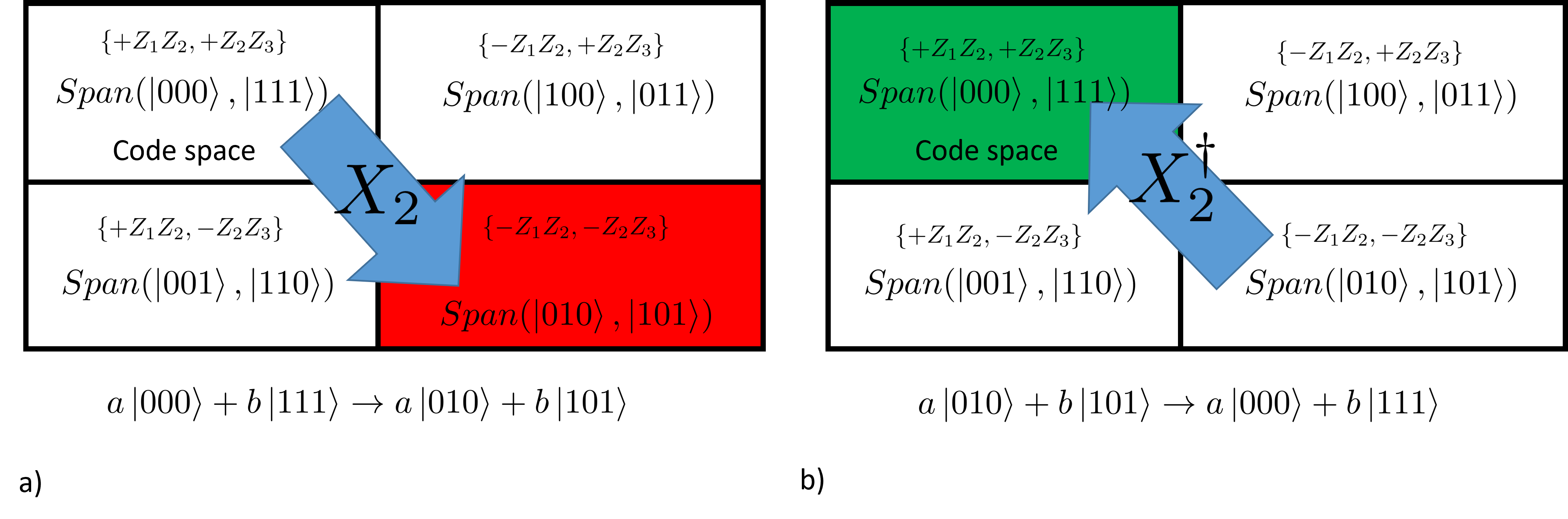
We see that the physics we are explaining here is analog to what we presented in 3.1. But it is phrased in the language of stabilizer codes, which, as we are going to see, allows to describe the physics in much simpler terms.

We can also wonder what happens if two errors are affecting the qubits, which is more than what the code is designed to protect. This is represented on the figure 3.3.

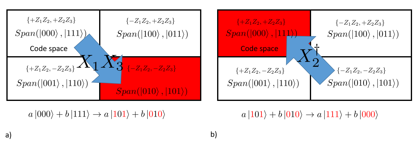
We see that the correction is then made in a wrong manner, and the state of the system might be back in the code space, but the logical qubit has now what is called a logical error: initially, we had a logical qubit being $a\left|{0_{L}}\right\rangle+b\left|{1_{L}}\right\rangle$ , and after the error and correction, it became $a\left|{1_{L}}\right\rangle+b\left|{0_{L}}\right\rangle$ . If the logical qubit was used in a computation, the outcome of the computation might then be wrong. Once a logical error occurs, it is in principle not possible to recover the initial data (excepted if, by some luck, a subsequent logical error will compensate this one).

The example of the three-qubit code is very instructive as it contains the main logic behind the stabilizer codes. For this reason, we are now ready to introduce Steane code which is able to correct for an arbitrary single-qubit error occurring on any physical qubit composing the logical one.

3.3 Correcting arbitrary single qubit errors with Steane stabilizer code

The Steane code is a stabilizer code that is able to protect a quantum state from an arbitrary single-qubit error. To be able to do it, it uses $7$ physical qubits that are encoding one logical qubit.

3.3.1 The stabilizers of Steane code

The code space of the Steane code¹¹¹¹ 11 Actually, the definition of a code is the same as the definition of code space, the two terms are synonym: thus Steane code is actually by definition the space that is stabilized by the stabilizers provided in (3.15). is the space of dimension $k=1$ that is contained in the space of dimension $n=7$ stabilized by the $6$ following $7$ -Pauli operators. We call those operators the stabilizers of Steane code.

		$\displaystyle g_{1}=X_{4}X_{5}X_{6}X_{7}$
		$\displaystyle g_{2}=X_{2}X_{3}X_{6}X_{7}$
		$\displaystyle g_{3}=X_{1}X_{3}X_{5}X_{7}$
		$\displaystyle g_{4}=Z_{4}Z_{5}Z_{6}Z_{7}$
		$\displaystyle g_{5}=Z_{2}Z_{3}Z_{6}Z_{7}$
		$\displaystyle g_{6}=Z_{1}Z_{3}Z_{5}Z_{7}$		(3.15)

We recall that to be ”stabilized” by operators means to be in the common eigenspace of eigenvalue $+1$ of those operators. This is not entirely obvious to see it here, but by performing appropriate calculations, we could show that this list of stabilizers satisfy the conditions we gave in the last paragraph of the section 3.2.1. First, they all commute together. Then, any product involving those stabilizers cannot be equal to $-I$ . Those two conditions ensure that the stabilized space is not reduced to $\{0\}$ . They also form an independent family: any stabilizer cannot be written as a product of the others. Those conditions will imply that each of the stabilizers participates in stabilizing a smaller subspace: each one of them ”divides” the dimension of the Hilbert space by two. The total Hilbert space being of dimension $2^{7}$ , we end up with a code space being of dimension $2^{7}/2^{6}=2$ : a unique logical qubit is being protected. Rigorous derivations behind our claims can be found in [66].

3.3.2 Defining the logical states

At this point, the code space is well defined. We saw that $7$ physical qubits are encoding one logical qubit, and this logical qubit lives by definition in the two-dimensional code space. But we would like to know what is now playing the role of the $\left|{0}\right\rangle$ and $\left|{1}\right\rangle$ states in the computation which we write $\left|{0_{L}}\right\rangle$ and $\left|{1_{L}}\right\rangle$ to recall that they are logical qubit states. In principle, any two orthogonal states of the code space could play this role. One possible way to define them is also based on the stabilizer formalism. For this, we can notice that for a qubit, $\left|{0}\right\rangle$ can be defined as the state stabilized by $Z$ (and $\left|{1}\right\rangle$ by the state stabilized by $-Z$ ). Adopting the same philosophy, we can first define the logical $Z$ operators, $Z_{L}$ in order to, then, define the states $\left|{0_{L}}\right\rangle$ and $\left|{1_{L}}\right\rangle$ . Defining $Z_{L}$ actually follows the same logic as what we would need to define the code space: we want to build $Z_{L}$ in order that $Z_{L}$ added to the list of stabilizers in (3.15) stabilizes a unique¹²¹² 12 Unique up to some arbitrary global phase. state. If the properties given in the last paragraph of 3.2.1 are satisfied for the resulting list, then the state will necessarily be in the code space. The stabilized state will by definition be $\left|{0_{L}}\right\rangle$ . We can also define $\left|{1_{L}}\right\rangle$ as the state stabilized by the same list, up to the modification $Z_{L}\to-Z_{L}$ . One possible choice is to consider¹³¹³ 13 It would satisfy the conditions given in the last paragraph of 3.2.1.:

\displaystyle Z_{L}\equiv Z_{1}Z_{2}Z_{3}Z_{4}Z_{5}Z_{6}Z_{7}

(3.16)

From it (and the expression of the stabilizers), we can write down the expression of the logical states, a proper calculation [66] would show that:

		$\displaystyle\left\|{0_{L}}\right\rangle=\frac{1}{\sqrt{8}}\left(\left\|{0000000}\right\rangle+\left\|{0001111}\right\rangle+\left\|{0110011}\right\rangle+\left\|{0111100}\right\rangle+\left\|{1010101}\right\rangle+\left\|{1011010}\right\rangle+\left\|{1100110}\right\rangle+\left\|{1101001}\right\rangle\right)$		(3.17)
		$\displaystyle\left\|{1_{L}}\right\rangle=\frac{1}{\sqrt{8}}\left(\left\|{1111111}\right\rangle+\left\|{0101010}\right\rangle+\left\|{1001100}\right\rangle+\left\|{0011001}\right\rangle+\left\|{1110000}\right\rangle+\left\|{0100101}\right\rangle+\left\|{1000011}\right\rangle+\left\|{0010110}\right\rangle\right)$		(3.18)

As we see, their expression is rather cumbersome. This is also why the stabilizer formalism is used; it allows to be very economical in order to describe the quantum states. The interest in having written them is that we see that those states are really ”not obvious”: they are highly entangled states. But this is not a coincidence. This code is able to protect against local errors (because it can correct errors occurring on a single physical qubit). To do it, it will encode the information in a delocalized way, thus using highly entangled states.

Now that a computational basis for the logical state has been defined, an important question remains: how to manipulate this logical qubit? For any given unitary that the algorithm requires, how can we ”translate” it to the logical qubit level? The answer to this question can easily be accessed by noticing that (i) the Pauli matrices $\{I,X,Y,Z\}$ form a basis for the operators acting on a qubit, (ii) $Y=iZX$ . Indeed, if we are able to define the logical $X$ operator: $X_{L}$ , then any single logical qubit operation could be described using $X_{L}$ and $Z_{L}$ . For this, we can build $X_{L}$ in such a way that it satisfies all the properties given in the last paragraph of the section 3.2.1 (to make sure that $X_{L}$ added on the stabilizer list will stabilize a unique quantum state), and that it anti-commutes with $Z_{L}$ in order to properly respect the Pauli algebra. An operator satisfying those conditions is:

\displaystyle X_{L}\equiv X_{1}X_{2}X_{3}X_{4}X_{5}X_{6}X_{7}

(3.19)

And now that single logical qubit Pauli operators are defined, by using the tensor product, we can define multi logical qubit Pauli operators, and we can finally build an arbitrary operator. Thus, conceptually, we know how to manipulate the logical state. But in practice, the situation is more complicated. Indeed what we need is to implement operations in a robust manner such that we do not introduce ”too many” errors when manipulating the qubit. This is the topic of fault tolerance that we introduce in the next pages.

3.3.3 Error detection and correction

Now that Steane code has been described and that we understand how the logical computational states are defined, we need to understand how errors are detected and corrected. First, we recall that Steane code is able to correct for an arbitrary¹⁴¹⁴ 14 As it is able to correct for $X$ and $Z$ errors, it is able to correct for an arbitrary single-qubit error from the theorem (3.1.3). single-qubit error affecting one physical qubit composing the logical qubit. Typically, if two physical qubits composing the logical one are affected by an error at the same time, it will not be possible to recover from it¹⁵¹⁵ 15 This is not entirely true: Steane code cannot correct for errors such as $X_{1}X_{2}$ but it can correct for error like $X_{1}Z_{2}$ for instance. Typically if two different errors are affecting two different qubits, the recovery will succeed.. The code is first doing the detection of the error followed by the correction. We describe those two steps here.

3.3.3.1 Error detection: the syndrome measurement

Here, we are going to explain with a little bit more details the principle of error detection, also called syndrome measurement. The principle is very similar to the measurement of the stabilizers we presented for the three-qubit code in section 3.2.2, but in order to properly understand the correction procedure and the principle of error discretization, we consider an arbitrary error channel and explain how this correction works in practice. We will also see that even if no correction is being applied, the simple fact to detect the error already introduces a ”partial” correction.

We consider an error channel $\mathcal{E}$ described by a family of Kraus operators $\{M_{k}\}$ . This error channel is affecting the state of the physical qubits encoding the logical qubit: $\left|{\psi_{A}}\right\rangle$ . Considering in the description the environment with which $\left|{\psi_{A}}\right\rangle$ will get entangled (it is a way to model the effect of the noise as we explained in the text around (3.3)), we can describe the state of the system+environment once the noise has acted as $\left|{\Psi}\right\rangle=\sum_{k}M_{k}\left|{\psi_{A}}\right\rangle\left|{b_{k}}\right\rangle$ (the family of orthogonal states $\{\left|{b_{k}}\right\rangle\}$ are associated to the environment). Now, we can decompose the Kraus operators on some $n$ -Pauli operators $\{E_{i}\}$ such that: $M_{k}=\sum_{i}c_{ik}E_{i}$ for some complex coefficients $c_{ik}$ . This is always possible as the $n$ -Pauli operator form a basis on which any operator acting on $n$ qubits can be decomposed [66]. If we define $\left|{\widetilde{b}_{i}}\right\rangle=\sum_{k}c_{ik}\left|{b_{k}}\right\rangle$ , we obtain:

\displaystyle\left|{\Psi}\right\rangle=\sum_{i}E_{i}\left|{\psi_{A}}\right\rangle\left|{\widetilde{b}_{i}}\right\rangle

(3.20)

At this point, we can clarify what it means to have only single physical qubit errors. It means that any of the $n$ -Pauli operators $E_{i}$ actually contains one non-trivial Pauli operator. For instance, it would mean that it is allowed to have $E_{i}=X_{3}$ but not $E_{i}=Z_{1}Z_{2}$ as the latter contains Pauli operators affecting two different qubits. We can also see here that the notion of having or not having an error is less clear than with the Kraus decomposition: as the different states $\{\left|{\widetilde{b}_{i}}\right\rangle\}$ do not represent an orthonormal family, having an error $E_{i}$ is not entirely distinguishable from having an error $E_{j}$ for instance.

Now, in order to detect the error, we have to measure all the stabilizers on the state $\left|{\Psi}\right\rangle$ in (3.20). In a similar fashion as what was done in the section 3.2.2, we will make use of the that fact $E_{i}$ commutes or anti-commutes with any of the stabilizer $g_{k}$ of Steane code. If it commutes with it, $g_{k}$ will still stabilize the state. Otherwise, $-g_{k}$ will. For this reason, any term $E_{i}\left|{\psi_{A}}\right\rangle$ in the sum (3.20) will, after measurement, bring the state in a subspace that will be stabilized by $\pm g_{k}$ for any stabilizer $g_{k}$ given in (3.15). By measuring the eigenvalues of the Stabilizers, the experimentalist will then be able to deduce which error occurred and will be able to correct it. We also notice that the syndrome measurement already performs a ”partial” correction. Indeed, because a projective measurement is performed, once the syndrome measurement is being performed, any overlap of the system between different eigenspaces of the stabilizers will be destroyed. If we think about the example of the three-qubit code, the state of the system after syndrome measurement would either be in one of the four rectangles of the figure 3.2, but it cannot extend on different rectangles at the same time. We are going to see in the section 3.4 that this syndrome measurement will then be ”enough” in practice if classical processing is keeping in memory the outcome result: the syndrome does the ”most important” part of the correction.

Now we simplified a bit the story by saying that from the measurement outcome of the stabilizers, we can directly identify which error occured¹⁶¹⁶ 16 For the conditions on the errors given in this paragraph, different errors can in principle lead to the same syndrome while ensuring a correction to be possible.. We saw with the three-qubit code example that if we allowed for two physical qubit errors such as $X_{1}X_{3}$ it is not possible to identify that it is the error that occurred. The conditions we need to allow the different errors to be corrected is that for all $(i,j)$ : $E_{i}E_{j}^{\dagger}$ is either a product of the stabilizers, either anti-commutes with at least one of the stabilizers [66]. For Steane code, if we assume that all the possible n-Pauli errors $\{E_{i}\}$ actually contain only one non-trivial Pauli operator, we can check that those conditions will be satisfied (we provided those conditions for the sake of completeness).

3.3.3.2 Error correction:

The error correction procedure is very simple; once the syndrome has been found, the experimentalist will find which error occurred, and it simply has to apply its inverse. For instance if an error $X_{1}$ occurred, the stabilizer of the state containing the error will be $\{g_{1},g_{2},g_{3},g_{4},g_{5},-g_{6}\}$ . The fact that the last stabilizer changed allows the experimentalist to deduce that the error $X_{1}$ occurred, and it will then apply $X_{1}$ on the system to implement the correction (of course, it works if no more than one error occurred).

3.4 Fault-tolerant quantum computing

3.4.1 Error correction is not enough: the need for fault-tolerance

In the previous section, we explained how the Steane code is constructed, and we gave the basic intuition behind the more general formalism of Stabilizer codes. We showed that it is conceptually possible to detect and correct errors occurring on quantum systems. But unfortunately, this is not enough in practice. Indeed, so far, we assumed that we had a given quantum state on which we want the information to be preserved, and that after the noise is occurring, we can perfectly detect and correct for the errors it induced. This is, of course, an unrealistic assumption: those operations will be noisy as well. Fault-tolerant quantum computing is the step further. It explains how it is possible to implement successfully quantum error correction, acknowledging that this is also a noisy operation by providing explicit circuit construction. Those circuits will be at the roots of the energetic estimations we will do in the next chapters. It will also provide us with all the theoretical tools required to understand how to scale up the level of protection: we will see that given some conditions, the effective noise felt by the logical qubits can be put as close to zero as desired.

To understand the issue with the sole use of error correction, let us design a simple circuit that allows measuring all the stabilizers of the Steane code. In order to do so, we will need the following property that allows us to measure observables easily. Its proof is given in the appendix.

Property 3.4.1.

Measuring observable having $\pm 1$ as eigenvalues

To measure an observable $M$ (possibly acting on multiple qubits) that admits eigenvalues $\pm 1$ , one can design the following circuit.

	$\displaystyle(\widehat{a}+\widehat{a}^{\dagger})^{2}\left\|{n}\right\rangle$	$\displaystyle=(\widehat{a}+\widehat{a}^{\dagger})\left(\sqrt{n}\left\|{n-1}\right\rangle+\sqrt{n+1}\left\|{n+1}\right\rangle\right)$
		$\displaystyle=\left(\sqrt{n(n-1)}\left\|{n-2}\right\rangle+(2n+1)\left\|{n}\right\rangle+\sqrt{(n+1)(n+2)}\left\|{n+2}\right\rangle\right)$		(B.1)

		$\displaystyle p_{L}^{(k)}=\eta_{\text{thr}}\left(\frac{\eta}{\eta_{\text{thr}}}\right)^{2^{k}}$		(3.29)
		$\displaystyle\eta_{\text{thr}}\equiv\frac{1}{\binom{A}{2}}$		(3.30)

		$\displaystyle N_{L}^{*}=O(N_{L}(\log(N_{L}))^{\log_{2}(l)})$		(3.35)
		$\displaystyle D_{L}^{*}=O(D_{L}(\log(N_{L}))^{\log_{2}(d)}),$		(3.36)

	lvl-0 cNOT	lvl-0 Single	lvl-0 Identity	lvl-0 Measurement
lvl-1 cNOT	$135$	$56$	$72$	$56$
lvl-1 Single	$64$	$35$	$36$	$28$
lvl-1 Identity	$64$	$28$	$43$	$28$
lvl-1 Measurement	$0$	$0$	$0$	$7$

$\displaystyle(\mathcal{R}\circ\mathcal{E})(P_{C}\rho P_{C})$	$\displaystyle=\sum_{i,j}U_{j}^{\dagger}P_{j}M_{i}P_{C}\rho P_{C}M_{i}^{\dagger}P_{j}U_{j}$
	$\displaystyle=\sum_{i,j}c_{ii}U_{j}^{\dagger}P_{j}P_{i}U_{i}\rho U_{i}^{\dagger}P_{i}^{\dagger}P_{j}U_{j}$
	$\displaystyle=\sum_{i}c_{ii}U_{i}^{\dagger}P_{i}U_{i}\rho U_{i}^{\dagger}P_{i}U_{i}$
	$\displaystyle=\left(\sum_{i}c_{ii}\right)P_{C}\rho P_{C}=P_{C}\rho P_{C}$	(A.4)

		$\displaystyle\widetilde{F}_{n}=\sum_{j}u_{jn}M_{j}$
		$\displaystyle c_{mm}=d_{mm}$		(A.7)

Gate	Input Pauli error $E$	Output error $A_{E}$
cNOT	$X_{1}$	$X_{1}X_{2}$
	$X_{2}$	$X_{2}$
	$Z_{1}$	$Z_{1}$
	$Z_{2}$	$Z_{1}Z_{2}$
H	$X$	$Z$
H	$Z$	$X$
X	$X$	$X$
X	$Z$	$-Z$
Y	$X$	$-X$
Y	$Z$	$-Z$
Z	$X$	$-X$
Z	$Z$	$Z$

		$\displaystyle\eta(k)=\eta_{0}f(k)$		(4.6)
		$\displaystyle\eta_{0}=\alpha R_{L}^{-\beta}$		(4.7)
		$\displaystyle f(k)=N(k)^{\beta}=D^{\beta k}$		(4.8)

		$\displaystyle k_{\max}=\bigg\lceil\widetilde{k}\bigg\rceil-1$		(4.10)
		$\displaystyle\widetilde{k}=-\frac{\ln(\eta_{0}D^{\beta}/\eta_{\text{thr}})}{\ln(D^{\beta})}$		(4.11)

		$\displaystyle\Delta_{z,d=1}(N_{\text{qubits}})=\frac{2\delta}{a^{z}}\sum_{j>0}^{N_{\text{qubits}}/2}\frac{1}{j^{z}}$		(4.18)
		$\displaystyle\Delta_{z,d=2}(N_{\text{qubits}})=\frac{\delta}{a^{z}}\sum^{\sqrt{N_{\text{qubits}}}/2}_{i=-\sqrt{N_{\text{qubits}}}/2}\sum_{j=-\sqrt{N(k)}/2}^{\sqrt{N_{\text{qubits}}}/2}\frac{c_{ij}}{\sqrt{i^{2}+j^{2}}^{z}},$		(4.19)

		$\displaystyle\Delta^{(0)}_{z<d,d=1}=\frac{\delta Q_{L}^{1-z}2^{z}}{a^{z}(1-z)}$		(4.21)
		$\displaystyle\Delta^{(0)}_{z<d,d=2}=\frac{\delta 2^{z}C_{z}Q_{L}^{1-z/2}}{a^{z}}$		(4.22)

		$\displaystyle\int_{n}^{n+1}dx\frac{1}{x^{z}}\leq\frac{1}{n^{z}}\leq\int_{n-1}^{n}dx\frac{1}{x^{z}}$		(B.3)
		$\displaystyle\int_{2}^{M+1}dx\frac{1}{x^{z}}\leq\sum_{n=2}^{M}\frac{1}{n^{z}}\leq\int_{1}^{M}dx\frac{1}{x^{z}}$		(B.4)

		$\displaystyle\eta(k,d=1,z<1)\sim\eta_{0}(1,z<1)D^{\beta_{z}k}$		(B.8)
		$\displaystyle\eta_{0}(1,z<1)=e^{1+1/2e}2\sqrt{\frac{\delta t_{0}Q_{L}^{1-z}}{a^{z}(1-z)2^{1-z}}}$		(B.9)
		$\displaystyle\beta=\frac{1-z}{2}$		(B.10)

		$\displaystyle\Delta_{z,d=2}(k)=\frac{4\delta}{a^{z}}\left(\widetilde{\Delta}_{II,z}+\widetilde{\Delta}_{I,z}\right)$		(B.12)
		$\displaystyle\widetilde{\Delta}_{II,z}=\sum_{n=1}^{M}\sum_{m=1}^{M}\frac{1}{(m^{2}+n^{2})^{z/2}}$		(B.13)
		$\displaystyle\widetilde{\Delta}_{I,z}=\sum_{m=1}^{M}\frac{1}{m^{z}},$		(B.14)

	$\displaystyle I_{a,z}(M)=$	$\displaystyle\int_{\arctan(a/M)}^{\pi/4}d\theta\int_{a/\sin(\theta)}^{M/\cos(\theta)}dr\ r^{1-z}+\int_{\pi/4}^{\arctan(M/a)}d\theta\int_{a/\cos(\theta)}^{M/\sin(\theta)}dr\ r^{1-z}$
		$\displaystyle=M^{2-z}\frac{2}{2-z}\int_{\pi/4}^{\arctan(M/a)}d\theta\frac{1}{\sin(\theta)^{2-z}}-2\frac{a^{2-z}}{2-z}\int_{\arctan(a/M)}^{\pi/4}d\theta\frac{1}{\sin(\theta)^{2-z}}$		(B.17)

		$\displaystyle I_{a}(M)\sim M^{2-z}C_{z}$		(B.21)
		$\displaystyle C_{z}=\frac{2}{2-z}\int_{\pi/4}^{\pi/2}d\theta\frac{1}{\sin(\theta)^{2-z}}.$		(B.22)

		$\displaystyle\Delta_{z<d,d=2}(k)\sim\frac{2^{z}\delta Q_{L}^{1-z/2}}{a^{z}}C_{z}D^{k(1-z/2)}$		(B.23)
		$\displaystyle\eta=e^{1+1/2e}\sqrt{2\Delta(k)t_{0}}\sim e^{1+1/2e}\sqrt{2t_{0}\frac{2^{z}\delta Q_{L}^{1-z/2}}{a^{z}}C_{z}}D^{k(1/2-z/4)}$		(B.24)

		$\displaystyle\partial_{\delta_{j}}P(\bm{\delta})<0$		(3.3)
		$\displaystyle\partial_{\delta_{j}}\mathcal{M}(\bm{\delta})>0$		(3.4)

		$\displaystyle a=0$		(3.21)
		$\displaystyle b^{\text{cNOT}}=\frac{300-T_{\text{Q}}}{T_{\text{Q}}}AP_{g}$		(3.22)
		$\displaystyle b^{\text{Id}}=0,$		(3.23)

		$\displaystyle N_{\text{during }\tau_{L}}^{\text{cNOT}}(k)=\frac{1}{3}199^{k}(2\overline{N}_{L,\parallel}^{\text{cNOT}}+\overline{N}_{L,\parallel}^{\text{Id}}+\overline{N}_{L,\parallel}^{\text{1qb}})+\frac{7^{k}}{3}\left(\overline{N}_{L,\parallel}^{\text{cNOT}}-\overline{N}_{L,\parallel}^{\text{Id}}-\overline{N}_{L,\parallel}^{\text{1qb}}\right)$		(3.32)
		$\displaystyle N_{\text{during }\tau_{L}}^{\text{1qb}}(k)=\frac{7}{48}199^{k}(2\overline{N}_{L,\parallel}^{\text{cNOT}}+\overline{N}_{L,\parallel}^{\text{Id}}+\overline{N}_{L,\parallel}^{\text{1qb}})+\frac{7^{k}}{48}\left(-14\overline{N}_{L,\parallel}^{\text{cNOT}}-7\overline{N}_{L,\parallel}^{\text{Id}}+41\ \overline{N}_{L,\parallel}^{\text{1qb}}\right)$		(3.33)
		$\displaystyle N_{\text{during }\tau_{L}}^{\text{Id}}(k)=\frac{3}{16}199^{k}(2\overline{N}_{L,\parallel}^{\text{cNOT}}+\overline{N}_{L,\parallel}^{\text{Id}}+\overline{N}_{L,\parallel}^{\text{1qb}})+\frac{7^{k}}{16}\left(-6\overline{N}_{L,\parallel}^{\text{cNOT}}+13\overline{N}_{L,\parallel}^{\text{Id}}-3\overline{N}_{L,\parallel}^{\text{1qb}}\right)$		(3.34)
		$\displaystyle N_{\text{during }\tau_{L}}^{\text{Meas}}(k)=\frac{7}{48}199^{k}(2\overline{N}_{L,\parallel}^{\text{cNOT}}+\overline{N}_{L,\parallel}^{\text{Id}}+\overline{N}_{L,\parallel}^{\text{1qb}})+\frac{7^{k}}{48}\left(-14\overline{N}_{L,\parallel}^{\text{cNOT}}-7\overline{N}_{L,\parallel}^{\text{Id}}+48\overline{N}_{L,\parallel}^{\text{Meas}}-7\overline{N}_{L,\parallel}^{\text{1qb}}\right)$		(3.35)

		$\displaystyle\overline{N}_{P,\parallel}^{\text{cNOT}}(k)\approx\frac{1}{3}\left(\frac{199}{3}\right)^{k}(2\overline{N}_{L,\parallel}^{\text{cNOT}}+\overline{N}_{L,\parallel}^{\text{Id}}+\overline{N}_{L,\parallel}^{\text{1qb}})$		(3.36)
		$\displaystyle\overline{N}_{P,\parallel}^{\text{1qb}}(k)\approx\frac{7}{48}\left(\frac{199}{3}\right)^{k}(2\overline{N}_{L,\parallel}^{\text{cNOT}}+\overline{N}_{L,\parallel}^{\text{Id}}+\overline{N}_{L,\parallel}^{\text{1qb}})$		(3.37)
		$\displaystyle\overline{N}_{P,\parallel}^{\text{Meas}}(k)\approx\frac{7}{48}\left(\frac{199}{3}\right)^{k}(2\overline{N}_{L,\parallel}^{\text{cNOT}}+\overline{N}_{L,\parallel}^{\text{Id}}+\overline{N}_{L,\parallel}^{\text{1qb}})$		(3.38)

References

- [1] I. Fuentes-Schuller and R. B. Mann, “Alice falls into a black hole: entanglement in noninertial frames,” Physical review letters, vol. 95, no. 12, p. 120404, 2005.
- [2] J. P. Dowling and G. J. Milburn, “Quantum technology: the second quantum revolution,” Philosophical Transactions of the Royal Society of London. Series A: Mathematical, Physical and Engineering Sciences, vol. 361, no. 1809, pp. 1655–1674, 2003.
- [3] L. Jaeger, “The second quantum revolution,” Switzerland: Springer, 2018.
- [4] A. Rauschenbeutel, G. Nogues, S. Osnaghi, P. Bertet, M. Brune, J.-M. Raimond, and S. Haroche, “Coherent operation of a tunable quantum phase gate in cavity qed,” Physical Review Letters, vol. 83, no. 24, p. 5166, 1999.
- [5] Y. Nakamura, Y. A. Pashkin, and J. S. Tsai, “Rabi oscillations in a josephson-junction charge two-level system,” Physical Review Letters, vol. 87, no. 24, p. 246601, 2001.
- [6] S. Haroche and J.-M. Raimond, Exploring the quantum: atoms, cavities, and photons. Oxford university press, 2006.
- [7] C. L. Degen, F. Reinhard, and P. Cappellaro, “Quantum sensing,” Reviews of modern physics, vol. 89, no. 3, p. 035002, 2017.
- [8] S. Pirandola, B. R. Bardhan, T. Gehring, C. Weedbrook, and S. Lloyd, “Advances in photonic quantum sensing,” Nature Photonics, vol. 12, no. 12, pp. 724–733, 2018.
- [9] S. Pirandola, U. L. Andersen, L. Banchi, M. Berta, D. Bunandar, R. Colbeck, D. Englund, T. Gehring, C. Lupo, C. Ottaviani, et al., “Advances in quantum cryptography,” Advances in Optics and Photonics, vol. 12, no. 4, pp. 1012–1236, 2020.
- [10] A. Shenoy-Hejamadi, A. Pathak, and S. Radhakrishna, “Quantum cryptography: key distribution and beyond,” Quanta, vol. 6, no. 1, pp. 1–47, 2017.
- [11] J. Chen, “Review on quantum communication and quantum computation,” in Journal of Physics: Conference Series, vol. 1865, p. 022008, IOP Publishing, 2021.
- [12] N. Gisin and R. Thew, “Quantum communication,” Nature photonics, vol. 1, no. 3, pp. 165–171, 2007.
- [13] L. Moerel and P. Timmers, “Reflections on digital sovereignty,” EU Cyber Direct, Research in Focus series, 2021.
- [14] D. J. Bernstein and T. Lange, “Post-quantum cryptography,” Nature, vol. 549, no. 7671, pp. 188–194, 2017.
- [15] C. Gidney and M. Ekerå, “How to factor 2048 bit rsa integers in 8 hours using 20 million noisy qubits,” Quantum, vol. 5, p. 433, 2021.
- [16] F. Arute, K. Arya, R. Babbush, D. Bacon, J. C. Bardin, R. Barends, R. Biswas, S. Boixo, F. G. Brandao, D. A. Buell, et al., “Quantum supremacy using a programmable superconducting processor,” Nature, vol. 574, no. 7779, pp. 505–510, 2019.
- [17] S. Tornow, W. Gehrke, and U. Helmbrecht, “Non-equilibrium dynamics of a dissipative two-site hubbard model simulated on the ibm quantum computer,” arXiv preprint arXiv:2011.11059, 2020.
- [18] D. García-Martín and G. Sierra, “Five experimental tests on the 5-qubit ibm quantum computer,” arXiv preprint arXiv:1712.05642, 2017.
- [19] Intel. https://www.intel.fr/content/www/fr/fr/research/quantum-computing.html.
- [20] M. Motta, C. Sun, A. T. Tan, M. J. O’Rourke, E. Ye, A. J. Minnich, F. G. Brandão, and G. K.-L. Chan, “Determining eigenstates and thermal states on a quantum computer using quantum imaginary time evolution,” Nature Physics, vol. 16, no. 2, pp. 205–210, 2020.
- [21] J. A. Jones and M. Mosca, “Implementation of a quantum algorithm on a nuclear magnetic resonance quantum computer,” The Journal of chemical physics, vol. 109, no. 5, pp. 1648–1653, 1998.
- [22] J. Raimond and S. Haroche, “Quantum computing: dream or nightmare,” Phys. Today, vol. 49, no. 8, pp. 51–52, 1996.
- [23] P. Aliferis, D. Gottesman, and J. Preskill, “Quantum accuracy threshold for concatenated distance-3 codes,” arXiv preprint quant-ph/0504218, 2005.
- [24] P. Aliferis, D. Gottesman, and J. Preskill, “Accuracy threshold for postselected quantum computation,” arXiv preprint quant-ph/0703264, 2007.
- [25] C. Chamberland, T. Jochym-O’Connor, and R. Laflamme, “Overhead analysis of universal concatenated quantum codes,” Physical Review A, vol. 95, no. 2, p. 022313, 2017.
- [26] M. Suchara, A. Faruque, C.-Y. Lai, G. Paz, F. T. Chong, and J. Kubiatowicz, “Comparing the overhead of topological and concatenated quantum error correction,” arXiv preprint arXiv:1312.2316, 2013.
- [27] R. Schutjens, F. A. Dagga, D. Egger, and F. Wilhelm, “Single-qubit gates in frequency-crowded transmon systems,” Physical Review A, vol. 88, no. 5, p. 052330, 2013.
- [28] L. Theis, F. Motzoi, and F. Wilhelm, “Simultaneous gates in frequency-crowded multilevel systems using fast, robust, analytic control shapes,” Physical Review A, vol. 93, no. 1, p. 012324, 2016.
- [29] D. Rosenberg, S. J. Weber, D. Conway, D.-R. W. Yost, J. Mallek, G. Calusine, R. Das, D. Kim, M. E. Schwartz, W. Woods, et al., “Solid-state qubits: 3d integration and packaging,” IEEE Microwave Magazine, vol. 21, no. 8, pp. 72–85, 2020.
- [30] C. Monroe and J. Kim, “Scaling the ion trap quantum processor,” Science, vol. 339, no. 6124, pp. 1164–1169, 2013.
- [31] C. D. Bruzewicz, J. Chiaverini, R. McConnell, and J. M. Sage, “Trapped-ion quantum computing: Progress and challenges,” Applied Physics Reviews, vol. 6, no. 2, p. 021314, 2019.
- [32] P. Wang, C.-Y. Luan, M. Qiao, M. Um, J. Zhang, Y. Wang, X. Yuan, M. Gu, J. Zhang, and K. Kim, “Single ion qubit with estimated coherence time exceeding one hour,” Nature communications, vol. 12, no. 1, pp. 1–8, 2021.
- [33] M. Kjaergaard, M. E. Schwartz, J. Braumüller, P. Krantz, J. I.-J. Wang, S. Gustavsson, and W. D. Oliver, “Superconducting qubits: Current state of play,” Annual Review of Condensed Matter Physics, vol. 11, pp. 369–395, 2020.
- [34] R. Hanson, L. P. Kouwenhoven, J. R. Petta, S. Tarucha, and L. M. Vandersypen, “Spins in few-electron quantum dots,” Reviews of modern physics, vol. 79, no. 4, p. 1217, 2007.
- [35] P. Krantz, M. Kjaergaard, F. Yan, T. P. Orlando, S. Gustavsson, and W. D. Oliver, “A quantum engineer’s guide to superconducting qubits,” Applied Physics Reviews, vol. 6, no. 2, p. 021318, 2019.
- [36] S. Slussarenko and G. J. Pryde, “Photonic quantum information processing: A concise review,” Applied Physics Reviews, vol. 6, no. 4, p. 041303, 2019.
- [37] P. Kok, W. J. Munro, K. Nemoto, T. C. Ralph, J. P. Dowling, and G. J. Milburn, “Linear optical quantum computing with photonic qubits,” Reviews of modern physics, vol. 79, no. 1, p. 135, 2007.
- [38] B. Criger, G. Passante, D. Park, and R. Laflamme, “Recent advances in nuclear magnetic resonance quantum information processing,” Philosophical Transactions of the Royal Society A: Mathematical, Physical and Engineering Sciences, vol. 370, no. 1976, pp. 4620–4635, 2012.
- [39] R. Maurand, X. Jehl, D. Kotekar-Patil, A. Corna, H. Bohuslavskyi, R. Laviéville, L. Hutin, S. Barraud, M. Vinet, M. Sanquer, et al., “A cmos silicon spin qubit,” Nature communications, vol. 7, no. 1, pp. 1–6, 2016.
- [40] M. Vinet, L. Hutin, B. Bertrand, S. Barraud, J.-M. Hartmann, Y.-J. Kim, V. Mazzocchi, A. Amisse, H. Bohuslavskyi, L. Bourdet, et al., “Towards scalable silicon quantum computing,” in 2018 IEEE International Electron Devices Meeting (IEDM), pp. 6–5, IEEE, 2018.
- [41] J. C. Bardin, E. Jeffrey, E. Lucero, T. Huang, O. Naaman, R. Barends, T. White, M. Giustina, D. Sank, P. Roushan, et al., “29.1 a 28nm bulk-cmos 4-to-8ghz¡ 2mw cryogenic pulse modulator for scalable quantum computing,” in 2019 IEEE International Solid-State Circuits Conference-(ISSCC), pp. 456–458, IEEE, 2019.
- [42] B. Patra, J. P. Van Dijk, A. Corna, X. Xue, N. Samkharadze, A. Sammak, G. Scappucci, M. Veldhorst, L. M. Vandersypen, M. Babaie, et al., “A scalable cryo-cmos 2-to-20ghz digitally intensive controller for 4 32 frequency multiplexed spin qubits/transmons in 22nm finfet technology for quantum computers,” in 2020 IEEE International Solid-State Circuits Conference, ISSCC 2020, pp. 304–306, Institute of Electrical and Electronics Engineers (IEEE), 2020.
- [43] R. McDermott, M. Vavilov, B. Plourde, F. Wilhelm, P. Liebermann, O. Mukhanov, and T. Ohki, “Quantum–classical interface based on single flux quantum digital logic,” Quantum science and technology, vol. 3, no. 2, p. 024004, 2018.
- [44] V. K. Semenov and D. V. Averin, “Sfq control circuits for josephson junction qubits,” IEEE transactions on applied superconductivity, vol. 13, no. 2, pp. 960–965, 2003.
- [45] E. P. DeBenedictis, “Adiabatic circuits for quantum computer control,” in 2020 International Conference on Rebooting Computing (ICRC), pp. 42–49, IEEE, 2020.
- [46] A. G. Fowler, M. Mariantoni, J. M. Martinis, and A. N. Cleland, “Surface codes: Towards practical large-scale quantum computation,” Physical Review A, vol. 86, no. 3, p. 032324, 2012.
- [47] E. Dennis, A. Kitaev, A. Landahl, and J. Preskill, “Topological quantum memory,” Journal of Mathematical Physics, vol. 43, no. 9, pp. 4452–4505, 2002.
- [48] B. M. Terhal, J. Conrad, and C. Vuillot, “Towards scalable bosonic quantum error correction,” Quantum Science and Technology, vol. 5, no. 4, p. 043001, 2020.
- [49] N. Ofek, A. Petrenko, R. Heeres, P. Reinhold, Z. Leghtas, B. Vlastakis, Y. Liu, L. Frunzio, S. Girvin, L. Jiang, et al., “Extending the lifetime of a quantum bit with error correction in superconducting circuits,” Nature, vol. 536, no. 7617, pp. 441–445, 2016.
- [50] K. Noh and C. Chamberland, “Fault-tolerant bosonic quantum error correction with the surface–gottesman-kitaev-preskill code,” Physical Review A, vol. 101, no. 1, p. 012316, 2020.
- [51] D. Aharonov and M. Ben-Or, “Fault-tolerant quantum computation with constant error rate,” SIAM Journal on Computing, 2008.
- [52] U. Vool and M. Devoret, “Introduction to quantum electromagnetic circuits,” International Journal of Circuit Theory and Applications, vol. 45, no. 7, pp. 897–934, 2017.
- [53] X. Gu, A. F. Kockum, A. Miranowicz, Y.-x. Liu, and F. Nori, “Microwave photonics with superconducting quantum circuits,” Physics Reports, vol. 718, pp. 1–102, 2017.
- [54] G. Wendin and V. Shumeiko, “Superconducting quantum circuits, qubits and computing,” arXiv preprint cond-mat/0508729, 2005.
- [55] S. E. Nigg, H. Paik, B. Vlastakis, G. Kirchmair, S. Shankar, L. Frunzio, M. Devoret, R. Schoelkopf, and S. Girvin, “Black-box superconducting circuit quantization,” Physical Review Letters, vol. 108, no. 24, p. 240502, 2012.
- [56] J.-L. Basdevant, “Les principes variationnels en physique,” Vuibert, Paris, 2014.
- [57] H. Goldstein, C. Poole, and J. Safko, “Classical mechanics,” 2002.
- [58] C. Cohen-Tannoudji, B. Diu, and F. Laloë, Mécanique quantique. Hermann, EDP Sciences, 1998.
- [59] D. M. Pozar, Microwave engineering. John wiley & sons, 2011.
- [60] C. W. Gardiner and M. J. Collett, “Input and output in damped quantum systems: Quantum stochastic differential equations and the master equation,” Physical Review A, vol. 31, no. 6, p. 3761, 1985.
- [61] A. A. Clerk, M. H. Devoret, S. M. Girvin, F. ardt, and R. J. Schoelkopf, “Introduction to quantum noise, measurement, and amplification,” Reviews of Modern Physics, vol. 82, no. 2, p. 1155, 2010.
- [62] E. Wiegand, B. Rousseaux, and G. Johansson, “Semiclassical analysis of dark-state transient dynamics in waveguide circuit qed,” Physical Review A, vol. 101, no. 3, p. 033801, 2020.
- [63] B. Peropadre, J. Lindkvist, I.-C. Hoi, C. Wilson, J. J. Garcia-Ripoll, P. Delsing, and G. Johansson, “Scattering of coherent states on a single artificial atom,” New Journal of Physics, vol. 15, no. 3, p. 035009, 2013.
- [64] D. F. Walls and G. J. Milburn, Quantum optics. Springer Science & Business Media, 2007.
- [65] C. Cohen-Tannoudji, J. Dupont-Roc, and G. Grynberg, Atom-photon interactions: basic processes and applications. 1998.
- [66] M. A. Nielsen and I. Chuang, “Quantum computation and quantum information,” 2002.
- [67] N. Cottet, S. Jezouin, L. Bretheau, P. Campagne-Ibarcq, Q. Ficheux, J. Anders, A. Auffèves, R. Azouit, P. Rouchon, and B. Huard, “Observing a quantum maxwell demon at work,” Proceedings of the National Academy of Sciences, vol. 114, no. 29, pp. 7561–7564, 2017.
- [68] J. Monsel, M. Fellous-Asiani, B. Huard, and A. Auffèves, “The energetic cost of work extraction,” Physical review letters, vol. 124, no. 13, p. 130601, 2020.
- [69] A. P. Place, L. V. Rodgers, P. Mundada, B. M. Smitham, M. Fitzpatrick, Z. Leng, A. Premkumar, J. Bryon, A. Vrajitoarea, S. Sussman, et al., “New material platform for superconducting transmon qubits with coherence times exceeding 0.3 milliseconds,” Nature communications, vol. 12, no. 1, pp. 1–6, 2021.
- [70] A. Somoroff, Q. Ficheux, R. A. Mencia, H. Xiong, R. V. Kuzmin, and V. E. Manucharyan, “Millisecond coherence in a superconducting qubit,” arXiv preprint arXiv:2103.08578, 2021.
- [71] C. G. Almudever, L. Lao, X. Fu, N. Khammassi, I. Ashraf, D. Iorga, S. Varsamopoulos, C. Eichler, A. Wallraff, L. Geck, et al., “The engineering challenges in quantum computing,” in Design, Automation & Test in Europe Conference & Exhibition (DATE), 2017, pp. 836–845, IEEE, 2017.
- [72] M. Werninghaus, D. J. Egger, F. Roy, S. Machnes, F. K. Wilhelm, and S. Filipp, “Leakage reduction in fast superconducting qubit gates via optimal control,” npj Quantum Information, vol. 7, no. 1, pp. 1–6, 2021.
- [73] H.-L. Huang, D. Wu, D. Fan, and X. Zhu, “Superconducting quantum computing: a review,” Science China Information Sciences, vol. 63, no. 8, pp. 1–32, 2020.
- [74] F. Yan, P. Krantz, Y. Sung, M. Kjaergaard, D. L. Campbell, T. P. Orlando, S. Gustavsson, and W. D. Oliver, “Tunable coupling scheme for implementing high-fidelity two-qubit gates,” Physical Review Applied, vol. 10, no. 5, p. 054062, 2018.
- [75] Y. Xu, J. Chu, J. Yuan, J. Qiu, Y. Zhou, L. Zhang, X. Tan, Y. Yu, S. Liu, J. Li, et al., “High-fidelity, high-scalability two-qubit gate scheme for superconducting qubits,” Physical Review Letters, vol. 125, no. 24, p. 240503, 2020.
- [76] J. M. Chow, A. D. Córcoles, J. M. Gambetta, C. Rigetti, B. R. Johnson, J. A. Smolin, J. R. Rozen, G. A. Keefe, M. B. Rothwell, M. B. Ketchen, et al., “Simple all-microwave entangling gate for fixed-frequency superconducting qubits,” Physical review letters, vol. 107, no. 8, p. 080502, 2011.
- [77] S. Sheldon, E. Magesan, J. M. Chow, and J. M. Gambetta, “Procedure for systematically tuning up cross-talk in the cross-resonance gate,” Physical Review A, vol. 93, no. 6, p. 060302, 2016.
- [78] P. Bertet, C. Harmans, and J. Mooij, “Parametric coupling for superconducting qubits,” Physical Review B, vol. 73, no. 6, p. 064512, 2006.
- [79] D. C. McKay, S. Filipp, A. Mezzacapo, E. Magesan, J. M. Chow, and J. M. Gambetta, “Universal gate for fixed-frequency qubits via a tunable bus,” Physical Review Applied, vol. 6, no. 6, p. 064007, 2016.
- [80] M. D. Schwartz, Quantum field theory and the standard model. Cambridge University Press, 2014.
- [81] J. Preskill, “Lecture notes for physics 229: Quantum information and computation,” California Institute of Technology, vol. 16, p. 10, 1998.
- [82] C. Cohen-Tannoudji, B. Diu, and F. Laloë, Mécanique quantique-Tome 3. EDP sciences, 2021.
- [83] H.-P. Breuer, F. Petruccione, et al., The theory of open quantum systems. Oxford University Press on Demand, 2002.
- [84] A. R. Calderbank and P. W. Shor, “Good quantum error-correcting codes exist,” Physical Review A, vol. 54, no. 2, p. 1098, 1996.
- [85] A. Steane, “Multiple-particle interference and quantum error correction,” Proceedings of the Royal Society of London. Series A: Mathematical, Physical and Engineering Sciences, vol. 452, no. 1954, pp. 2551–2577, 1996.
- [86] Y.-C. Zheng, C.-Y. Lai, and T. A. Brun, “Efficient preparation of large-block-code ancilla states for fault-tolerant quantum computation,” Physical Review A, vol. 97, no. 3, p. 032331, 2018.
- [87] T. A. Brun, Y.-C. Zheng, K.-C. Hsu, J. Job, and C.-Y. Lai, “Teleportation-based fault-tolerant quantum computation in multi-qubit large block codes,” arXiv preprint arXiv:1504.03913, 2015.
- [88] D. Gottesman, Stabilizer codes and quantum error correction. California Institute of Technology, 1997.
- [89] D. Gottesman, “An introduction to quantum error correction and fault-tolerant quantum computation,” in Quantum information science and its contributions to mathematics, Proceedings of Symposia in Applied Mathematics, vol. 68, pp. 13–58, 2010.
- [90] E. Knill, R. Laflamme, and W. H. Zurek, “Resilient quantum computation: error models and thresholds,” Proceedings of the Royal Society of London. Series A: Mathematical, Physical and Engineering Sciences, vol. 454, no. 1969, pp. 365–384, 1998.
- [91] J. Preskill, “Reliable quantum computers,” Proceedings of the Royal Society of London. Series A: Mathematical, Physical and Engineering Sciences, vol. 454, no. 1969, pp. 385–410, 1998.
- [92] B. M. Terhal and G. Burkard, “Fault-tolerant quantum computation for local non-markovian noise,” Physical Review A, vol. 71, no. 1, p. 012336, 2005.
- [93] D. Aharonov, A. Kitaev, and J. Preskill, “Fault-tolerant quantum computation with long-range correlated noise,” Physical review letters, vol. 96, no. 5, p. 050504, 2006.
- [94] A. Jayashankar, M. D. H. Long, H. K. Ng, and P. Mandayam, “Achieving fault tolerance against amplitude-damping noise,” arXiv preprint arXiv:2107.05485, 2021.
- [95] S. J. Beale, J. J. Wallman, M. Gutiérrez, K. R. Brown, and R. Laflamme, “Quantum error correction decoheres noise,” Physical review letters, vol. 121, no. 19, p. 190501, 2018.
- [96] B. Eastin and E. Knill, “Restrictions on transversal encoded quantum gate sets,” Physical review letters, vol. 102, no. 11, p. 110502, 2009.
- [97] E. Knill, “Quantum computing with realistically noisy devices,” Nature, vol. 434, no. 7029, pp. 39–44, 2005.
- [98] L. Riesebos, X. Fu, S. Varsamopoulos, C. G. Almudever, and K. Bertels, “Pauli frames for quantum computer architectures,” in Proceedings of the 54th Annual Design Automation Conference 2017, pp. 1–6, 2017.
- [99] Y. Yang, Y. Mo, J. M. Renes, G. Chiribella, and M. P. Woods, “Covariant quantum error correcting codes via reference frames,” arXiv preprint arXiv:2007.09154, 2020.
- [100] A. Paetznick and B. W. Reichardt, “Universal fault-tolerant quantum computation with only transversal gates and error correction,” Physical review letters, vol. 111, no. 9, p. 090505, 2013.
- [101] C. Chamberland and K. Noh, “Very low overhead fault-tolerant magic state preparation using redundant ancilla encoding and flag qubits,” npj Quantum Information, vol. 6, no. 1, pp. 1–12, 2020.
- [102] D. Litinski, “Magic state distillation: Not as costly as you think,” Quantum, vol. 3, p. 205, 2019.
- [103] S. Bravyi and A. Kitaev, “Universal quantum computation with ideal clifford gates and noisy ancillas,” Physical Review A, vol. 71, no. 2, p. 022316, 2005.
- [104] C. Piltz, T. Sriarunothai, A. Varón, and C. Wunderlich, “A trapped-ion-based quantum byte with 10- 5 next-neighbour cross-talk,” Nature communications, vol. 5, no. 1, pp. 1–10, 2014.
- [105] I. Heinz and G. Burkard, “Crosstalk analysis for single-qubit and two-qubit gates in spin qubit arrays,” arXiv preprint arXiv:2105.10221, 2021.
- [106] D. C. McKay, S. Sheldon, J. A. Smolin, J. M. Chow, and J. M. Gambetta, “Three-qubit randomized benchmarking,” Physical review letters, vol. 122, no. 20, p. 200502, 2019.
- [107] M. Takita, A. W. Cross, A. Córcoles, J. M. Chow, and J. M. Gambetta, “Experimental demonstration of fault-tolerant state preparation with superconducting qubits,” Physical review letters, vol. 119, no. 18, p. 180501, 2017.
- [108] T. J. Proctor, A. Carignan-Dugas, K. Rudinger, E. Nielsen, R. Blume-Kohout, and K. Young, “Direct randomized benchmarking for multiqubit devices,” Physical review letters, vol. 123, no. 3, p. 030503, 2019.
- [109] S. Treil, Linear algebra done wrong. MTM, 2013.
- [110] R. Todd, “Operator norm,” Wolfram Mathworld, 2010.
- [111] M. Fellous-Asiani, J. H. Chai, R. S. Whitney, A. Auffèves, and H. K. Ng, “Limitations in quantum computing from resource constraints,” arXiv preprint arXiv:2007.01966, 2020.
- [112] T. Kim and B.-S. Choi, “Efficient decomposition methods for controlled-r n using a single ancillary qubit,” Scientific reports, vol. 8, no. 1, pp. 1–7, 2018.
- [113] P. Gokhale, Full-Stack, Cross-Layer Optimizations for Quantum Computing. PhD thesis, The University of Chicago, 2020.
- [114] P. Murali, N. M. Linke, M. Martonosi, A. J. Abhari, N. H. Nguyen, and C. H. Alderete, “Full-stack, real-system quantum computer studies: Architectural comparisons and design insights,” in 2019 ACM/IEEE 46th Annual International Symposium on Computer Architecture (ISCA), pp. 527–540, IEEE, 2019.
- [115] S. Rodrigo, S. Abadal, E. Alarcón, and C. G. Almudever, “Exploring a double full-stack communications-enabled architecture for multi-core quantum computers,” arXiv preprint arXiv:2009.08186, 2020.
- [116] M. Amy and V. Gheorghiu, “staq—a full-stack quantum processing toolkit,” Quantum Science and Technology, vol. 5, no. 3, p. 034016, 2020.
- [117] Y. Li, P. C. Humphreys, G. J. Mendoza, and S. C. Benjamin, “Resource costs for fault-tolerant linear optical quantum computing,” Physical Review X, vol. 5, no. 4, p. 041007, 2015.
- [118] I. H. Kim, E. Lee, Y.-H. Liu, S. Pallister, W. Pol, and S. Roberts, “Fault-tolerant resource estimate for quantum chemical simulations: Case study on li-ion battery electrolyte molecules,” arXiv preprint arXiv:2104.10653, 2021.
- [119] O. Di Matteo, V. Gheorghiu, and M. Mosca, “Fault-tolerant resource estimation of quantum random-access memories,” IEEE Transactions on Quantum Engineering, vol. 1, pp. 1–13, 2020.
- [120] O. Abah, R. Puebla, A. Kiely, G. De Chiara, M. Paternostro, and S. Campbell, “Energetic cost of quantum control protocols,” New Journal of Physics, vol. 21, no. 10, p. 103048, 2019.
- [121] J. Ikonen, J. Salmilehto, and M. Möttönen, “Energy-efficient quantum computing,” npj Quantum Information, vol. 3, no. 1, pp. 1–7, 2017.
- [122] S. Campbell and S. Deffner, “Trade-off between speed and cost in shortcuts to adiabaticity,” Physical review letters, vol. 118, no. 10, p. 100601, 2017.
- [123] S. Deffner, “Energetic cost of hamiltonian quantum gates,” arXiv preprint arXiv:2102.05118, 2021.
- [124] A. Robert, P. K. Barkoutsos, S. Woerner, and I. Tavernelli, “Resource-efficient quantum algorithm for protein folding,” npj Quantum Information, vol. 7, no. 1, pp. 1–5, 2021.
- [125] S. Krinner, S. Storz, P. Kurpiers, P. Magnard, J. Heinsoo, R. Keller, J. Luetolf, C. Eichler, and A. Wallraff, “Engineering cryogenic setups for 100-qubit scale superconducting circuit systems,” EPJ Quantum Technology, vol. 6, no. 1, p. 2, 2019.
- [126] R. Li, L. Petit, D. P. Franke, J. P. Dehollain, J. Helsen, M. Steudtner, N. K. Thomas, Z. R. Yoscovits, K. J. Singh, S. Wehner, et al., “A crossbar network for silicon quantum dot qubits,” Science advances, vol. 4, no. 7, p. eaar3960, 2018.
- [127] A. Gilchrist, N. K. Langford, and M. A. Nielsen, “Distance measures to compare real and ideal quantum processes,” Physical Review A, vol. 71, no. 6, p. 062310, 2005.
- [128] A. Carignan-Dugas, J. J. Wallman, and J. Emerson, “Bounding the average gate fidelity of composite channels using the unitarity,” New Journal of Physics, vol. 21, no. 5, p. 053016, 2019.
- [129] K. Bharti, A. Cervera-Lierta, T. H. Kyaw, T. Haug, S. Alperin-Lea, A. Anand, M. Degroote, H. Heimonen, J. S. Kottmann, T. Menke, et al., “Noisy intermediate-scale quantum (nisq) algorithms,” arXiv preprint arXiv:2101.08448, 2021.
- [130] A. Peruzzo, J. McClean, P. Shadbolt, M.-H. Yung, X.-Q. Zhou, P. J. Love, A. Aspuru-Guzik, and J. L. O’brien, “A variational eigenvalue solver on a photonic quantum processor,” Nature communications, vol. 5, no. 1, pp. 1–7, 2014.
- [131] L. Gentini, A. Cuccoli, S. Pirandola, P. Verrucchi, and L. Banchi, “Noise-assisted variational hybrid quantum-classical optimization,” arXiv preprint arXiv:1912.06744, 2019.
- [132] B. Villalonga, S. Boixo, B. Nelson, C. Henze, E. Rieffel, R. Biswas, and S. Mandrà, “A flexible high-performance simulator for verifying and benchmarking quantum circuits implemented on real hardware,” npj Quantum Information, vol. 5, no. 1, pp. 1–16, 2019.
- [133] A. . Bob. https://alice-bob.com/fr/.
- [134] QuTech, “Starmon-5 quantum processor.” https://www.quantum-inspire.com/backends/starmon-5/, 2020.
- [135] QuTech, “Spin-2 quantum processor.” https://www.quantum-inspire.com/backends/spin-2/.
- [136] M. Malekakhlagh, E. Magesan, and D. C. McKay, “First-principles analysis of cross-resonance gate operation,” Physical Review A, vol. 102, no. 4, p. 042605, 2020.
- [137] S. Kirchhoff, T. Keßler, P. J. Liebermann, E. Assémat, S. Machnes, F. Motzoi, and F. K. Wilhelm, “Optimized cross-resonance gate for coupled transmon systems,” Physical Review A, vol. 97, no. 4, p. 042348, 2018.
- [138] J. E. J. Johnson, Optimization of superconducting flux qubit readout using near-quantum-limited amplifiers. University of California, Berkeley, 2012.
- [139] M. D. Reed, Entanglement and quantum error correction with superconducting qubits. Yale University, 2014.
- [140] J. Weisend II, Cryostat Design. Springer, 2016.
- [141] C. Enss and S. Hunklinger, Tieftemperaturphysik. Springer-Verlag, 2011.
- [142] L. Le Guevel, G. Billiot, X. Jehl, S. De Franceschi, M. Zurita, Y. Thonnart, M. Vinet, M. Sanquer, R. Maurand, A. G. Jansen, et al., “19.2 a 110mk 295w 28nm fdsoi cmos quantum integrated circuit with a 2.8 ghz excitation and na current sensing of an on-chip double quantum dot,” in 2020 IEEE International Solid-State Circuits Conference-(ISSCC), pp. 306–308, IEEE, 2020.
- [143] J. Aumentado, “Superconducting parametric amplifiers: The state of the art in josephson parametric amplifiers,” IEEE Microwave Magazine, vol. 21, no. 8, pp. 45–59, 2020.
- [144] A. Korolev, V. Shnyrkov, and V. Shulga, “Note: Ultra-high frequency ultra-low dc power consumption hemt amplifier for quantum measurements in millikelvin temperature range,” Review of Scientific Instruments, vol. 82, no. 1, p. 016101, 2011.
- [145] V. Parma, “Cryostat design,” arXiv preprint arXiv:1501.07154, 2015.
- [146] M. J. Martin, C. Hughes, G. Moreno, E. B. Jones, D. Sickinger, S. Narumanchi, and R. Grout, “Energy use in quantum data centers: Scaling the impact of computer architecture, qubit performance, size, and thermal parameters,” arXiv preprint arXiv:2103.16726, 2021.
- [147] M. A. Green, “Helium refrigeration during the 50 years since the 1968 brookhaven summer study,” IEEE Transactions on Applied Superconductivity, vol. 29, no. 5, pp. 1–5, 2019.
- [148] “Cryogenic electronics and quantum information processing,” The international roadmap for devices and systems, 2020.
- [149] M. Wade, M. Davenport, M. D. C. Falco, P. Bhargava, J. Fini, D. Van Orden, R. Meade, E. Yeung, R. Ram, M. Popović, et al., “A bandwidth-dense, low power electronic-photonic platform and architecture for multi-tbps optical i/o,” in 2018 European Conference on Optical Communication (ECOC), pp. 1–3, IEEE, 2018.
- [150] J. F. Shackelford and W. Alexander, CRC materials science and engineering handbook. CRC press, 2000.
- [151] E. Marquardt, J. Le, and R. Radebaugh, “Cryogenic material properties database,” in Cryocoolers 11, pp. 681–687, Springer, 2002.
- [152] O. Mukhanov, A. Kirichenko, C. Howington, J. Walter, M. Hutchings, I. Vernik, D. Yohannes, K. Dodge, A. Ballard, B. Plourde, et al., “Scalable quantum computing infrastructure based on superconducting electronics,” in 2019 IEEE International Electron Devices Meeting (IEDM), pp. 31–2, IEEE, 2019.
- [153] B. Huard, “Private communication,” 2020.
- [154] R. Dassonneville, T. Ramos, V. Milchakov, L. Planat, É. Dumur, F. Foroughi, J. Puertas, S. Leger, K. Bharadwaj, J. Delaforce, et al., “Fast high-fidelity quantum nondemolition qubit readout via a nonperturbative cross-kerr coupling,” Physical Review X, vol. 10, no. 1, p. 011045, 2020.
- [155] J. Heinsoo, C. K. Andersen, A. Remm, S. Krinner, T. Walter, Y. Salathé, S. Gasparinetti, J.-C. Besse, A. Potočnik, A. Wallraff, et al., “Rapid high-fidelity multiplexed readout of superconducting qubits,” Physical Review Applied, vol. 10, no. 3, p. 034040, 2018.
- [156] M. Esposito, A. Ranadive, L. Planat, and N. Roch, “Perspective on traveling wave microwave parametric amplifiers,” arXiv preprint arXiv:2107.13033, 2021.
- [157] A. Ranadive, M. Esposito, L. Planat, E. Bonet, C. Naud, O. Buisson, W. Guichard, and N. Roch, “A reversed kerr traveling wave parametric amplifier,” arXiv preprint arXiv:2101.05815, 2021.
- [158] L. Planat, “Private communication,” 2021.
- [159] J. M. Rabaey, A. P. Chandrakasan, and B. Nikolić, Digital integrated circuits: a design perspective, vol. 7. Pearson education Upper Saddle River, NJ, 2003.
- [160] A. Bartolini, M. Cacciari, C. Cavazzoni, G. Tecchiolli, and L. Benini, “Unveiling eurora—thermal and power characterization of the most energy-efficient supercomputer in the world,” in 2014 Design, Automation & Test in Europe Conference & Exhibition (DATE), pp. 1–6, IEEE, 2014.
- [161] CERN, “Energy consumption.” https://www.lhc-closer.es/taking_a_closer_look_at_lhc/0.energy_consumption.
- [162] KEYCOM, “Semi-rigid cryogenic sus304 coaxial cable.” https://www.keycom.co.jp/eproducts/upj/upj2/page.htm.
- [163] D. B. Tuckerman, M. C. Hamilton, D. J. Reilly, R. Bai, G. A. Hernandez, J. M. Hornibrook, J. A. Sellers, and C. D. Ellis, “Flexible superconducting nb transmission lines on thin film polyimide for quantum computing applications,” Superconductor Science and Technology, vol. 29, no. 8, p. 084007, 2016.