Learning nonlinear feedforward: a Gaussian Process Approach Applied to a Printer with Friction

Let $G(q)$ denote a discrete-time, nonlinear SISO system, where $q$ is the forward-shift operator such that $q^{\tau}a(t):=a(t+\tau)$, $\tau\in\mathbb{Z}$. The closed-loop motion control architecture in Figure 1 is considered, where $r(t)$ denotes a predefined reference to be tracked at time $t\in\mathbb{Z}$, $y(t)$ is the system output, $e(t)$ is the tracking error and $\varepsilon(t)\sim\mathcal{N}(0,\sigma_{n}^{2})$ is a disturbance.
It is assumed that a stabilizing feedback controller $C(q)$ is available, as well as some prior feedforward controller $F(q)$. Perfect tracking is achieved for $F(q)=G^{-1}(q)$, since then

The goal in this paper is to obtain $\hat{F}(q)\approx G^{-1}(q)$ from data such that the 2-norm of the tracking error ($\|e\|_{2}$) is reduced. Moreover, task flexibility must be allowed.

The next section explains an additional assumption on the structure on $G^{-1}(q)$, before the problem formulation is formalized in Section II-C.

In order to find a feedforward controller $\hat{F}(q)\approx G^{-1}(q)$, we first impose some structure on $G^{-1}(q)$. First, note that linear sampled systems $P(z)$ of continuous-time systems $P(s)$ often contain zeros outside the unit disc, depending on the sample time and the relative degree of $P(s)$, see [1]. Consequently, $P^{-1}(z)$ may contain poles outside the unit disc. Whereas systems with poles outside the unit disc are typically viewed as causal and unstable, they may also be viewed as noncausal and stable.

In the absence of infinite preview or history, a non-causal FIR system parametrization may be used as a finite-dimensional approximation of (2):

with $\mathbf{r}_{t}:=\left[r\left(t+n_{ac}\right),\ldots,r\left(t-n_{c}\right)\right]^{\top}\in\mathcal{Y}$, where $\mathcal{Y}\subset\mathbb{R}^{n_{\theta}}$ is compact with $n_{\theta}=n_{c}+n_{ac}+1$, for reasons described in Section III-B.

In this paper, this idea is extended to nonlinear systems by assuming that the nonlinear system $G^{-1}(q)$ can be represented with a non-causal nonlinear finite impulse response (NFIR) parametrization, such that the control effort $u(t)$ required to realize output sequence $\mathbf{y}_{t}:=\left[y\left(t+n_{ac}\right),\ldots,y\left(t-n_{c}\right)\right]^{\top}\in\mathcal{Y}$ can be written as

where $f:\mathcal{Y}\rightarrow\mathbb{R}$ is an alternative form of $G^{-1}(q):\mathbb{R}\rightarrow\mathbb{R}$, in which $q$ has been eliminated.

In this paper, the aim is to model the function $f$ in (4) describing $G^{-1}$ from a dataset $\mathcal{D}=\{u(t),y(t)\}_{t=1}^{M}$, such that $f(\mathbf{r}_{t})$ yields the control effort (or feedforward signal) $u(t)$ that realizes reference sequence $\mathbf{r}_{t}:=\left[r\left(t+n_{ac}\right),\ldots,r\left(t-n_{c}\right)\right]^{\top}\in\mathcal{Y}$. Note that by learning $f$, feedforward samples $u(t)$ can be computed for any $\mathbf{r}_{t}$, i.e., task flexibility is allowed.

Next, $f$ in (4) is regarded as a Gaussian Process (GP), to learn it from data.

Hence, if $f(\mathbf{y}_{t})$ is a GP, then there exists a joint distribution between observations of $u(t)=f(\mathbf{y}_{t})+\varepsilon(t)$ and unknown feedforward samples $u(t)=f(\mathbf{r}_{t})$. It is shown next how GPs can be employed to make predictions of these feedforward samples, based on observations of $u$ and $y$.

Let the covariance between any two control effort values required for output sequences $\mathbf{y}_{t}$ be defined by a kernel function

This kernel function imposes properties such as smoothness or periodicity on $f$, as explained in detail in Section III-C. Given a dataset $\mathcal{D}=\left\{Y,\mathbf{u}\right\}$, with

and assuming a zero-mean prior on $f$, we can define the joint distribution

where $R=\left[\mathbf{r}_{1},\ldots,\mathbf{r}_{N}\right]^{\top}$ is a toeplitz matrix constructed from $r\in\mathbb{R}^{N}$, with $\mathbf{r}_{t}:=\left[r\left(t+n_{ac}\right),\ldots,r\left(t-n_{c}\right)\right]^{\top}$. The covariance matrices $K$ in (7) are constructed by evaluating $k$ for each element.

To compute the feedforward signal $\mathbf{f}(R)$ for reference $R$, the joint distribution in (7) is conditioned on the observations using Bayes’ rule. The resulting posterior distribution $p(\mathbf{f}(R)\mid Y,\mathbf{u},R)$ is a Gaussian with mean and variance

This yields an analytic expression for the expected feedforward signal required for reference $r$, as well as explicit uncertainty bounds on the feedforward signal.

Whether the realization $\mathbb{E}[\mathbf{f}(R)]$ is representative of the real function $f$ is dependent on the choice of $k$ in (5). This can be seen easily by rewriting the posterior mean (8) in scalar form as

with $\boldsymbol{\alpha}=(K(Y,Y)+\sigma_{n}^{2}I)^{-1}\mathbf{u}$. Naturally, if $k$ were to be chosen inappropriately, e.g., linear in $\mathbf{r}_{t}$, as done for linear systems in [3], no nonlinear function $f$ could be represented by the posterior mean. A particularly widely applicable type of kernel is the universal kernel.

Hence, universal kernels are structurally capable of representing any continuous $f$ through (9), even if the nonlinear structure of $f$, or equivalently, the non-causal NFIR system $G^{-1}(q)$, is unknown.

In practice, some information on $f$ may be available, such as smoothness or periodicity. This information can be exploited through stationary kernel functions, as explained in more detail in the next section.

This choice of kernel leads to a data-dependent model (9) in which control effort values $u(t)=f(\mathbf{r}_{t})$ are inferred from observations of $u(t)$ corresponding to similar sequences $\mathbf{y}_{t}\approx\mathbf{r}_{t}$, i.e., similar paths in $\mathcal{Y}$ require similar control effort values. The next section lists some examples of stationary kernels from a design perspective.

This section lists some example kernels, distinguishing between two cases: $(i)$ $f$ is non-periodic, in which a universal kernel is chosen based on smoothness of $f$, and $(ii)$ $f$ is known to be periodic, in which a non-universal kernel is used to exploit the periodic structure. The kernels are compared visually in Figure 3.

The kernel hyper-parameters $\Theta=\{\sigma_{n}$ $\sigma_{f}$, $\ell_{i}\}$ can be optimized automatically by maximization of the log-marginal likelihood [12, Section 5.4]. This is the probability of the data given the model, defined as

with $K_{n}=K+\sigma_{n}^{2}I$ and $\left|K_{n}\right|:=\operatorname{det}\left(K_{n}\right)$. A local maximizer $\hat{\Theta}$ of the non-convex reward (14) is obtained through active-set optimization [10, Section 7.4].

As the density $\beta$ of the data tends to infinity, expressed in number of observations ($\mathbf{y}_{t}$,$u(t)$) per unit of $\mathbf{y}_{t}$-space (e.g., [m${}^{n_{\theta}}$]), the posterior mean of a GP with a universal stationary kernel converges to the true function [12, Section 7.1]. In the setting described in Section II-A, it not possible to obtain a data-set of observations $\mathbf{y}_{t}$ distributed uniformly over $\mathcal{Y}$, since for sampled motion systems, each observation exhibits $y(t+1)\approx y(t)$. Still, given that the observations of $\mathbf{y}_{t}$ are close to $\mathbf{r}_{t}$ in $\mathbb{R}^{n_{\theta}}$, it follows from [15, Section 1] that

if $k$ is a stationary universal kernel with sufficiently small length-scales $\ell_{i}$.

The next section describes how observations of $\mathbf{y}_{t}\approx\mathbf{r}_{t}$ can be obtained such that the posterior approximately converges according to (15).

By virtue of the system parametrization in terms of a stationary covariance function, predictions of $f(\mathbf{r}_{t})$ are inferred from observations $f(\mathbf{y}_{t})$ of similar output sequences $\mathbf{y}_{t}\approx\mathbf{r}_{t}$. Hence, this method allows for task flexibility in so far that feedforward signals for different reference sequences $\mathbf{r}_{t}$ can be predicted accurately if similar sequences are present in $\mathcal{D}$.

To collect a dataset that allows for the generation of feedforward signals for flexible tasks, it is proposed to design several signals $\tilde{\mathbf{r}}_{j}\in\tilde{\mathcal{R}}$ to be used as a reference in closed-loop experiments to obtain $\mathcal{D}$, see Figure 1.

The proposed method is summarized in Procedure 1.

It is stressed that this procedure contains no recursion and hence there can be no issues with stability. Whether the posterior mean $\mathbb{E}[f]$ converges to the true $f$ (see Section III-E) now solely depends on the chosen $C(q),\ F(q)$ and $\tilde{\mathcal{R}}$. The next section shows that even with simple choices of $C(q),\ F(q)$ and $\tilde{\mathcal{R}}$ the procedure can lead to improved tracking performance.

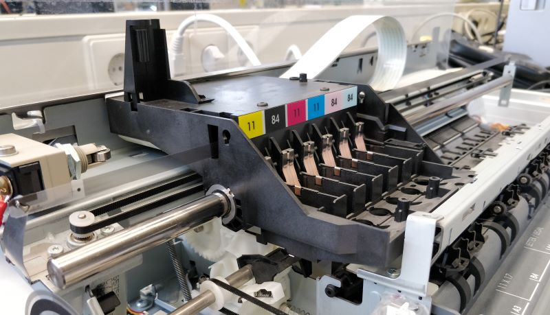
The experimental set-up consists of a current-controlled A3 printer subject to static friction, depicted in Figure 5, connected to a computer running Simulink with a sample frequency of 1 kHz. A feedback controller $C(q)$ is available, as well as an initial feedforward controller $F(q)$ of the form

i.e., a controller with velocity and acceleration as basis. The goal is to track two third-order references ${r}_{1}$ and ${r}_{2}=1.05{r}_{1}$ of length $N=4501$ samples, depicted in Figure 6, using the closed-loop scheme of Figure 1. To this end, the GP-based approach described in Section III is applied to learn a new feedforward controller $\hat{F}(q)$.

Following Procedure 1, a kernel function is defined first. The Matèrn_3/2 kernel (12) is chosen, because it is expected that static friction leads to a non-smooth function $f(\mathbf{y}_{t})$. The number of samples history and preview are defined as $n_{c}=20$ and $n_{ac}=40$ respectively.

Subsequently, 11 signals $\tilde{{r}}_{j}$ are designed as scaled variations of ${r}_{1}$, such that

Note that this leads to $\tilde{{r}}_{6}={r}_{1}\in\mathcal{R}$, i.e., the first final reference ${r}_{1}$ is used during training, unlike $r_{2}$.
Each signal $\tilde{r}_{i}\in\tilde{\mathcal{R}}$ is used as a reference for one closed-loop experiment using $C(q)$ and $F(q)$, the result of which is shown in Figure 6. The observations of $u(t)$ and $y(t)$ are used to form $\mathcal{D}$ using (6), assuming $u(\tau)=y(\tau)=0\ \forall\tau<0,\ \tau>N$. For computational reasons, the size of the dataset is reduced by only taking every $30$ rows of $Y$ and $\mathbf{u}$ into account to form $\mathcal{D}$. This leads to a dataset of $M=2970$ observations of $\mathbf{y}_{t}$ and $u(t)$. The kernel hyper-parameters are optimized by maximization of the log-marginal likelihood (see Section III-D) and the feedforward signals $\mathbf{u}_{\text{ff},1}$, $\mathbf{u}_{\text{ff},2}$ are computed with (8).

The GP-based feedforward signals are shown in Figure 7. It can be seen that the GP-based feedforward signals exhibit more complex variations than the signal resulting from $F(q)$, which may indicate that nonlinear dynamics such as position-dependent friction are learned. Moreover, the GP-based feedforward signal acts earlier to a changing reference than $F(q)$, since it has $n_{ac}=40$ samples preview, whereas $F(q)$ has no preview.

The feedforward signal is applied in closed-loop and the resulting error for ${r}_{1}$ is shown in Figure 8. The results are summarized in Table I. It can be readily seen that the tracking error is improved significantly. In particular, the linear feedforward controller $F(q)$ leads to a large tracking error around $t=2$ s since it stops at an incorrect position, as a result of static friction. The nonlinear GP-based feedforward controller $\hat{F}(q)$, on the other hand, appears to have learned these dynamics, since the error at this point in time is reduced by a factor 12.

To demonstrate the ability of the method to deal with task flexibility, Figure 9 shows the achieved performance for a reference $r_{2}$ not used during training. The tracking error is reduced to a similar extent as with $r_{1}$. This indicates that the method allows for the generation of feedforward signals for flexible tasks, provided that these tasks (or references) are sufficiently similar to the observed outputs in $\mathcal{D}$. This condition appears to be satisfied, as can be seen from Figure 6.

References

- [1] K. J. Åström, P. Hagander, and J. Sternby. Zeros of sampled systems. Automatica, 20(1):31–38, 1984.
- [2] Thomas Beckers, Dana Kulić, and Sandra Hirche. Stable Gaussian process based tracking control of Euler–Lagrange systems. Automatica, 103:390–397, May 2019.
- [3] Lennart Blanken and Tom Oomen. Kernel-based identification of non-causal systems with application to inverse model control. Automatica, 114:108830, April 2020.
- [4] Frank Boeren, Tom Oomen, and Maarten Steinbuch. Iterative motion feedforward tuning: A data-driven approach based on instrumental variable identification. Control Engineering Practice, 37:11–19, 2015.
- [5] Marc Deisenroth and Carl Rasmussen. PILCO: A Model-Based and Data-Efficient Approach to Policy Search. In Proceedings of the 28th International Conference on Machine Learning, pages 465–472, Bellevue, WA, 2011.
- [6] David J C Mackay. Information Theory, Inference, and Learning Algorithms. IEEE Transactions on Information Theory, 50(10):2544–2545, October 2004.
- [7] Charles A. Micchelli, Yuesheng Xu, and Haizhang Zhang. Universal kernels. Journal of Machine Learning Research, 7:2651–2667, 2006.
- [8] Duy Nguyen-Tuong, Jan Peters, Matthias Seeger, and Bernhard Scholkopf. Learning inverse dynamics: A comparison. In ESANN 2008 Proceedings, 16th European Symposium on Artificial Neural Networks - Advances in Computational Intelligence and Learning, pages 13–18, 2008.
- [9] Duy Nguyen-Tuong, Matthias Seeger, and Jan Peters. Model learning with local Gaussian process regression. In Advanced Robotics, volume 23, pages 2015–2034, 2009.
- [10] Panos Y. Papalambros and Douglass J Wilde. Principles of Optimal Design. Cambridge University Press, January 2017.
- [11] Gianluigi Pillonetto, Francesco Dinuzzo, Tianshi Chen, Giuseppe De Nicolao, and Lennart Ljung. Kernel methods in system identification, machine learning and function estimation: A survey. Automatica, 50(3):657–682, 2014.
- [12] C.E. Rasmussen and C.K.I. Williams. Gaussian processes for machine learning. London, England, 2006.
- [13] J. Schoukens and L. Ljung. Nonlinear system identification: A user-oriented road map. IEEE Control Systems Magazine, 39(6):28–99, 2019.
- [14] Jonas Sjöberg, Qinghua Zhang, Lennart Ljung, Albert Benveniste, Bernard Delyon, Pierre Yves Glorennec, Håkan Hjalmarsson, and Anatoli Juditsky. Nonlinear black-box modeling in system identification: a unified overview. Automatica, 31(12):1691–1724, 1995.
- [15] Peter Sollich and Christopher K. I. Williams. Understanding Gaussian Process Regression Using the Equivalent Kernel. In Lecture Notes in Computer Science (including subseries Lecture Notes in Artificial Intelligence and Lecture Notes in Bioinformatics), volume 3808 LNCS, pages 211–228. 2005.
- [16] Bharath K. Sriperumbudur, Kenji Fukumizu, and Gert R.G. Lanckriet. Universality, characteristic kernels and RKHS embedding of measures. Journal of Machine Learning Research, 12:2389–2410, 2011.
- [17] Bharath K. Sriperumbudur, Arthur Gretton, Kenji Fukumizu, Gert Lanckriet, and Bernhard Schölkopf. Injective hilbert space embeddings of probability measures. 21st Annual Conference on Learning Theory, COLT 2008, (i):111–122, 2008.
- [18] J. Van De Wijdeven and O. H. Bosgra. Using basis functions in iterative learning control: Analysis and design theory. International Journal of Control, 83(4):661–675, April 2010.