Suppressing Static Visual Cues via Normalizing Flows for Self-Supervised Video Representation Learning
Abstract
Despite the great progress in video understanding made by deep convolutional neural networks, feature representation learned by existing methods may be biased to static visual cues. To address this issue, we propose a novel method to suppress static visual cues (S2VC) based on probabilistic analysis for self-supervised video representation learning. In our method, video frames are first encoded to obtain latent variables under standard normal distribution via normalizing flows. By modelling static factors in a video as a random variable, the conditional distribution of each latent variable becomes shifted and scaled normal. Then, the less-varying latent variables along time are selected as static cues and suppressed to generate motion-preserved videos. Finally, positive pairs are constructed by motion-preserved videos for contrastive learning to alleviate the problem of representation bias to static cues. The less-biased video representation can be better generalized to various downstream tasks. Extensive experiments on publicly available benchmarks demonstrate that the proposed method outperforms the state of the art when only single RGB modality is used for pre-training. The code is available at https://github.com/mettyz/SSVC.
Introduction
Recent top-performing approaches to solving video understanding tasks are based on supervised learning with a large amount of labeled data for training. Due to the strong data fitting capacity of deep convolutional neural networks, competitive performance can be achieved for recognizing actions in videos (Carreira et al. Carreira and Zisserman 2017; Zhang et al. 2021). One of the key factors for the success may owe to the strong correlation between action class and object/background known as representation bias in (Li et al. Li, Li, and Vasconcelos 2018; Choi et al. 2019). For example, the action Riding Bike could be recognized by the presence of the object Bike and the action Swimming is recognized by the scene water. Such representation bias in action datasets may provide shortcuts to solve the data-label fitting problem. Nevertheless, the learned feature representation without proper motion modelling may be biased to static visual cues, which limits the generalization ability to recognize or detect actions requiring temporal reasoning.
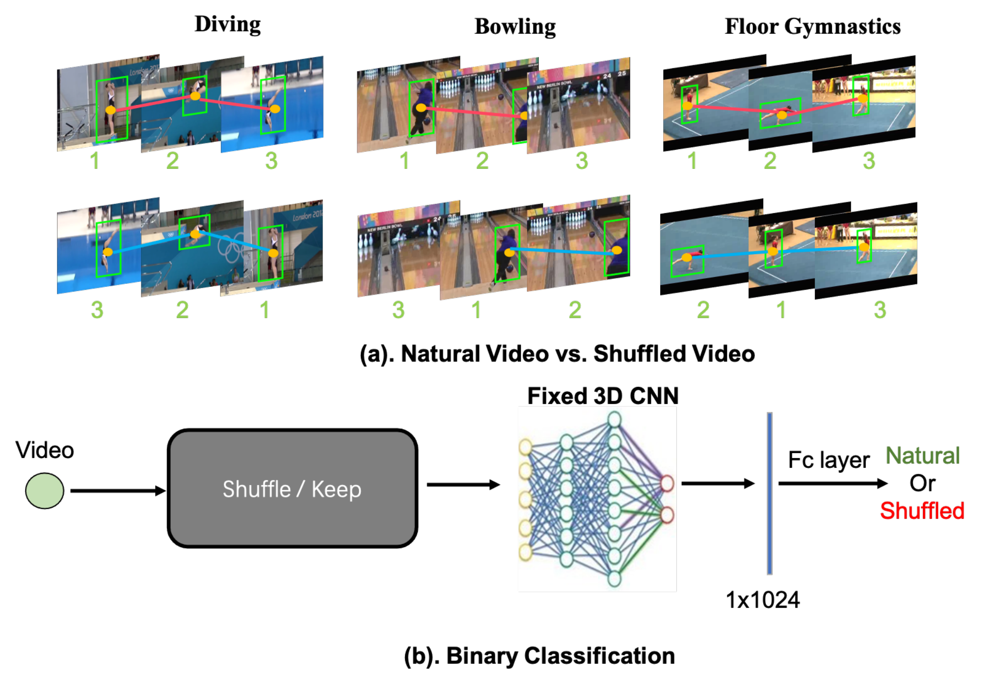
To verify this issue, we first pre-trained the R3D network (Hara et al. Hara, Kataoka, and Satoh 2018) for feature extraction in two different ways. The first one is supervised learning by using manual annotations on the UCF101 dataset (Soomro et al. Soomro, Zamir, and Shah 2012), while the second one is our self-supervised method trained on the same dataset by mitigating the representation bias. Then, the learned feature representations are evaluated on the HMDB51 dataset (Kuehne et al. 2011). The downstream task is defined as simple temporal-order (natural/shuffled) classification as illustrated in Fig. 1 to assess the generalization ability of the learned features. Fig. 1(a) shows that motion information is suppressed while static visual cues are maintained by video shuffling. Without dealing with the problem of representation bias, the supervised method performs worse than ours (73.5% v.s. 79.1% (5.6)) in the downstream task of temporal-order classification (different from the recognition task used for pre-training). This verifies our hypothesis that the generalization ability may degrade due to the misleading guidance by static visual cues.
In this paper, we propose a novel method to suppress static visual cues (S2VC) for self-supervised video representation learning, such that the representation bias is mitigated. Since the pixel space of each frame in a video is highly complicated with high dimensionality, it is not robust to directly extract static cues from it. To estimate the distribution of the pixel space, each video frame is encoded to obtain a latent vector under multivariate standard normal distribution by using normalizing flows (NF). However, when constrained to a specific video, each latent variable cannot be simply considered as one-dimensional (univariate) standard normal. We model static factors in a video as a random variable such that the conditional distribution of each latent variable becomes standard normal with shifting and scaling. The standard deviation of the conditional distribution that reflects the correlation between latent variables and static factors is then empirically estimated to select static cues. Based on probabilistic analysis, static cues are suppressed to generate motion-preserved videos by the invertibility of the NF model. Such generated videos are treated as pseudo positives for contrastive learning to mitigate the representation bias w.r.t. static visual cues.
The contributions of this work are three-fold: i. We develop a novel method to suppress static visual cues (S2VC) via normalizing flows for self-supervised video representation learning, such that the problem of representation bias is mitigated with improved generalization ability. ii. Based on probabilistic analysis, static cues are recognized and suppressed to generate motion-preserved videos for self-supervised pre-training. iii. Extensive experiments with quantitative and qualitative evaluation demonstrate the effectiveness of our method on various downstream tasks.
Related Work
Self-supervised Video Representation Learning aims at learning visual representations without using manually-annotated labels. Existing methods for video representation learning can be divided into two categories. The first one is to design pretext tasks, in which pseudo labels are automatically generated from videos for training. Representative methods along this line include predicting rotation (Jing et al. 2018), cloze (Luo et al. 2020), clip order (Misra et al. Misra, Zitnick, and Hebert 2016; Lee et al. 2017; Xu et al. 2019), playback speed (Benaim et al. 2020; Wang et al. Wang, Jiao, and Liu 2020; Yao et al. 2020; Chen et al. 2021) and so on. The second category is based on contrastive learning which has recently achieved great success in the image domain (He et al. 2020; Chen et al. 2020b; Chen et al. 2020a). The key idea is to train a feature extractor that makes a training sample similar to its generated positives and dissimilar to its negatives in the embedding space. Existing methods have been proposed to generate positive pairs by video clips sampled from the same video (Qian et al. 2021; Wang et al. 2021a; Lin et al. 2021), or codes from the same position of adjacent frames (Han et al. Han, Xie, and Zisserman 2019, Han, Xie, and Zisserman 2020a). Since additional modalities are available in videos, positive pairs can also be determined by audio (Owens and Efros 2018; Alwassel et al. 2020; Korbar et al. Korbar, Tran, and Torresani 2018), text (Sun et al. 2019b), or optical flow (Han et al. Han, Xie, and Zisserman 2020b). Though existing methods show improved performance for downstream tasks, they may be still biased to static visual cues like background or non-moving objects. To solve this problem, this paper proposes to generate motion-preserved videos by normalizing flows for less-biased representation learning.

Flow-based Generative Model is one of the widely used approaches for data generation developed with strong theory in probability (Ardizzone et al. 2019a; Dinh et al. Dinh, Krueger, and Bengio 2015; Dinh et al. Dinh, Sohl-Dickstein, and Bengio 2017). It builds on a series of invertible and differentiable functions that transforms the highly-complicated raw data distribution to the simple and interpretable standard normal distribution. This transforming sequence is called normalizing flows (NF) and is served as the foundation of invertible neural network. In recent years, NF has been successfully deployed in many applications including image generation (Kingma and Dhariwal 2018), compression (Xiao et al. 2020), colorization (Ardizzone et al. 2019c), adversarial attack (Dolatabadi et al. Dolatabadi, Erfani, and Leckie 2020), minimally invasive surgery (Ardizzone et al. 2019b), etc. To the best of our knowledge, this work is the first to suppress static cues in videos by using NF for self-supervised learning.
Methodology
The objective of our proposed method is to mitigate the representation bias brought by the strong correlation between actions and static visual cues, such that the learned features can be better generalized to different kinds of downstream tasks. The rationale is to perform probability-based video transformations that preserve motion information but suppress static visual cues (S2VC) for videos. In the following subsections, we first introduce the overall architecture of the proposed method. Then, details are given to elaborate the idea of the proposed S2VC for motion-preserved video generation via normalizing flows (NF). At last, we present the way to integrate the novel S2VC with existing self-supervised methods for video representation learning.
Overall Architecture
The training pipeline of our method is shown on the left of Fig. 2. For a given unlabelled input video , we start with two random augmentations and get and respectively, where and are randomly sampled from the basic data augmentation set . It consists of (e.g.) random cropping, random horizontal flip, color jittering and Gaussian blur. One of the randomly augmented videos is used to generate the motion-preserved video by suppressing static visual cues via normalizing flows. To mitigate the computational cost, a spatially down/up-sampling process is performed before/after the flow-based generative model. The information loss is compensated by the residual video. After that, and are fed into the 3D backbone for feature extraction to obtain and . The feature extractor is learned by minimizing the distance between and , and maximizing the distance between and other pseudo negatives from the momentum dictionary, whose features are extracted by the momentum encoder .
Suppressing Static Visual Cues
The proposed method for suppressing static visual cues is illustrated on the right of Fig. 2. For an input video, each frame is first encoded to obtain latent variables under standard normal distribution by normalizing flows (NF). Then, the motion-preserved video is generated by suppressing the less-varying latent variables (static cues) along time. Details on these two steps are provided as follows.
Encoding Video Frames via Normalizing Flows. Denote the vectorized frames in the input video as , where is the number frames and is the product of image height, width and channels. These -dimensional vectors can be considered as a sequence of observations for a random vector with the probability density . Since the dimension of the random vector is very high, it is intractable to directly estimate the density correctly. Moreover, is highly complicated due to variations like camera motions and illumination changes in videos. Without accuracy estimation of the data distribution, it not robust to extract static cues directly from the raw observed data. As a result, we propose to estimate the density of the high-dimensional random vector by normalizing flows (NF).
The idea of NF (Kobyzev et al. Kobyzev, Prince, and Brubaker 2020) is depicted on the right of Fig. 2. A sequence of simple invertible transformations (e.g., affine coupling and channel-wise permutation/convolution) maps to the latent random vector , which has the same dimension as . Denote the composition function of as , i.e., . The mapping from to is invertible and differentiable. By using , from the highly complicated distribution can be transformed to in a straightforward predefined distribution such as multivariate standard normal. To determine the parameters in the mapping function , the density is rewritten by the change-of-variables rule as,
| (1) |
where is the probability density of the latent random vector and denotes the determinant of the Jacobian matrix of partial derivatives of over . Given an image dataset (e.g., ImageNet), the model parameters are learned by maximizing the log-likelihood as follows,
| (2) |
where is the mathematical expectation.
In our method, the predefined density is set to multivariate standard normal as in (Dinh et al. Dinh, Sohl-Dickstein, and Bengio 2017), i.e., , where is a -dimensional zero vector and is a unit matrix. With the pre-trained flow model, the vectorized frames are mapped into the latent space to obtain , which are used to detect the temporally-varying patterns and extract static cues.
Motion-preserved Video Generation. Since the latent vector follows -dimensional standard normal distribution , latent variables in are independent with each other. Thus, we propose to analyze each latent variable in to identify static cues separately. If is completely random without any other information given in advance, it is obvious that the distribution of each latent variable is one-dimensional (univariate) standard normal, i.e., . Nevertheless, when the latent variable is constrained to be in a certain video, the completely random assumption is not valid.
We regard static factors (e.g., background, scene) inherited in the input video affecting the distribution of each as a random variable . For selection of static cues, the objective is to determine the density of conditioning on . Let the dependence between and be modelled by the correlation coefficient . To make the marginal density standard normal, the joint density is assumed to be two-dimensional (bivariate) normal for maximum entropy. Denote , where are the mean and variance of respectively. According to properties of normal conditional distribution (Ross 2009, 268-269), the conditional density for a given value of is still normal and can be written as,
| (3) |
This equation implies that the latent variable conditioning on an input video can be considered as standard normal random variable with shifting and scaling. With the condition , the mean and variance are changed to and , respectively.
For a latent variable strongly correlated with static factors represented by , the dependence modelled by the correlation between and is large. According to eq. (3), this means the variance is small for the latent variable encoding static cues. Notice that the variance is independent of the value of . The variance or standard deviation (STD) can be estimated empirically by the observations of the latent variable in a video. Denote the STD of the conditional density as . We propose to select the set of latent variables with small empirical STDs as static cues, i.e.,
| (4) |
where is the threshold hyperparameter used to decide whether the -th latent variable is selected or not.
Let the latent vector that preserves motion information but suppresses static cues be . For , is set to with the highest probability density, i.e., the mean of the conditional distribution as derived in eq. (3). In this way, the variance of is equal to 0 for minimum (zero) information entropy to suppress static cues. Since the marginal density takes the maximum value at , we set for by substituting into . For , motion cues are preserved by setting . Due to invertibility of the NF model , each frame in the motion-preserved video is generated by,
| (5) |
The pseudo-code of our method is given in the supplementary material. Other strategies to suppress static cues are also presented for comparison in the ablation study.
Discussion on Generative Models.
i. The generative adversarial network (GAN) has achieved success in the literature by jointly training a generator and a discriminator in an adversarial manner (Goodfellow et al. 2014; Jaiswal et al. 2018). In most existing methods based on GAN, there is no encoder to transform the image modality into the latent space. Though the generator in GAN could be used for encoding, the generation results are without explicit probability interpretation. Hence, it is difficult if not impossible to suppress static cues by the GAN approach.
ii. Different from GAN, the variational auto-encoder (VAE) (Kingma and Welling 2014; Sohn, Lee, and Yan 2015) can encode an input image to a latent vector under a multivariate normal distribution . The mean vector and standard deviation vector are determined by learnable parameters and the input image . The latent vector is obtained by randomly sampling from and can be written as , where and is the element-wise product. Due to the randomness in computing the observations of , the encoded vectors in a video may not be able to preserve the continuity of the input frames over time by using VAE. On the other hand, in the latent distribution depend on the input image , so static cues cannot be directly selected by eq. (4).
iii. By using NF, the encoded latent vector is with expressive probability interpretation, which follows multivariate standard normal distribution independent of the input image . Thanks to the differentiable property of the NF model, the encoded latent vectors preserve the continuity over time. Moreover, as experimentally shown in (Dinh et al. Dinh, Sohl-Dickstein, and Bengio 2017; Kingma et al. Kingma and Dhariwal 2018), the latent space in NF encodes semantically meaningful concepts (like smile, blond hair, male, etc. on face dataset). Because of these advantages, the flow-based approach instead of GAN and VAE is used to suppress static visual cues in our method.
Integrated with Contrastive Learning
The proposed S2VC method is integrated in the framework of contrastive learning to obtain video representations less-biased to static cues. In this work, positive pairs are constituted by the generated motion-preserved videos and corresponding inputs for self-supervised pre-training. Given a video dataset with samples for training, the loss function is defined as:
| (6) |
where denotes the temperature parameter for model learning with hard negatives (Wu et al. 2018). In each positive pair, the motion-preserved video shares the same motion information as the original one but removes static cues. By minimizing the loss function in eq. (6), the similarity of features in each positive pair is maximized. Thus, the proposed method learns discriminative video representations which simultaneously preserve motion information and suppress static cues. As an efficient and effective baseline, MoCo (He et al. 2020) is employed for contrastive learning. Furthermore, our method can serve as a powerful data augmentation technique and easily be integrated with other self-supervised learning methods, e.g., DPC in (Han et al. Han, Xie, and Zisserman 2019).
Experiments
| Method | Pretrain | Finetune | Linear Probe | ||||||
| Method | Net | Depth | Dataset | Res. | +Mod. | UCF101 | HMDB51 | UCF101 | HMDB51 |
| 3D RotNet (Jing et al. 2018) | R3D | 17 | K400 | 112 | - | 62.9 | 33.7 | 47.7 | 24.8 |
| CBT (Sun et al. 2019a) | S3D | 23 | K600+ | 112 | - | 79.5 | 44.5 | 54.0 | 29.5 |
| VCOP (Xu et al. 2019) | R(2+1)D | 26 | UCF101 | 112 | - | 72.4 | 30.9 | - | - |
| DPC (Han et al. Han, Xie, and Zisserman 2019) | R2D3D | 33 | K400 | 128 | - | 75.7 | 35.7 | - | - |
| MemDPC (Han et al. Han, Xie, and Zisserman 2020a) | R2D3D | 33 | K400 | 224 | - | 78.1 | 41.2 | 54.1 | 30.5 |
| SpeedNet (Benaim et al. 2020) | S3D | 23 | K400 | 224 | - | 81.1 | 48.8 | - | - |
| RSPNet (Chen et al. 2021) | R3D | 17 | K400 | 224 | - | 74.3 | 41.8 | - | - |
| CoCLR (Han et al. Han, Xie, and Zisserman 2020b) | S3D | 23 | K400 | 128 | F | 87.9 | 54.6 | 74.5 | 46.1 |
| IMRNet (Yu et al. 2021) | R3D | 17 | K400 | 224 | M,R | 76.8 | 45.0 | - | - |
| MoCo Baseline | S3D | 23 | UCF101 | 128 | - | 69.3 | 35.1 | 46.6 | 21.4 |
| Ours | S3D | 23 | UCF101 | 128 | - | 74.5(5.2) | 43.7(8.6) | 51.0(4.4) | 27.7(6.3) |
| Ours | S3D | 23 | K200 | 128 | - | 82.5 | 48.4 | 63.8 | 35.9 |
| Ours | R3D | 17 | UCF101 | 112 | - | 77.0 | 45.8 | 59.7 | 27.9 |
| Ours | R3D | 17 | K400 | 112 | - | 81.2 | 50.5 | 66.0 | 36.5 |
Datasets and Implementation Details
Datasets used for experiments includes UCF101 (Soomro et al. Soomro, Zamir, and Shah 2012), HMDB51 (Kuehne et al. 2011), Kinetics-400 (Kay et al. 2017), and its subset Kinetics-200 (Xie et al. 2018). We use the flow model as described in AdvFlow (Dolatabadi et al. Dolatabadi, Erfani, and Leckie 2020) for video frame encoding and generation. Two backbone networks, i.e., S3D (Xie et al. 2018) and R3D-18 (Hara et al. Hara, Kataoka, and Satoh 2018), are evaluated for contrastive learning. If not specified, we employ MoCo with S3D as the baseline and integrate our S2VC with MoCo (optimized by eq. (6) with set to 0.07). For a fair comparison, we set the input clip length and resolution as 32, for S3D and 16, for R3D. We conduct consistent augmentation for each frame in a video clip. The batch size is set as 128 and the learning rate is initialized as 1e-3. Total epochs we used for pretraining the network are 500 on UCF101, 200 on K200, and 100 on K400, respectively. Please refer to the supplementary for more implementation details.
Action Recognition
We conduct self-supervised pre-training on two settings, i.e. linear probe and finetune. For evaluation, following the common practice in (Carreira et al. Carreira and Zisserman 2017; Wang et al. 2021c), we sample each video using half-overlap sliding window, and apply ten-crops test to each video clip. Then, we average the predicted accuracy as our validation result. The results comparing with the state of the art are reported in Table 1.
Linear Probe. Follow the SimCLR (Chen et al. 2020a), we fix the weights of the pre-trained 3D CNNs and train a linear classifier after the last conv layer for 100 epochs. We can observe from the last two columns in Table 1 that our method significantly surpasses existing works that use single RGB modality for pre-training. Comparing with MemDPC (Han et al. Han, Xie, and Zisserman 2020a), the improvement by our method is up to 11.9% on UCF101 and 6.0% on HMDB51.
Finetune. We finetune the overall model for 500 epochs and show the results in Table 1. When the proposed S2VC is introduced into MoCo, with the same backbone S3D and the same pre-train dataset UCF101, it can bring 5.2% and 8.6% improvements on UCF101 and HMDB51, respectively. Due to limited computational resource, the S3D is pre-trained on K200 for only 200 epochs. The results obtained under this setting have already been better than the CBT (Sun et al. 2019a) pre-trained on the larger scale K600+, and comparable with the SpeedNet (Benaim et al. 2020) pre-trained on K400. With the R3D pre-trained on UCF101, our method also achieves competitive performance and outperforms the VCOP (Xu et al. 2019) pre-trained on the same dataset. Though the CoCLR (Han et al. Han, Xie, and Zisserman 2020b) obtain higher accuracy than ours, it needs the additional optical flow modality complementary to RGB for pre-training. Compared with the IMRNet (Yu et al. 2021) using multiple modalities in compressed videos for pre-training, our method achieves better results. The performance gains by our method over the IMRNet are 4.4% and 5.5% respectively on the two datasets by using the same backbone and pre-training dataset K400.
Video Retrieval
In this section, our method is evaluated by the video retrieval task. Following the setting in (Xu et al. 2019), we use the pre-trained 3D CNN with fixed weight as feature extractor. The training set is defined as the gallery and each 16-frame video clip from the test set is used as a query. If the category of the query appears in the retrieved -nearest neighbors, we record it as a hit during the test time. Accuracy comparison with other self-supervised learning methods on the UCF101 and HMDB51 is reported in Tables 2 and 3. When using the S3D as backbone, combining the S2VC with MoCo brings a 4.1% improvement on Top1 accuracy and 7.5% improvement on Top5 accuracy on the UCF101 dataset. For the HMDB51, the Top1 and Top5 gains are 1.7% and 5.7%, respectively. Additionally, our method outperforms the state of the art for comparison, e.g., 6.2% better than the BE (Wang et al. 2021b) under the same settings on the HMDB51. These results validate that more discriminative and generalizable representations can be extracted by our method.
| Method | Net | 1 | 5 | 10 | 20 | 50 |
|---|---|---|---|---|---|---|
| SpeedNet | S3D | 13.0 | 28.1 | 37.5 | 49.5 | 65.0 |
| VCOP | R3D | 14.1 | 30.3 | 40.4 | 51.1 | 66.5 |
| MemDPC | R3D | 20.2 | 40.4 | 52.4 | 64.7 | - |
| Pace | R3D | 23.8 | 38.1 | 46.4 | 56.6 | 69.8 |
| MoCo | S3D | 32.8 | 49.0 | 57.5 | 68.3 | 80.7 |
| Ours | S3D | 36.9 | 56.5 | 65.6 | 75.0 | 86.3 |
| Ours | R3D | 39.9 | 57.1 | 66.3 | 75.6 | 87.4 |
| Method | Net | 1 | 5 | 10 | 20 | 50 |
|---|---|---|---|---|---|---|
| VCOP | R3D | 7.6 | 22.9 | 34.4 | 48.8 | 68.9 |
| MemDPC | R3D | 7.7 | 25.7 | 40.6 | 57.7 | - |
| Pace | R3D | 9.6 | 26.9 | 41.1 | 56.1 | 76.5 |
| BE | R3D | 11.9 | 31.3 | 44.5 | 60.5 | 81.4 |
| MoCo | S3D | 13.2 | 31.8 | 44.0 | 59.7 | 80.7 |
| Ours | S3D | 14.9 | 37.5 | 51.7 | 68.3 | 84.5 |
| Ours | R3D | 18.1 | 37.9 | 51.1 | 66.0 | 84.4 |
Ablation Study

| Method | UCF101 | HMDB51 |
|---|---|---|
| MoCo | 25.4 | 11.8 |
| TFD | 29.1(3.7) | 11.6(0.2) |
| S2VC (set to random noise) | 28.7(3.3) | 12.6(0.8) |
| S2VC (shuffle - in clip) | 25.8(0.4) | 12.0(0.2) |
| S2VC (shuffle - in frame) | 29.8(4.4) | 14.0(2.2) |
| S2VC (set to 0) [default] | 30.5(5.1) | 14.9(3.1) |
Motion Threshold . In our method, in eq. (4) is an important hyperparameter to determine how many static cues are suppressed. Retrieval results of different are shown on the left of Fig. 3. These results show that as increases, the retrieval accuracy first increases, and then decreases after reaching the peak at 0.5 (the default value in this work). Interestingly, when we select as 0.8, which means only 6.5%/5.7% latent variables w.r.t motion are preserved in UCF101/HMDB51, the results are still better than small . This indicates the importance of suppressing sufficient static cues and keeping conspicuous motion information for action recognition. We also visualize the generation results of different on the right of Fig. 3. If is too small, the effect for suppressing static cues is insufficient. In contrast, for too large , useful action cues may also be suppressed.
Strategy for Suppressing Static Cues. In this experiment, we evaluate different Strategies for suppressing static cues. First, we compare with a simple thresholding frame difference (TFD) method by pixel-level operation. Similar to our method, each frame in a video is reshaped to in the TFD. Then, the top pixels with the largest STD along the time dimension are persevered (approximately equal to the amount of the preserved motion cues in the proposed S2VC when ). Besides the TFD, three variants of the proposed S2VC to determine the suppressed latent variables are evaluated: (a) set to random noise: set latent variables in to normal noise for the first frame and keep them unchanged for other frames. (b) shuffle - in clip: randomly shuffle each latent variable in between frames of a video. (c) shuffle - in frame: randomly shuffle each latent variable in within a frame. For fair comparison, we pre-train all the methods with the S3D on the UCF101 for 100 epochs.
Retrieval results are shown in Table 4. We have the following observations: i. The in-clip shuffle method brings little gain to the baseline model, since the channels already have similar values (small at standard deviation). ii. All methods that strongly disturb the static cues show great improvement to the baseline model. iii. TFD surpass the MoCo baseline on UCF101 but perform worse on HMDB51. This indicates that it is not robust and hard to generalize to a new dataset by simply detecting motion according to pixel level difference. iv. It performs the best by setting all latent variables in to zero. Recall that zero suppressed latent variables refers to the minimum information entropy with the highest probability. Other suppressing methods are not the most likely or with randomness to carry static information. As a result, we use the S2VC (set to 0) as default.
Analysis on Suppressing Effects
Intra-class similarity of different samples. Given , we investigate the visual similarity over different samples in the same action category. Specifically, we randomly select ten classes from UCF101/HMDB51 and sample a subset of video clips for each category. Then, we measure the cosine similarity of different samples frame-by-frame with the latent vector and the motion-preserved vector , respectively. As frames in the same class may have a similar scene but large difference in moving regions, the cosine similarity is smaller if the latent vectors contain less static visual cues. The decreased similarity of compare with shown in Fig. 4 is aligned with the above analysis. This phenomenon demonstrates that our method reduces the intra-class similarity of static object/background significantly, which ensures that the generated motion-preserved videos are less biased to static cues. We also observe that different categories show widely varied ratios over v.s. , which means action classes have various similarities on static cues.


Visualization of the suppressing quality. More intuitively, we compare the generation of motion-preserved videos with minor/intense camera motion. As shown in Fig. 5, the generation is more robust to noise like camera movement and is able to focus on the most salient motion by suppressing static cues in the latent space encoded by the NF.
Analysis on Performance Improvement
Relative Improvement over Static Classification. As our method suppress static visual cues, it may bring negative impact to classes that have a high correlation with non-moving object or background. To study the correlation between the temporal dependency of actions and the performance gain brought by our method, we plot the class-level relative performance improvement in Fig. 6. In this experiment, we first train a randomly initialized S3D baseline using static videos (stacked copy images). Since the stacked duplicate images provide no temporal information, the performance of the baseline model indicates how much a category depends on the static visual cues. The plot shows that although there exist some classes that our method leads to a worse result, the overall performance is better. Moreover, there is a clear negative relationship between relative gain and baseline performance, which suggests that the superiority of our method is mainly coming from precisely identifying actions with high temporal dependency. We also find that our model shows a stronger negative correlation compared with MoCo.


Salient Regions Compared with Optical Flow. In this experiment, we visualize the energy of the last convolutional layer with the Class-Activation Map (CAM) technique (Zhou et al. 2016). We sample from the HMDB51 instead of the UCF101 used for pre-training to show the generalizability. We also visualize the optical flow for reference, which indicates the significant motion cues in the video. The results are depicted in Fig. 7. From these samples, we find a strong correlation between highly activated regions and the dominant mover in the scene. The network pre-trained with the S2VC tends to focus more on the moving object. For example, in the second row, only our method concentrates on the two boys dribbling the ball on either side separately.
Conclusion
In this paper, we present a novel method to suppress static visual cues (S2VC), which mitigates the representation bias over less-moving object/background in videos. Due to the difficulty in estimating the pixel-level distribution, video frames are encoded to a latent space under multivariate standard normal distribution by normalizing flows. Then, less-varying latent variables along time are selected as static cues based on probabilistic analysis and suppressed to generate motion-preserved videos. The proposed S2VC is integrated with the self-supervised learning framework to extract video representations that focus more on motion cues. Extensive experiments with visualization validate that features learned by our method pay more attention to moving objects and can be better generalized to different downstream tasks.
Acknowledgement
This work was supported partially by National Natural Science Foundation of China (No. 61906218), Guangdong Basic and Applied Basic Research Foundation (No. 2020A1515011497) and Science and Technology Program of Guangzhou (No. 202002030371).
References
- Alwassel et al. (2020) Alwassel, H.; Mahajan, D.; Korbar, B.; Torresani, L.; Ghanem, B.; and Tran, D. 2020. Self-supervised learning by cross-modal audio-video clustering. In NeurIPS.
- Ardizzone et al. (2019a) Ardizzone, L.; Kruse, J.; Rother, C.; and Köthe, U. 2019a. Analyzing Inverse Problems with Invertible Neural Networks. In ICLR.
- Ardizzone et al. (2019b) Ardizzone, L.; Kruse, J.; Rother, C.; and Köthe, U. 2019b. Analyzing Inverse Problems with Invertible Neural Networks. In ICLR.
- Ardizzone et al. (2019c) Ardizzone, L.; Lüth, C.; Kruse, J.; Rother, C.; and Köthe, U. 2019c. Guided image generation with conditional invertible neural networks. arXiv preprint arXiv:1907.02392.
- Benaim et al. (2020) Benaim, S.; Ephrat, A.; Lang, O.; Mosseri, I.; Freeman, W. T.; Rubinstein, M.; Irani, M.; and Dekel, T. 2020. Speednet: Learning the speediness in videos. In CVPR, 9922–9931.
- Carreira and Zisserman (2017) Carreira, J.; and Zisserman, A. 2017. Quo Vadis, Action Recognition? A New Model and the Kinetics Dataset. In CVPR, 4724–4733.
- Chen et al. (2021) Chen, P.; Huang, D.; He, D.; Long, X.; Zeng, R.; Wen, S.; Tan, M.; and Gan, C. 2021. RSPNet: Relative Speed Perception for Unsupervised Video Representation Learning. In AAAI, 1045–1053.
- Chen et al. (2020a) Chen, T.; Kornblith, S.; Norouzi, M.; and Hinton, G. 2020a. A simple framework for contrastive learning of visual representations. In ICML, 1597–1607.
- Chen et al. (2020b) Chen, X.; Fan, H.; Girshick, R.; and He, K. 2020b. Improved baselines with momentum contrastive learning. arXiv preprint arXiv:2003.04297.
- Choi et al. (2019) Choi, J.; Gao, C.; Messou, J. C.; and Huang, J.-B. 2019. Why Can’t I Dance in the Mall? Learning to Mitigate Scene Bias in Action Recognition. In NeurIPS, 853–865.
- Dinh, Krueger, and Bengio (2015) Dinh, L.; Krueger, D.; and Bengio, Y. 2015. Nice: Non-linear independent components estimation. In ICLR (Workshop).
- Dinh, Sohl-Dickstein, and Bengio (2017) Dinh, L.; Sohl-Dickstein, J.; and Bengio, S. 2017. Density estimation using real nvp. In ICLR.
- Dolatabadi, Erfani, and Leckie (2020) Dolatabadi, H. M.; Erfani, S.; and Leckie, C. 2020. AdvFlow: Inconspicuous Black-box Adversarial Attacks using Normalizing Flows. In NeurIPS.
- Goodfellow et al. (2014) Goodfellow, I. J.; Pouget-Abadie, J.; Mirza, M.; Xu, B.; Warde-Farley, D.; Ozair, S.; Courville, A. C.; and Bengio, Y. 2014. Generative Adversarial Nets. In NeurIPS, 2672–2680.
- Han, Xie, and Zisserman (2019) Han, T.; Xie, W.; and Zisserman, A. 2019. Video representation learning by dense predictive coding. In ICCV (Workshop).
- Han, Xie, and Zisserman (2020a) Han, T.; Xie, W.; and Zisserman, A. 2020a. Memory-augmented dense predictive coding for video representation learning. In ECCV, 312–329.
- Han, Xie, and Zisserman (2020b) Han, T.; Xie, W.; and Zisserman, A. 2020b. Self-supervised Co-Training for Video Representation Learning. In NeurIPS.
- Hara, Kataoka, and Satoh (2018) Hara, K.; Kataoka, H.; and Satoh, Y. 2018. Can Spatiotemporal 3D CNNs Retrace the History of 2D CNNs and ImageNet? In CVPR, 6546–6555.
- He et al. (2020) He, K.; Fan, H.; Wu, Y.; Xie, S.; and Girshick, R. 2020. Momentum contrast for unsupervised visual representation learning. In CVPR, 9729–9738.
- Jaiswal et al. (2018) Jaiswal, A.; AbdAlmageed, W.; Wu, Y.; and Natarajan, P. 2018. Bidirectional Conditional Generative Adversarial Networks. In ACCV, 216–232.
- Jing et al. (2018) Jing, L.; Yang, X.; Liu, J.; and Tian, Y. 2018. Self-supervised spatiotemporal feature learning via video rotation prediction. arXiv preprint arXiv:1811.11387.
- Kay et al. (2017) Kay, W.; Carreira, J.; Simonyan, K.; Zhang, B.; Hillier, C.; Vijayanarasimhan, S.; Viola, F.; Green, T.; Back, T.; Natsev, P.; et al. 2017. The kinetics human action video dataset. arXiv preprint arXiv:1705.06950.
- Kingma and Dhariwal (2018) Kingma, D. P.; and Dhariwal, P. 2018. Glow: Generative flow with invertible 1x1 convolutions. In NeurIPS.
- Kingma and Welling (2014) Kingma, D. P.; and Welling, M. 2014. Auto-Encoding Variational Bayes. In ICLR.
- Kobyzev, Prince, and Brubaker (2020) Kobyzev, I.; Prince, S. J.; and Brubaker, M. A. 2020. Normalizing Flows: An Introduction and Review of Current Methods. IEEE TPAMI, 1–1.
- Korbar, Tran, and Torresani (2018) Korbar, B.; Tran, D.; and Torresani, L. 2018. Cooperative learning of audio and video models from self-supervised synchronization. In NeurIPS, 7774–7785.
- Kuehne et al. (2011) Kuehne, H.; Jhuang, H.; Garrote, E.; Poggio, T.; and Serre, T. 2011. HMDB: a large video database for human motion recognition. In ICCV, 2556–2563.
- Lee et al. (2017) Lee, H.-Y.; Huang, J.-B.; Singh, M.; and Yang, M.-H. 2017. Unsupervised representation learning by sorting sequences. In ICCV, 667–676.
- Li, Li, and Vasconcelos (2018) Li, Y.; Li, Y.; and Vasconcelos, N. 2018. Resound: Towards action recognition without representation bias. In ECCV, 513–528.
- Lin et al. (2021) Lin, Y.; Wang, J.; Zhang, M.; and Ma, A. J. 2021. Learning Spatio-temporal Representation by Channel Aliasing Video Perception. In Proceedings of the 29th ACM International Conference on Multimedia, 2317–2325.
- Luo et al. (2020) Luo, D.; Liu, C.; Zhou, Y.; Yang, D.; Ma, C.; Ye, Q.; and Wang, W. 2020. Video cloze procedure for self-supervised spatio-temporal learning. In AAAI, 11701–11708.
- Misra, Zitnick, and Hebert (2016) Misra, I.; Zitnick, C. L.; and Hebert, M. 2016. Shuffle and learn: unsupervised learning using temporal order verification. In ECCV, 527–544.
- Owens and Efros (2018) Owens, A.; and Efros, A. A. 2018. Audio-visual scene analysis with self-supervised multisensory features. In ECCV, 631–648.
- Qian et al. (2021) Qian, R.; Meng, T.; Gong, B.; Yang, M.; Wang, H.; Belongie, S. J.; and Cui, Y. 2021. Spatiotemporal Contrastive Video Representation Learning. In CVPR, 6964–6974.
- Ross (2009) Ross, S. M., ed. 2009. A First Course in Probability. Upper Saddle River, N.J.: Pearson Prentice Hall, eighth edition.
- Sohn, Lee, and Yan (2015) Sohn, K.; Lee, H.; and Yan, X. 2015. Learning Structured Output Representation using Deep Conditional Generative Models. In NeurIPS, 3483–3491.
- Soomro, Zamir, and Shah (2012) Soomro, K.; Zamir, A. R.; and Shah, M. 2012. UCF101: A dataset of 101 human actions classes from videos in the wild. arXiv preprint arXiv:1212.0402.
- Sun et al. (2019a) Sun, C.; Baradel, F.; Murphy, K.; and Schmid, C. 2019a. Learning video representations using contrastive bidirectional transformer. arXiv preprint arXiv:1906.05743.
- Sun et al. (2019b) Sun, C.; Myers, A.; Vondrick, C.; Murphy, K.; and Schmid, C. 2019b. Videobert: A joint model for video and language representation learning. In ICCV, 7464–7473.
- Wang et al. (2021a) Wang, J.; Gao, Y.; Li, K.; Jiang, X.; Guo, X.; Ji, R.; and Sun, X. 2021a. Enhancing unsupervised video representation learning by decoupling the scene and the motion. In AAAI.
- Wang et al. (2021b) Wang, J.; Gao, Y.; Li, K.; Lin, Y.; Ma, A. J.; and Sun, X. 2021b. Removing the Background by Adding the Background: Towards Background Robust Self-supervised Video Representation Learning. In CVPR.
- Wang, Jiao, and Liu (2020) Wang, J.; Jiao, J.; and Liu, Y.-H. 2020. Self-supervised video representation learning by pace prediction. In ECCV, 504–521.
- Wang et al. (2021c) Wang, J.; Lin, Y.; Zhang, M.; Gao, Y.; and Ma, A. J. 2021c. Multi-level Temporal Dilated Dense Prediction for Action Recognition. IEEE Transactions on Multimedia.
- Wu et al. (2018) Wu, Z.; Xiong, Y.; Yu, S. X.; and Lin, D. 2018. Unsupervised feature learning via non-parametric instance discrimination. In CVPR, 3733–3742.
- Xiao et al. (2020) Xiao, M.; Zheng, S.; Liu, C.; Wang, Y.; He, D.; Ke, G.; Bian, J.; Lin, Z.; and Liu, T.-Y. 2020. Invertible image rescaling. In ECCV, 126–144.
- Xie et al. (2018) Xie, S.; Sun, C.; Huang, J.; Tu, Z.; and Murphy, K. 2018. Rethinking Spatiotemporal Feature Learning: Speed-Accuracy Trade-offs in Video Classification. In ECCV, 318–335.
- Xu et al. (2019) Xu, D.; Xiao, J.; Zhao, Z.; Shao, J.; Xie, D.; and Zhuang, Y. 2019. Self-supervised spatiotemporal learning via video clip order prediction. In CVPR, 10334–10343.
- Yao et al. (2020) Yao, Y.; Liu, C.; Luo, D.; Zhou, Y.; and Ye, Q. 2020. Video playback rate perception for self-supervised spatio-temporal representation learning. In CVPR, 6548–6557.
- Yu et al. (2021) Yu, Y.; Lee, S.; Kim, G.; and Song, Y. 2021. Self-Supervised Learning of Compressed Video Representations. In ICLR.
- Zhang et al. (2021) Zhang, D. J.; Li, K.; Chen, Y.; Wang, Y.; Chandra, S.; Qiao, Y.; Liu, L.; and Shou, M. Z. 2021. MorphMLP: A Self-Attention Free, MLP-Like Backbone for Image and Video. arXiv preprint arXiv:2111.12527.
- Zhou et al. (2016) Zhou, B.; Khosla, A.; Lapedriza, A.; Oliva, A.; and Torralba, A. 2016. Learning deep features for discriminative localization. In CVPR, 2921–2929.