跳到论文正文
W Papers独立论文阅读器 arXiv:2112.03616 论文正文 计算阅读时间 · 0%
引用这篇论文根据当前论文元数据生成,正式投稿前建议核对。


License: CC Zero
arXiv:2112.03616v1 [math.NA] 07 Dec 2021
\catchline

Improved uniform error bounds on time-splitting methods for the long-time dynamics of the Dirac equation with small potentials

Weizhu Bao Address: Department of Mathematics, National University of Singapore, Singapore, 119076, Singapore
matbaowz@nus.edu.sg
   Yue Feng Address: Department of Mathematics, National University of Singapore, Singapore, 119076, Singapore
fengyue@u.nus.edu
   Jia Yin Address: Applied Mathematics and Computational Research (AMCR) Division, Lawrence Berkeley National Laboratory, Berkeley, CA 94720, USA
jiayin@lbl.gov
Received  (Day Month Year); Revised  (Day Month Year)
Abstract

We establish improved uniform error bounds on time-splitting methods for the long-time dynamics of the Dirac equation with small electromagnetic potentials characterized by a dimensionless parameter ε∈(0,1]\varepsilon\in(0,1] representing the amplitude of the potentials. We begin with a semi-discritization of the Dirac equation in time by a time-splitting method, and then followed by a full-discretization in space by the Fourier pseudospectral method. Employing the unitary flow property of the second-order time-splitting method for the Dirac equation, we prove uniform error bounds at C⁡(t)​τ2C(t)\tau^{2} and C⁡(t)​(hm+τ2)C(t)(h^{m}+\tau^{2}) for the semi-discretization and full-discretization, respectively, for any time t∈[0,Tε]t\in[0,T_{\varepsilon}] with Tε=T/εT_{\varepsilon}=T/\varepsilon for T>0T>0, which are uniformly for ε∈(0,1]\varepsilon\in(0,1], where τ\tau is the time step, hh is the mesh size, m≥2m\geq 2 depends on the regularity of the solution, and C⁡(t)=C0+C1​ε​t≤C0+C1​TC(t)=C_{0}+C_{1}\varepsilon t\leq C_{0}+C_{1}T grows at most linearly with respect to tt with C0≥0C_{0}\geq 0 and C1>0C_{1}>0 two constants independent of tt, hh, τ\tau and ε\varepsilon. Then by adopting the regularity compensation oscillation (RCO) technique which controls the high frequency modes by the regularity of the solution and low frequency modes by phase cancellation and energy method, we establish improved uniform error bounds at O⁡(ε​τ2)O(\varepsilon\tau^{2}) and O⁡(hm+ε​τ2)O(h^{m}+\varepsilon\tau^{2}) for the semi-discretization and full-discretization, respectively, up to the long-time TεT_{\varepsilon}. Numerical results are reported to confirm our error bounds and to demonstrate that they are sharp. Comparisons on the accuracy of different time discretizations for the Dirac equation are also provided.

keywords
Dirac equation; long-time dynamics; time-splitting methods; improved uniform error bound; regularity compensation oscillation.
{history}\comby

(xxxxxxxxxx)

\ccode

AMS Subject Classification: 35Q41, 65M70, 65N35, 81Q05

1 Introduction

In this paper, we consider the Dirac equation in one or two dimensions (1D or 2D), which can be represented in the two-component form with wave function Φ:=Φ⁡(t,𝐱)=(ϕ1​(t,𝐱),ϕ2​(t,𝐱))T∈ℂ2\Phi:=\Phi(t,{\mathbf{x}})=(\phi_{1}(t,{\mathbf{x}}),\phi_{2}(t,{\mathbf{x}}))^{T}\in\mathbb{C}^{2} as[13, 14, 33]

i∂tΦ=(−i∑j=1dσj∂j+σ3)Φ+ε(V(𝐱)I2−∑j=1dAj(𝐱)σj)Φ,𝐱∈Ω,i\partial_{t}\Phi=\left(-i\sum_{j=1}^{d}\sigma_{j}\partial_{j}+\sigma_{3}\right)\Phi+\varepsilon\left(V(\mathbf{x})I_{2}-\sum_{j=1}^{d}A_{j}(\mathbf{x})\sigma_{j}\right)\Phi,\quad\mathbf{x}\in\Omega, (1)

where Ω⊂ℝd\Omega\subset\mathbb{R}^{d} (d=1,2)(d=1,2) is a bounded domain equipped with periodic boundary condition. Here, i=−1i=\sqrt{-1}, t≥0t\geq 0 is time, 𝐱=(x1,…,xd)T∈ℝd\mathbf{x}=(x_{1},\ldots,x_{d})^{T}\in\mathbb{R}^{d}, ∂j=∂∂xj(j=1,…,d)\partial_{j}=\frac{\partial}{\partial x_{j}}(j=1,\ldots,d), ε∈(0,1]\varepsilon\in(0,1] is a dimensionless parameter, V⁡(𝐱)V(\mathbf{x}) and Aj​(𝐱)A_{j}({\mathbf{x}}) are the given real-valued time-independent electric and magnetic potentials, respectively. I2I_{2} is the 2×22\times 2 identity matrix, and σ1,σ2,σ3\sigma_{1},\sigma_{2},\sigma_{3} are the Pauli matrices defined as

σ1=(0 11 0),σ2=(0−ii 0),σ3=(1 00−1).\sigma_{1}=\begin{pmatrix}0&\ \ 1\\ 1&\ \ 0\end{pmatrix},\quad\sigma_{2}=\begin{pmatrix}0&\ \ -i\\ i&\ \ 0\end{pmatrix},\quad\sigma_{3}=\begin{pmatrix}1&\ \ 0\\ 0&\ \ -1\end{pmatrix}. (2)

In order to study the dynamics of the Dirac equation (1), the initial condition is taken as

Φ⁡(t=0,𝐱)=Φ0​(𝐱),𝐱∈Ω¯.\Phi(t=0,\mathbf{x})=\Phi_{0}(\mathbf{x}),\quad{\bf x}\in\overline{\Omega}. (3)

For the Dirac equation (1) with ε=1\varepsilon=1, i.e., the classical regime, there are comprehensive analytical and numerical results in the literatures. Along the analytical front, for the existence and multiplicity of bound states and/or standing wave solutions, we refer to Refs. \refciteES,GGT,Gross and references therein. In the numerical aspect, different numerical methods have been proposed and analyzed, such as the finite difference time domain (FDTD) methods[4, 28], exponential wave integrator Fourier pseudospectral (EWI-FP) method[4, 5], and time-splitting Fourier pseudospectral (TSFP) method[7, 8], etc. For more details related to the numerical schemes, we refer to Refs. \refciteBSG,FLB,Gosse,GSX,MK and references therein.

However, to our knowledge, much less research has been done for the long-time dynamics when ε∈(0,1]\varepsilon\in(0,1]. With a small ε\varepsilon, we can study the long-time dynamics of the Dirac equation (1) for t∈[0,Tε]t\in[0,T_{\varepsilon}] with Tε:=T/εT_{\varepsilon}:=T/\varepsilon for T>0T>0, while either ε\varepsilon or TT can be fixed (or changed) in the analysis. When ε∈(0,1]\varepsilon\in(0,1] is fixed, e.g. ε=1\varepsilon=1, we would like to investigate how the errors of different numerical schemes perform for t∈[0,Tε]t\in[0,T_{\varepsilon}] with increasing TT. On the other hand, when TT is fixed, we are interested in analyzing the dependency of errors for different numerical methods on the parameter ε\varepsilon for t∈[0,Tε]t\in[0,T_{\varepsilon}]. In our recent works, we examined the long-time error bounds for finite difference time domain (FDTD) methods and finite difference Fourier pseudospectral (FDFP) methods, where the finite difference was applied to discretize the Dirac equation (1) in time and different discretizations were taken in space. We rigorously proved that the FDTD methods share an error bound at O⁡(h2ε+τ2ε)O(\frac{h^{2}}{\varepsilon}+\frac{\tau^{2}}{\varepsilon}) up to the long-time TεT_{\varepsilon} with hh the spatial mesh size and τ\tau the temporal step size, while the FDFP methods exhibit an error bound at O⁡(hm+τ2ε)O(h^{m}+\frac{\tau^{2}}{\varepsilon}) up to the long-time[18]. The uniform spatial error bound with respect to ε\varepsilon for the FDFP methods indicate that these methods have better spatial resolution than the FDTD methods to solve the Dirac equation with small potentials in the long-time regime. Nevertheless, both types of methods face severe numerical burdens when ε→0+\varepsilon\to 0^{+} due to the ε\varepsilon-dependence of the temporal error. To deal with this problem, we adopted the exponential wave integrator (EWI) method for time discretization, and obtained a uniform error bound at O⁡(hm+τ2)O(h^{m}+\tau^{2}) up to the long-time[19].

To further improve the temporal error for ε∈(0,1]\varepsilon\in(0,1], we consider the time-splitting methods, which have been widely used to numerically solve dispersive partial differential equations (PDEs)[1, 21, 26, 29]. It has been proved that the temporal error bounds grow linearly when the time-splitting methods are applied to the Maxwell’s equations[11, 12]. In addition, the unitary flow property of the time-splitting methods contributes to the time-dependent uniform error bounds for the Schrödinger equation and the improved uniform error bounds for the Schrödinger/nonlinear Schrödinger equation with the help of the regularity compensation oscillation (RCO) technique[2, 3]. This improves the analysis in the previous studies and obtains surprising error estimates for the time-splitting methods[2, 3]. The aim of this paper is to establish the improved uniform error bounds on time-splitting methods for the long-time dynamics of the Dirac equation with small potentials. First, we prove a uniform error bound where the error constant grows linearly with respect to the time tt. Based on the error bound, for a given accuracy δ0\delta_{0} and time step τ\tau, the second order time-splitting (Strang splitting) could be applied to simulate the dynamics of the Dirac equation up to O⁡(δ0/τ2)O(\delta_{0}/\tau^{2}) when ε=1\varepsilon=1, i.e., the smaller the time step τ\tau, the longer the dynamics that can be calculated. Then by employing the RCO technique[2, 3], we establish improved uniform error bounds at O⁡(ε​τ2+τ0m)O(\varepsilon\tau^{2}+\tau_{0}^{m}) and O⁡(hm+ε​τ2+τ0m)O(h^{m}+\varepsilon\tau^{2}+\tau_{0}^{m}) for the semi-discretization and full-discretization, respectively, for the Dirac equation with O⁡(ε)O(\varepsilon)-potentials up to the long-time at O⁡(1/ε)O(1/\varepsilon). In the error bounds, m≥2m\geq 2 depends on the regularity of the exact solution and τ0∈(0,1)\tau_{0}\in(0,1) is a fixed chosen parameter. When the solution is smooth, i.e. m→∞m\to\infty, then the error bounds collapse to O⁡(ε​τ2)O(\varepsilon\tau^{2}) and O⁡(hm+ε​τ2)O(h^{m}+\varepsilon\tau^{2}) for the semi-discretization and full-discretization, respectively.

The rest of this paper is organized as follows. In Section 2, the second-order time-splitting methods including the semi-discretization and full-discretization for the long-time dynamics of the Dirac equation with small potentials are presented. In Section 3, uniform error bounds for the time-splitting methods are established up to the long-time at O⁡(1/ε)O(1/\varepsilon) and the errors are shown to grow linearly with respect to the time tt. In Section 4, we prove the improved uniform error bounds rigorously by adopting the RCO technique. Extensive numerical results are reported in Section 5. Finally, some conclusions are drawn in Section 6. Throughout this paper, we adopt the notation A≲BA\lesssim B to represent that there exists a generic constant C>0C>0, which is independent of the mesh size hh and time step τ\tau as well as the parameter ε\varepsilon such that |A|≤C​B|A|\leq CB.

2 The time-splitting methods

For simplicity, in the following sections, we focus on the Dirac equation (1) in 1D, i.e., d=1d=1 in (1), for the numerical methods and corresponding analysis. The methods and results can be easily generalized to (1) in 2D, i.e., d=2d=2, and to the four-component Dirac equation given in Refs. \refciteBCJT and \refciteBCJY.

The Dirac equation (1) in 1D on the bounded computational domain Ω=(a,b)\Omega=(a,b) with periodic boundary condition collapses to

i∂tΦ=(−iσ1∂x+σ3)Φ+ε(V(x)I2−A1(x)σ1)Φ,x∈Ω,t>0,\displaystyle i\partial_{t}\Phi=(-i\sigma_{1}\partial_{x}+\sigma_{3})\Phi+\varepsilon(V(x)I_{2}-A_{1}(x)\sigma_{1})\Phi,\qquad x\in\Omega,\quad t>0, (4)
Φ⁡(t,a)=Φ⁡(t,b),t≥0;Φ⁡(0,x)=Φ0​(x),x∈Ω¯,\displaystyle\Phi(t,a)=\Phi(t,b),\quad t\geq 0;\qquad\Phi(0,x)=\Phi_{0}(x),\quad x\in\overline{\Omega}, (5)

where Φ:=Φ⁡(t,x)\Phi:=\Phi(t,x) and Φ0​(a)=Φ0​(b)\Phi_{0}(a)=\Phi_{0}(b).

2.1 The semi-discretization

Define the operators

𝐓:=−σ1∂x−iσ3,𝐕:=−i(V(x)I2−A1(x)σ1),\mathbf{T}:=-\sigma_{1}\partial_{x}-i\sigma_{3},\quad\mathbf{V}:=-i(V(x)I_{2}-A_{1}(x)\sigma_{1}), (6)

then (4) can be expressed by

∂tΦ⁡(t,x)=(𝐓+ε​𝐕)​Φ​(t,x),x∈Ω,t>0.\partial_{t}\Phi(t,x)=(\mathbf{T}+\varepsilon\mathbf{V})\Phi(t,x),\ x\in\Omega,\ t>0. (7)

Take a time step size τ>0\tau>0 and denote the time grids as tn=n​τt_{n}=n\tau for n=0,1,…n=0,1,\ldots. As both 𝐓\mathbf{T} and 𝐕\mathbf{V} are time-independent, the solution to (7) with (5) can be propagated through

Φ(tn+1,x)=eτ⁡(𝐓+ε​𝐕)Φ(tn,x),n=0,1,….\Phi(t_{n+1},x)=e^{\tau(\mathbf{T}+\varepsilon\mathbf{V})}\Phi(t_{n},x),\quad n=0,1,\ldots. (8)

To approximate the operator eτ⁡(𝐓+ε​𝐕)e^{\tau(\mathbf{T}+\varepsilon\mathbf{V})}, we apply the second-order time-splitting (Strang splitting)[32], which gives

eτ⁡(𝐓+ε​𝐕)≈eτ2​𝐓​eε​τ​𝐕​eτ2​𝐓.e^{\tau(\mathbf{T}+\varepsilon\mathbf{V})}\approx e^{\frac{\tau}{2}\mathbf{T}}e^{\varepsilon\tau\mathbf{V}}e^{\frac{\tau}{2}\mathbf{T}}. (9)

Therefore, the semi-discretization of the Dirac equation (4) via Strang splitting can be expressed as

Φ[n+1](x)=𝒮τ(Φ[n](x)):=eτ2​𝐓eε​τ​𝐕eτ2​𝐓Φ[n](x),n=0,1,…,\Phi^{[n+1]}(x)=\mathcal{S}_{\tau}(\Phi^{[n]}(x)):=e^{\frac{\tau}{2}\mathbf{T}}e^{\varepsilon\tau\mathbf{V}}e^{\frac{\tau}{2}\mathbf{T}}\Phi^{[n]}(x),\quad n=0,1,\ldots, (10)

where we take the initial condition Φ[0]​(x):=Φ0​(x)\Phi^{[0]}(x):=\Phi_{0}(x) for x∈Ω¯x\in\overline{\Omega}. Here, Φ[n]​(x)\Phi^{[n]}(x) is the approximation of Φ⁡(tn,x)\Phi(t_{n},x).

2.2 The full-discretization

By noticing the definition of 𝐕\mathbf{V} in (6), it is easy to derive that

eε​τ​𝐕​Φ​(t,x)=e−i​ε​τ​(V⁡(x)​I2−A1​(x)​σ1)​Φ​(t,x),x∈Ω¯,t>0.e^{\varepsilon\tau\mathbf{V}}\Phi(t,x)=e^{-i\varepsilon\tau\left(V(x)I_{2}-A_{1}(x)\sigma_{1}\right)}\Phi(t,x),\quad x\in\overline{\Omega},\quad t>0. (11)

On the other hand, to get eτ​𝐓​Φ​(t,x)e^{\tau\mathbf{T}}\Phi(t,x), we can discretize (7) in space by the Fourier spectral method, and then it is possible to integrate the operator analytically in the phase space. We take M+1M+1 uniformly sampled grid points in Ω¯\overline{\Omega} with MM a positive even integer

xj=a+jh,h=b−aM,j=0,1,…,M,x_{j}=a+jh,\quad h=\frac{b-a}{M},\quad j=0,1,\ldots,M, (12)

and we denote the sets XMX_{M}, YMY_{M}, ZMZ_{M} as

XM={U=(U0,U1,…,UM)T|Uj∈ℂ2,j=0,1,…,M,U0=UM},\displaystyle X_{M}=\left\{U=(U_{0},U_{1},\ldots,U_{M})^{T}~|~U_{j}\in\mathbb{C}^{2},\,j=0,1,\ldots,M,\,U_{0}=U_{M}\right\},
YM=ZM×ZM,ZM=span⁡{ϕl​(x)=ei​μl​(x−a),l∈𝒯M},\displaystyle Y_{M}=Z_{M}\times Z_{M},\quad Z_{M}={\rm{span}}\{\phi_{l}(x)=e^{i\mu_{l}(x-a)},\,l\in\mathcal{T}_{M}\},

where the index set 𝒯M={l|l=−M/2,−M/2+1,…,M/2−1}\mathcal{T}_{M}=\{l~|~l=-M/2,-M/2+1,\ldots,M/2-1\}, and μl=2​π​l/(b−a)\mu_{l}=2\pi l/(b-a) for l∈𝒯Ml\in\mathcal{T}_{M}. The projection operator PM:(L2​(Ω))2→YMP_{M}:\left(L^{2}(\Omega)\right)^{2}\rightarrow Y_{M} is defined as

(PM​U)​(x):=∑l∈𝒯MU^l​ei​μl​(x−a),U⁡(x)∈(L2​(Ω))2,\left(P_{M}U\right)(x):=\sum_{l\in\mathcal{T}_{M}}\widehat{U}_{l}e^{i\mu_{l}(x-a)},\quad U(x)\in\left(L^{2}(\Omega)\right)^{2},

where

U^l=1b−a​∫abU⁡(x)​e−i​μl​(x−a)​𝑑x,l∈𝒯M;\widehat{U}_{l}=\frac{1}{b-a}\int_{a}^{b}U(x)e^{-i\mu_{l}(x-a)}dx,\quad l\in\mathcal{T}_{M}; (13)

and by taking (Cper​(Ω¯))2={U∈(C⁡(Ω¯))2|U⁡(a)=U⁡(b)}\left(C_{\rm per}(\overline{\Omega})\right)^{2}=\left\{U\in\left(C(\overline{\Omega})\right)^{2}~|~U(a)=U(b)\right\}, the interpolation operator IM:(Cper​(Ω¯))2→YMI_{M}:\left(C_{\rm per}(\overline{\Omega})\right)^{2}\rightarrow Y_{M} or IM:XM→YMI_{M}:X_{M}\rightarrow Y_{M} is defined as

(IMU)(x):=∑l∈𝒯MU~lei​μl​(x−a),U(x)∈(Cper(Ω¯))2orU∈XM,\left(I_{M}U\right)(x):=\sum_{l\in\mathcal{T}_{M}}\widetilde{U}_{l}e^{i\mu_{l}(x-a)},\qquad U(x)\in\left(C_{\rm per}(\overline{\Omega})\right)^{2}\quad{\rm{or}}\quad U\in X_{M},

where

U~l=1M∑j=0M−1Uje−2ijlπ/M,l∈𝒯M.\widetilde{U}_{l}=\frac{1}{M}\sum_{j=0}^{M-1}U_{j}e^{-2ijl\pi/M},\quad l\in\mathcal{T}_{M}. (14)

Here we take Uj=U⁡(xj)U_{j}=U(x_{j}) if UU is a function.

Let Φjn\Phi_{j}^{n} be the numerical approximation of Φ⁡(tn,xj)\Phi(t_{n},x_{j}) and denote Φn=(Φ0n,Φ1n,…,ΦMn)T∈XM\Phi^{n}=\left(\Phi_{0}^{n},\Phi_{1}^{n},\ldots,\Phi_{M}^{n}\right)^{T}\in X_{M} as the solution vector at t=tnt=t_{n}. Take the initial value Φj0=Φ0​(xj)\Phi_{j}^{0}=\Phi_{0}(x_{j}) for j=0,…,Mj=0,\ldots,M, then the time-splitting Fourier pseudospectral (TSFP) method for discretizating the Dirac equation (4) is given as

Φj(1)=∑l∈𝒯Me−i​τ​Γl2​(Φn)~l​ei​μl​(xj−a)=∑l∈𝒯MQl​e−i​τ​Dl2​(Ql)T​(Φn)~l​e2​i​j​l​πM,Φj(2)=e−i​ε​τ​G​(xj)​Φj(1)=P​e−i​ε​Λj​PT​Φj(1),Φjn+1=∑l∈𝒯Me−i​τ​Γl2​(Φ(2))~l​ei​μl​(xj−a)=∑l∈𝒯MQl​e−i​τ​Dl2​(Ql)T​(Φ(2))~l​e2​i​j​l​πM,\begin{split}&\Phi^{(1)}_{j}=\sum_{l\in\mathcal{T}_{M}}e^{-i\frac{\tau\Gamma_{l}}{2}}\widetilde{(\Phi^{n})}_{l}\;e^{i\mu_{l}(x_{j}-a)}=\sum_{l\in\mathcal{T}_{M}}Q_{l}\;e^{-i\frac{\tau D_{l}}{2}}(Q_{l})^{T}\widetilde{(\Phi^{n})}_{l}\;e^{\frac{2ijl\pi}{M}},\\ &\Phi^{(2)}_{j}=e^{-i\varepsilon\tau G(x_{j})}\Phi^{(1)}_{j}=Pe^{-i\varepsilon\Lambda_{j}}P^{T}\Phi^{(1)}_{j},\\ &\Phi^{n+1}_{j}=\sum_{l\in\mathcal{T}_{M}}e^{-i\frac{\tau\Gamma_{l}}{2}}\widetilde{(\Phi^{(2)})}_{l}\;e^{i\mu_{l}(x_{j}-a)}=\sum_{l\in\mathcal{T}_{M}}Q_{l}\;e^{-i\frac{\tau D_{l}}{2}}(Q_{l})^{T}\widetilde{(\Phi^{(2)})}_{l}\;e^{\frac{2ijl\pi}{M}},\end{split} (15)

for n=0,1,…n=0,1,\ldots, where Γl=μl​σ1+σ3=Ql​Dl​(Ql)T\Gamma_{l}=\mu_{l}\sigma_{1}+\sigma_{3}=Q_{l}D_{l}(Q_{l})^{T} with δl=1+μl2\delta_{l}=\sqrt{1+\mu^{2}_{l}}, (Ql)T(Q_{l})^{T} is the transpose of QlQ_{l} and

Γl=(1μlμl−1),Ql=(1+δl2​δl​(1+δl)−μl2​δl​(1+δl)μl2​δl​(1+δl)1+δl2​δl​(1+δl)),Dl=(δl 00−δl),\Gamma_{l}=\begin{pmatrix}1&\ \mu_{l}\\ \mu_{l}&\ -1\end{pmatrix},\quad Q_{l}=\begin{pmatrix}\frac{1+\delta_{l}}{\sqrt{2\delta_{l}(1+\delta_{l})}}&\ -\frac{\mu_{l}}{\sqrt{2\delta_{l}(1+\delta_{l})}}\\ \frac{\mu_{l}}{\sqrt{2\delta_{l}(1+\delta_{l})}}&\ \frac{1+\delta_{l}}{\sqrt{2\delta_{l}(1+\delta_{l})}}\end{pmatrix},\quad D_{l}=\begin{pmatrix}\delta_{l}&\ 0\\ 0&\ -\delta_{l}\end{pmatrix}, (16)

and G⁡(xj)=V⁡(xj)​I2−A1​(xj)​σ1=P​Λj​PTG(x_{j})=V(x_{j})I_{2}-A_{1}(x_{j})\sigma_{1}=P\Lambda_{j}P^{T} with Λj=diag​(Λj,+,Λj,−)\Lambda_{j}=\textrm{diag}(\Lambda_{j,+},\Lambda_{j,-}) and Λj,±=V⁡(xj)±A1​(xj)\Lambda_{j,\pm}=V(x_{j})\pm A_{1}(x_{j}), P=I2P=I_{2} if A1​(xj)=0A_{1}(x_{j})=0 and otherwise

P=(1212−1212).P=\begin{pmatrix}\frac{1}{\sqrt{2}}\ &\frac{1}{\sqrt{2}}\\ -\frac{1}{\sqrt{2}}\ &\frac{1}{\sqrt{2}}\end{pmatrix}.
Remark 2.1.

If the electromagnetic potential VV and/or A1A_{1} are time-dependent, the time-ordering technique[35] should be applied when we implement (10), as the operator 𝐓+ε​𝐕\mathbf{T}+\varepsilon\mathbf{V} is no longer commutable for different time coordinates t1≠t2t_{1}\neq t_{2}.

3 Uniform error bounds

In this section, we prove the uniform error bounds for the second-order time-splitting method in propagating the Dirac equation with small potentials in the long-time regime up to Tε=T/εT_{\varepsilon}=T/\varepsilon for any given T>0T>0. We will start with the results for the semi-discretized scheme, and then extend it to the full-discretization.

3.1 For semi-discretization

Suppose there exists a positive integer m≥2m\geq 2, such that for the potentials, we have

(A)V⁡(x)∈Wperm,∞​(Ω),A1​(x)∈Wperm,∞​(Ω),\textrm{(A)}\qquad\qquad V(x)\in{W^{m,\infty}_{\rm per}}(\Omega),\quad A_{1}(x)\in{W^{m,\infty}_{\rm per}}(\Omega),

where Wperm,∞(Ω):={u|u∈Wm,∞(Ω),∂xlu(a)=∂xlu(b),l=0,…,m−1}W^{m,\infty}_{\rm per}(\Omega):=\{u|u\in W^{m,\infty}(\Omega),\,\partial^{l}_{x}u(a)=\partial^{l}_{x}u(b),\,l=0,\,\ldots,\,m-1\}. In addition, we assume that the exact solution Φ:=Φ⁡(t,x)\Phi:=\Phi(t,x) of the Dirac equation (4) up to the long-time Tε=T/εT_{\varepsilon}=T/\varepsilon satisfies

(B)‖Φ‖L∞​([0,Tε],(Hperm​(Ω))2)≲1,\textrm{(B)}\qquad\qquad\|\Phi\|_{L^{\infty}([0,T_{\varepsilon}];(H_{\rm per}^{m}(\Omega))^{2})}\lesssim 1,

where similarly, Hperm(Ω):={u|u∈Hm(Ω),∂xlu(a)=∂xlu(b),l=0,…,m−1}H^{m}_{\rm per}(\Omega):=\{u|u\in H^{m}(\Omega),\,\partial^{l}_{x}u(a)=\partial^{l}_{x}u(b),\,l=0,\,\ldots,\,m-1\}, with the equivalent HmH^{m}-norm on Hperm​(Ω)H^{m}_{\rm per}(\Omega) given as

‖ϕ‖Hm=(∑l∈ℤ(1+μl2)m​|ϕ^l|2)1/2.\left\|\phi\right\|_{H^{m}}=\left(\sum\limits_{l\in\mathbb{Z}}(1+\mu_{l}^{2})^{m}|\widehat{\phi}_{l}|^{2}\right)^{1/2}. (17)

Taking into account the assumptions (A) and (B), we can easily derive

‖∂tΦ‖L∞​([0,Tε],(Hperm−1​(Ω))2)≲1,\|\partial_{t}\Phi\|_{L^{\infty}([0,T_{\varepsilon}];(H_{\rm per}^{m-1}(\Omega))^{2})}\lesssim 1, (18)

from the Dirac equation (1). By taking the semi-discretized second-order time-splitting given by (10) for the Dirac equation (7) with the operators 𝐓\mathbf{T} and 𝐕\mathbf{V} defined in (6), we have the following error estimate.

Theorem 3.1.

Let Φ[n]​(x)\Phi^{[n]}(x) be the numerical approximation obtained from the semi-discretized second-order time-splitting (10) for the Dirac equation (7), then under the assumptions (A) and (B), for any 0<ε≤10<\varepsilon\leq 1, we have the uniform error estimate

‖Φ⁡(tn,x)−Φ[n]​(x)‖L2≤C1​ε​tn​τ2≤C1​T​τ2,0≤n≤T/ετ,\|\Phi(t_{n},x)-\Phi^{[n]}(x)\|_{L^{2}}\leq C_{1}\varepsilon t_{n}\tau^{2}\leq C_{1}T\tau^{2},\quad 0\leq n\leq\frac{T/\varepsilon}{\tau}, (19)

where C1C_{1} is a positive constant independent of h,τ,nh,\tau,n and ε\varepsilon.

Proof 3.2.

We notice that 𝐓\mathbf{T} generates a unitary group in (Hperk​(Ω))2(H^{k}_{\rm per}(\Omega))^{2} (k≥0)(k\geq 0). Denote the exact solution flow Φ⁡(tn)→Φ⁡(tn+1)\Phi(t_{n})\to\Phi(t_{n+1}) as

Φ⁡(tn+1)=𝒮e,τ​(Φ⁡(tn)),0≤n≤T/ετ,\Phi(t_{n+1})=\mathcal{S}_{e,\tau}(\Phi(t_{n})),\quad 0\leq n\leq\frac{T/\varepsilon}{\tau}, (20)

where we take Φ⁡(tn):=Φ⁡(tn,x)\Phi(t_{n}):=\Phi(t_{n},x) for simplicity.

In order to prove the convergence, we adopt the approach via formal Lie calculus introduced in Ref. \refciteLubich and split the proof into the following two steps.

Step 1 (Bounds for local truncation error). We begin with the local truncation error, i.e., to estimate the error generated by one time step computed via (10). By using Taylor expansion for eε​τ​𝐕e^{\varepsilon\tau\mathbf{V}}, we have

𝒮τ​(Φ0)=eτ​𝐓​Φ0+ε​τ​eτ​𝐓2​𝐕​eτ​𝐓2​Φ0+ε2​τ2​∫01(1−θ)​eτ​𝐓2​eε​θ​τ​𝐕​𝐕2​eτ​𝐓2​Φ0​𝑑θ.\mathcal{S}_{\tau}(\Phi_{0})=e^{\tau{\mathbf{T}}}\Phi_{0}+\varepsilon\tau e^{\frac{\tau{\mathbf{T}}}{2}}{\mathbf{V}}e^{\frac{\tau{\mathbf{T}}}{2}}\Phi_{0}+\varepsilon^{2}\tau^{2}\int^{1}_{0}(1-\theta)e^{\frac{\tau{\mathbf{T}}}{2}}e^{\varepsilon\theta\tau{\mathbf{V}}}{\mathbf{V}}^{2}e^{\frac{\tau{\mathbf{T}}}{2}}\Phi_{0}d\theta.

By Duhamel’s principle, we can write

𝒮e,τ​(Φ0)=\displaystyle\mathcal{S}_{e,\tau}(\Phi_{0})= eτ​𝐓​Φ0+ε​∫0τe(τ−s)​𝐓​𝐕​es​𝐓​Φ0​𝑑s\displaystyle\ e^{\tau{\mathbf{T}}}\Phi_{0}+\varepsilon\int^{\tau}_{0}e^{(\tau-s)\mathbf{T}}{\mathbf{V}}e^{s\mathbf{T}}\Phi_{0}ds
+ε2∫0τ∫0se(τ−s)​𝐓𝐕e(s−w)​𝐓𝐕Φ(w)dwds.\displaystyle+\varepsilon^{2}\int^{\tau}_{0}\int^{s}_{0}e^{(\tau-s)\mathbf{T}}{\mathbf{V}}e^{(s-w)\mathbf{T}}{\mathbf{V}}\Phi(w)dwds.

Denote

Y⁡(s)=e(τ−s)​𝐓​𝐕​es​𝐓​Φ0,B⁡(s,w)=e(τ−s)​𝐓​𝐕​e(s−w)​𝐓​𝐕​ew​𝐓​Φ0,Y(s)=e^{(\tau-s)\mathbf{T}}{\mathbf{V}}e^{s\mathbf{T}}\Phi_{0},\quad B(s,w)=e^{(\tau-s)\mathbf{T}}{\mathbf{V}}e^{(s-w)\mathbf{T}}{\mathbf{V}}e^{w\mathbf{T}}\Phi_{0}, (21)

then the local truncation error can be written as

𝒮τ​(Φ0)−𝒮e,τ​(Φ0)=\displaystyle\mathcal{S}_{\tau}(\Phi_{0})-\mathcal{S}_{e,\tau}(\Phi_{0})= ε​τ​Y​(τ2)−ε​∫0τY⁡(s)​𝑑s+ε2​τ22​B​(τ2,τ2)\displaystyle\ \varepsilon\tau Y\left(\frac{\tau}{2}\right)-\varepsilon\int^{\tau}_{0}Y(s)ds+\frac{\varepsilon^{2}\tau^{2}}{2}B\left(\frac{\tau}{2},\frac{\tau}{2}\right)
−ε2∫0τ∫0sB(s,w)dsdw+ε2R1+ε2R2,\displaystyle-\varepsilon^{2}\int^{\tau}_{0}\int^{s}_{0}B(s,w)dsdw+\varepsilon^{2}R_{1}+\varepsilon^{2}R_{2},

with

R1=τ2​∫01(1−θ)​eτ​𝐓2​eε​θ​τ​𝐕​𝐕2​eτ​𝐓2​Φ0​dθ−τ22​B​(τ2,τ2),R2=−∫τ0∫s0e(τ−s)​𝐓𝐕e(s−w)​𝐓𝐕Φ(w)−B(s,w)dwds.\begin{split}&R_{1}=\tau^{2}\int^{1}_{0}(1-\theta)e^{\frac{\tau{\mathbf{T}}}{2}}e^{\varepsilon\theta\tau{\mathbf{V}}}{\mathbf{V}}^{2}e^{\frac{\tau{\mathbf{T}}}{2}}\Phi_{0}d\theta-\frac{\tau^{2}}{2}B\left(\frac{\tau}{2},\frac{\tau}{2}\right),\\ &R_{2}=-\int^{\tau}_{0}\int^{s}_{0}e^{(\tau-s)\mathbf{T}}{\mathbf{V}}e^{(s-w)\mathbf{T}}{\mathbf{V}}\Phi(w)-B(s,w)dwds.\end{split}

It is easy to check that

‖R1‖L2\displaystyle\|R_{1}\|_{L^{2}} ≲τ2​maxθ∈(0,1)​{‖∂θ​θ((1−θ)​eτ​𝐓2​eε​θ​τ​𝐕​𝐕2​eτ​𝐓2​Φ0)‖L2}\displaystyle\lesssim\tau^{2}\max_{\theta\in(0,1)}\{\|\partial_{\theta\theta}((1-\theta)e^{\frac{\tau{\mathbf{T}}}{2}}e^{\varepsilon\theta\tau{\mathbf{V}}}{\mathbf{V}}^{2}e^{\frac{\tau{\mathbf{T}}}{2}}\Phi_{0})\|_{L^{2}}\}
≲ε​τ3​(‖𝐕3​Φ0‖L2+ε​τ​‖𝐕4​Φ0‖L2)≲ε​τ3.\displaystyle\lesssim\varepsilon\tau^{3}\left(\|{\mathbf{V}}^{3}\Phi_{0}\|_{L^{2}}+\varepsilon\tau\|{\mathbf{V}}^{4}\Phi_{0}\|_{L^{2}}\right)\lesssim\varepsilon\tau^{3}.

In view of the properties of 𝐓\mathbf{T} and B⁡(s,w)B(s,w), the quadrature rule implies

‖R2‖L2\displaystyle\|R_{2}\|_{L^{2}} ≲τ3​maxs,w∈(0,τ)​{‖e(τ−s)​𝐓​𝐕​e(s−w)​𝐓​𝐕​∂wΦ⁡(w)‖L2}\displaystyle\lesssim\tau^{3}\max_{s,w\in(0,\tau)}\{\|e^{(\tau-s){\mathbf{T}}}{\mathbf{V}}e^{(s-w)\mathbf{T}}{\mathbf{V}}\partial_{w}\Phi(w)\|_{L^{2}}\}
≲τ3​‖∂sΦ⁡(⋅)‖L∞​([0,τ],(L2)2)≲τ3,\displaystyle\lesssim\tau^{3}\|\partial_{s}\Phi(\cdot)\|_{L^{\infty}([0,\tau];({L^{2}})^{2})}\lesssim\tau^{3},

and

‖τ22​B​(τ2,τ2)−∫0τ∫0sB⁡(s,w)​𝑑w​𝑑s‖L2≲τ3​max0≤w≤s≤τ⁡(‖∂sB‖L2+‖∂wB‖L2)≲τ3.\left\|\frac{\tau^{2}}{2}B\left(\frac{\tau}{2},\frac{\tau}{2}\right)-\int^{\tau}_{0}\int^{s}_{0}B(s,w)dwds\right\|_{L^{2}}\lesssim\tau^{3}\max_{0\leq w\leq s\leq\tau}(\|\partial_{s}B\|_{L^{2}}+\|\partial_{w}B\|_{L^{2}})\lesssim\tau^{3}.

Finally, we estimate the last term, which contains the major part of the local error

ℱ⁡(Φ0):=ε​τ​Y​(τ2)−ε​∫0τY⁡(s)​𝑑s=ε​τ3​∫01ker​(θ)​Y′′​(θ​τ)​𝑑θ,\mathcal{F}(\Phi_{0}):=\varepsilon\tau{Y}(\frac{\tau}{2})-\varepsilon\int^{\tau}_{0}Y(s)ds=\varepsilon\tau^{3}\int^{1}_{0}\text{ker}(\theta){Y}^{\prime\prime}(\theta\tau)d\theta, (22)

where ker​(θ)\text{ker}(\theta) is the Peano kernel for midpoint rule. In addition, we have

Y′′​(s)=e(τ−s)​𝐓​[𝐓,[𝐓,𝐕]]​es​𝐓​Φ0.Y^{\prime\prime}(s)=e^{(\tau-s)\mathbf{T}}[{\mathbf{T}},[\mathbf{T},{\mathbf{V}}]]e^{s\mathbf{T}}\Phi_{0}.

For the double commutator [𝐓,[𝐓,𝐕]][{\mathbf{T}},[{\mathbf{T}},{\mathbf{V}}]], we have

‖[𝐓,[𝐓,𝐕]]​Ψ‖L2≲(‖V⁡(⋅)‖W2,∞+‖A1​(⋅)‖W2,∞)​‖Ψ‖H1.\left\|[{\mathbf{T}},[\mathbf{T},{\mathbf{V}}]]\Psi\right\|_{L^{2}}\lesssim\left(\|V(\cdot)\|_{W^{2,\infty}}+\|A_{1}(\cdot)\|_{W^{2,\infty}}\right)\|\Psi\|_{H^{1}}.

Combining all the results above, we find the one step local error as

𝒮τ​(Φ0)−𝒮e,τ​(Φ0)=ℱ⁡(Φ0)+ℛ0,\mathcal{S}_{\tau}(\Phi_{0})-\mathcal{S}_{e,\tau}(\Phi_{0})=\mathcal{F}(\Phi_{0})+\mathcal{R}^{0}, (23)

where ‖ℛ0‖L2≲ε2​τ3\|\mathcal{R}^{0}\|_{L^{2}}\lesssim\varepsilon^{2}\tau^{3} and

ℱ⁡(Φ0)=ε​τ3​∫01ker⁡(θ)​eτ⁡(1−θ)​𝐓​[𝐓,[𝐓,𝐕]]​eτ​θ​𝐓​Φ0​𝑑θ.\mathcal{F}(\Phi_{0})=\varepsilon\tau^{3}\int^{1}_{0}\rm{ker}(\theta)e^{\tau(1-\theta){\mathbf{T}}}[{\mathbf{T}},[{\mathbf{T}},{\mathbf{V}}]]e^{\tau\theta{\mathbf{T}}}\Phi_{0}d\theta. (24)

Define the local truncation error at tnt_{n} for 0≤n≤T/ετ−10\leq n\leq\frac{T/\varepsilon}{\tau}-1 as

ℰn​(x)=𝒮τ​(Φ⁡(tn,x))−𝒮e,τ​(Φ⁡(tn,x)),a≤x≤b,\mathcal{E}^{n}(x)=\mathcal{S}_{\tau}(\Phi(t_{n},x))-\mathcal{S}_{e,\tau}(\Phi(t_{n},x)),\quad a\leq x\leq b, (25)

then from the above computation, we can get

ℰn​(x)=ℱ⁡(Φ⁡(tn))+ℛn,a≤x≤b,0≤n≤T/ετ−1,\mathcal{E}^{n}(x)=\mathcal{F}(\Phi(t_{n}))+\mathcal{R}^{n},\quad a\leq x\leq b,\quad 0\leq n\leq\frac{T/\varepsilon}{\tau}-1, (26)

where for 0≤n≤T/ετ−10\leq n\leq\frac{T/\varepsilon}{\tau}-1,

‖ℱ⁡(Φ⁡(tn))‖L2≲ε​τ3​‖Φ⁡(tn)‖H1,‖ℛn‖L2≲ε2​τ3.\|\mathcal{F}(\Phi(t_{n}))\|_{L^{2}}\lesssim\varepsilon\tau^{3}\|\Phi(t_{n})\|_{H^{1}},\quad\|\mathcal{R}^{n}\|_{L^{2}}\lesssim\varepsilon^{2}\tau^{3}. (27)

Step 2 (Bounds for the global error). We are going to prove the error bound (19). Denote 𝐞[n]​(x)=Φ[n]−Φ⁡(tn){\bf e}^{[n]}(x)=\Phi^{[n]}-\Phi(t_{n}), then ‖𝐞[0]​(x)‖L2=0\|{\bf e}^{[0]}(x)\|_{L^{2}}=0 by definition. For 0≤n≤T/ετ−10\leq n\leq\frac{T/\varepsilon}{\tau}-1, we have

𝐞[n+1]=𝒮τ​(Φ[n])−𝒮τ​(Φ⁡(tn))+𝒮τ​(Φ⁡(tn))−𝒮e,τ​(Φ⁡(tn)).{\bf e}^{[n+1]}=\mathcal{S}_{\tau}(\Phi^{[n]})-\mathcal{S}_{\tau}(\Phi(t_{n}))+\mathcal{S}_{\tau}(\Phi(t_{n}))-\mathcal{S}_{e,\tau}(\Phi(t_{n})). (28)

By the error bound (27) for the local truncation error, we obtain for 0≤n≤T/ετ−10\leq n\leq\frac{T/\varepsilon}{\tau}-1,

‖𝐞[n+1]‖L2≤‖𝐞[n]‖L2+C1​ε​τ3,\left\|{\bf e}^{[n+1]}\right\|_{L^{2}}\leq\left\|{\bf e}^{[n]}\right\|_{L^{2}}+C_{1}\varepsilon\tau^{3}, (29)

where C1>0C_{1}>0 is a constant and independent of h,n,τh,n,\tau and ε\varepsilon. Then it is straightforward to derive

‖𝐞[n+1]‖L2≤‖𝐞[0]‖L2+C1​(n+1)​ε​τ3≤C1​ε​tn+1​τ2,\left\|{\bf e}^{[n+1]}\right\|_{L^{2}}\leq\left\|{\bf e}^{[0]}\right\|_{L^{2}}+C_{1}(n+1)\varepsilon\tau^{3}\leq C_{1}\varepsilon t_{n+1}\tau^{2}, (30)

which completes the proof of Theorem 3.1.

Remark 3.3.

According to Theorem 3.1, the uniform error bound on the time-splitting method for the Dirac equation grows linearly with respect to tt. In fact, given an accuracy bound δ0>0\delta_{0}>0, the time (for simplicity, assume ε=1\varepsilon=1 here) for the second-order splitting method to violate the accuracy requirement δ0\delta_{0} is O⁡(δ0/τ2)O(\delta_{0}/\tau^{2}). The results can be extended to other time-splitting methods. For the first-order Lie-Trotter splitting and fourth-order compact splitting or partitioned Runge-Kutta splitting (PRK4)[9, 34], the times are at O⁡(δ0/τ)O(\delta_{0}/\tau) and O⁡(δ0/τ4)O(\delta_{0}/\tau^{4}), respectively. In other words, higher order splitting method performs much better in the long-time simulation not only regarding the higher accuracy but also longer simulation time to produce accurate solutions. In addition, extensions to 2D/3D are straightforward.

3.2 For full-discretization

For the full-discretization given in (15) by the second-order time-splitting method for the Dirac equation (7), we could further derive the following uniform error estimate.

Theorem 3.4.

Let Φn\Phi^{n} be the approximation obtained from the TSFP (15) for the Dirac equation (7). Under the assumptions (A) and (B), for any 0<ε≤10<\varepsilon\leq 1, we have

‖Φ⁡(tn,x)−IM​Φn‖L2≤C⁡(tn)​(hm+τ2),0≤n≤T/ετ,\|\Phi(t_{n},x)-I_{M}\Phi^{n}\|_{L^{2}}\leq C(t_{n})\left(h^{m}+\tau^{2}\right),\qquad 0\leq n\leq\frac{T/\varepsilon}{\tau}, (31)

where C⁡(t)=C0+C1​ε​t≤C0+C1​TC(t)=C_{0}+C_{1}\varepsilon t\leq C_{0}+C_{1}T with C0C_{0} and C1C_{1} two positive constants independent of h,τ,nh,\tau,n and ε\varepsilon.

Proof. Noticing that

IM​Φn−Φ⁡(tn)=IM​Φn−PM​Φ​(tn)+PM​Φ​(tn)−Φ⁡(tn),I_{M}\Phi^{n}-\Phi(t_{n})=I_{M}\Phi^{n}-P_{M}\Phi(t_{n})+P_{M}\Phi(t_{n})-\Phi(t_{n}), (32)

under the assumption (B), we get from the standard Fourier projection properties[31]

‖IM​Φn−Φ⁡(tn)‖L2≤‖IM​Φn−PM​Φ​(tn)‖L2+C2​hm, 0≤n≤T/ετ.\left\|I_{M}\Phi^{n}-\Phi(t_{n})\right\|_{L^{2}}\leq\left\|I_{M}\Phi^{n}-P_{M}\Phi(t_{n})\right\|_{L^{2}}+C_{2}h^{m},\ 0\leq n\leq\frac{T/\varepsilon}{\tau}. (33)

Thus, it suffices to consider the error function 𝐞n∈YM{\bf e}^{n}\in Y_{M} at tnt_{n} as

𝐞n:=𝐞n​(x)=IM​Φn−PM​Φ​(tn),0≤n≤T/ετ.{\bf e}^{n}:={\bf e}^{n}(x)=I_{M}\Phi^{n}-P_{M}\Phi(t_{n}),\quad 0\leq n\leq\frac{T/\varepsilon}{\tau}. (34)

Since Φj0=Φ0​(xj)\Phi^{0}_{j}=\Phi_{0}(x_{j}), it is obvious from (B) that ‖𝐞0‖L2≤C3​hm\|{\bf e}^{0}\|_{L^{2}}\leq C_{3}h^{m}. From the local truncation error (25), we have the error equation for 𝐞n{\bf e}^{n} (0≤n≤T/ετ−10\leq n\leq\frac{T/\varepsilon}{\tau}-1),

𝐞n+1=IM​Φn+1−PM​𝒮τ​(Φ⁡(tn))+PM​(ℰn).\displaystyle{\bf e}^{n+1}=I_{M}\Phi^{n+1}-P_{M}\mathcal{S}_{\tau}(\Phi(t_{n}))+P_{M}(\mathcal{E}^{n}). (35)

Recall the semi-discretization (10) and the full-discretization (15), we have

IMΦn+1=eτ​𝐓2(IMΦ(2)),IMΦ(2)=IM(eε​τ​𝐕Φ(1)),IMΦ(1)=eτ​𝐓2(IMΦn),PM(𝒮τ(Φ(tn)))=eτ​𝐓2(PMΦ⟨2⟩),Φ⟨2⟩:=eε​τ​𝐕Φ⟨1⟩,Φ⟨1⟩:=eτ​𝐓2Φ(tn).\begin{split}&I_{M}\Phi^{n+1}=e^{\frac{\tau{\mathbf{T}}}{2}}(I_{M}\Phi^{(2)}),\ I_{M}\Phi^{(2)}=I_{M}\left(e^{\varepsilon\tau\mathbf{V}}\Phi^{(1)}\right),\ I_{M}\Phi^{(1)}=e^{\frac{\tau{\mathbf{T}}}{2}}(I_{M}\Phi^{n}),\\ &P_{M}(\mathcal{S}_{\tau}(\Phi(t_{n})))=e^{\frac{\tau{\mathbf{T}}}{2}}(P_{M}\Phi^{\langle 2\rangle}),\ \Phi^{\langle 2\rangle}:=e^{\varepsilon\tau\mathbf{V}}\Phi^{\langle 1\rangle},\ \Phi^{\langle 1\rangle}:=e^{\frac{\tau{\mathbf{T}}}{2}}\Phi(t_{n}).\end{split}

In view of the facts that IMI_{M} and PMP_{M} are identical on YMY_{M} and eτ​𝐓/2e^{\tau{\mathbf{T}}/2} preserves the HkH^{k}-norm (k≥0k\geq 0), using the Taylor expansion eε​τ​𝐕=1+ε​τ​𝐕​∫01eε​τ​θ​𝐕​𝑑θe^{\varepsilon\tau{\mathbf{V}}}=1+\varepsilon\tau{\mathbf{V}}\int^{1}_{0}e^{\varepsilon\tau\theta{\mathbf{V}}}d\theta and assumptions (A) and (B), we have

‖IM​Φn+1−PM​(𝒮τ​(Φ⁡(tn)))‖L2=‖IM​Φ(2)−PM​Φ⟨2⟩‖L2,\displaystyle\left\|I_{M}\Phi^{n+1}-P_{M}(\mathcal{S}_{\tau}(\Phi(t_{n})))\right\|_{L^{2}}=\left\|I_{M}\Phi^{(2)}-P_{M}\Phi^{\langle 2\rangle}\right\|_{L^{2}}, (36)
‖PM​Φ⟨2⟩−IM​Φ⟨2⟩‖L2≤C4​ε​τ​hm.\displaystyle\left\|P_{M}\Phi^{\langle 2\rangle}-I_{M}\Phi^{\langle 2\rangle}\right\|_{L^{2}}\leq C_{4}\varepsilon\tau h^{m}. (37)

In addition, noticing 𝐕=−i⁡(V⁡(x)​I2−A1​(x)​σ1)\mathbf{V}=-i(V(x)I_{2}-A_{1}(x)\sigma_{1}), by direct computation and Parseval’s identity, we have

‖IM​Φ(2)−IM​Φ⟨2⟩‖L2\displaystyle\left\|I_{M}\Phi^{(2)}-I_{M}\Phi^{\langle 2\rangle}\right\|_{L^{2}} =h​∑j=0M−1|Φj(2)−Φ⟨2⟩​(xj)|2=h​∑j=0M−1|Φj(1)−Φ⟨1⟩​(xj)|2\displaystyle=\sqrt{h\sum_{j=0}^{M-1}\left|\Phi^{(2)}_{j}-\Phi^{\langle 2\rangle}(x_{j})\right|^{2}}=\sqrt{h\sum_{j=0}^{M-1}\left|\Phi^{(1)}_{j}-\Phi^{\langle 1\rangle}(x_{j})\right|^{2}}
=‖IM​Φ(1)−IM​Φ⟨1⟩‖L2=‖IM​Φn−PM​Φ​(tn)‖L2\displaystyle=\left\|I_{M}\Phi^{(1)}-I_{M}\Phi^{\langle 1\rangle}\right\|_{L^{2}}=\left\|I_{M}\Phi^{n}-P_{M}\Phi(t_{n})\right\|_{L^{2}}
=‖𝐞n‖L2.\displaystyle=\left\|{\bf e}^{n}\right\|_{L^{2}}. (38)

From (26), (27) and the assumption (B), it is clear that there exists C5>0C_{5}>0 such that ‖ℰn‖L2≤C5​ε​τ3\|\mathcal{E}^{n}\|_{L^{2}}\leq C_{5}\varepsilon\tau^{3} for 0≤n≤T/ετ−10\leq n\leq\frac{T/\varepsilon}{\tau}-1. Taking the L2L^{2}-norm on both sides of (35) and combining the above estimates, we obtain for 0≤n≤T/ετ−10\leq n\leq\frac{T/\varepsilon}{\tau}-1,

‖𝐞n+1‖L2\displaystyle\left\|{\bf e}^{n+1}\right\|_{L^{2}} ≤‖IM​Φ(2)−PM​Φ⟨2⟩‖L2+‖ℰn‖L2\displaystyle\leq\left\|I_{M}\Phi^{(2)}-P_{M}\Phi^{\langle 2\rangle}\right\|_{L^{2}}+\left\|\mathcal{E}^{n}\right\|_{L^{2}}
≤‖IM​Φ(2)−IM​Φ⟨2⟩‖L2+‖PM​Φ⟨2⟩−IM​Φ⟨2⟩‖L2+‖ℰn‖L2\displaystyle\leq\left\|I_{M}\Phi^{(2)}-I_{M}\Phi^{\langle 2\rangle}\right\|_{L^{2}}+\left\|P_{M}\Phi^{\langle 2\rangle}-I_{M}\Phi^{\langle 2\rangle}\right\|_{L^{2}}+\left\|\mathcal{E}^{n}\right\|_{L^{2}}
≤‖𝐞n‖L2+C6​(ε​τ​hm+ε​τ3),\displaystyle\leq\left\|{\bf e}^{n}\right\|_{L^{2}}+C_{6}\left(\varepsilon\tau h^{m}+\varepsilon\tau^{3}\right), (39)

where C6=max⁡{C4,C5}C_{6}=\max\{C_{4},C_{5}\}. Thus, we arrive at

‖𝐞n+1‖L2≤C6​ε​tn+1​(hm+τ2)+C3​hm,0≤n≤T/ετ−1,\left\|{\bf e}^{n+1}\right\|_{L^{2}}\leq C_{6}\varepsilon t_{n+1}\left(h^{m}+\tau^{2}\right)+C_{3}h^{m},\quad 0\leq n\leq\frac{T/\varepsilon}{\tau}-1, (40)

which completes the proof of Theorem 3.4 by taking C0=C2+C3C_{0}=C_{2}+C_{3} and C1=C6C_{1}=C_{6}. □\square

4 Improved uniform error bounds

In this section, we establish the improved uniform error bounds for the time-splitting methods applied to the Dirac equation (4) up to the long-time TεT_{\varepsilon} under the assumptions (A) and (B).

4.1 For semi-discretization

Theorem 4.1.

Let Φ[n]​(x)\Phi^{[n]}(x) be the numerical approximation obtained from the semi-discretized second-order time-splitting (10) for the Dirac equation (7). Under the assumptions (A) and (B), for 0<τ0<10<\tau_{0}<1 sufficiently small and independent of ε\varepsilon, when 0<τ<α​π⁡(b−a)​τ0τ02​(b−a)2+4​π2​(1+τ0)20<\tau<\alpha\frac{\pi(b-a)\tau_{0}}{\sqrt{\tau_{0}^{2}(b-a)^{2}+4\pi^{2}(1+\tau_{0})^{2}}} for a fixed constant α∈(0,1)\alpha\in(0,1), we have the following improved uniform error bound for any ε∈(0,1]\varepsilon\in(0,1]

‖Φ⁡(tn,x)−Φ[n]‖L2≲ε​τ2+τ0m,0≤n≤T/ετ.\|\Phi(t_{n},x)-\Phi^{[n]}\|_{L^{2}}\lesssim\varepsilon\tau^{2}+\tau^{m}_{0},\quad 0\leq n\leq\frac{T/\varepsilon}{\tau}. (41)

In particular, if the exact solution is smooth, e.g., Φ⁡(t,x)∈L∞​([0,Tε],(Hper∞​(Ω))2)\Phi(t,x)\in L^{\infty}([0,T_{\varepsilon}];(H^{\infty}_{\rm per}(\Omega))^{2}), the last term τ0m\tau_{0}^{m} decays exponentially fast and could be ignored practically for small enough τ0\tau_{0}, where the improved uniform error bound for sufficiently small τ\tau will be

‖Φ⁡(tn,x)−Φ[n]‖L2≲ε​τ2,0≤n≤T/ετ.\|\Phi(t_{n},x)-\Phi^{[n]}\|_{L^{2}}\lesssim\varepsilon\tau^{2},\quad 0\leq n\leq\frac{T/\varepsilon}{\tau}. (42)
Proof 4.2.

From the local truncation error (25) and the error equation (28), we have

𝐞[n+1]=𝒮τ​(Φ[n])−𝒮τ​(Φ⁡(tn))+ℰn=eτ​𝐓​𝐞[n]+Wn+ℰn,n≥0,{\bf e}^{[n+1]}=\mathcal{S}_{\tau}(\Phi^{[n]})-\mathcal{S}_{\tau}(\Phi(t_{n}))+\mathcal{E}^{n}=e^{\tau\mathbf{T}}{\bf e}^{[n]}+W^{n}+\mathcal{E}^{n},\quad n\geq 0, (43)

where Wn:=Wn​(x)W^{n}:=W^{n}(x) (n=0,1,…n=0,1,\ldots) is given by

Wn​(x)=ε​τ​eτ​𝐓2​𝐕​∫01eε​τ​θ​𝐕​𝑑θ​eτ​𝐓2​𝐞[n].W^{n}(x)=\varepsilon\tau e^{\frac{\tau\mathbf{T}}{2}}{\mathbf{V}}\int^{1}_{0}e^{\varepsilon\tau\theta\mathbf{V}}d\theta\;e^{\frac{\tau\mathbf{T}}{2}}{\bf e}^{[n]}. (44)

Under the assumption (A), we have the following estimate

‖Wn​(x)‖L2≲ε​τ​‖𝐞[n]‖L2.\left\|W^{n}(x)\right\|_{L^{2}}\lesssim\varepsilon\tau\left\|{\bf e}^{[n]}\right\|_{L^{2}}. (45)

Based on (43), we arrive at

𝐞[n+1]=e(n+1)​τ​𝐓​𝐞[0]+∑k=0ne(n−k)​τ​𝐓​(Wk+ℰk),0≤n≤T/ετ−1.{\bf e}^{[n+1]}=e^{(n+1)\tau\mathbf{T}}{\bf e}^{[0]}+\sum_{k=0}^{n}e^{(n-k)\tau\mathbf{T}}\left(W^{k}+\mathcal{E}^{k}\right),\quad 0\leq n\leq\frac{T/\varepsilon}{\tau}-1. (46)

Combining (26), (27) and (45), noticing 𝐞[0]=\bm​0{\bf e}^{[0]}={\bm 0}, we have the estimates for 0≤n≤T/ετ−10\leq n\leq\frac{T/\varepsilon}{\tau}-1,

‖𝐞[n+1]‖L2≲ε​τ2+ε​τ​∑k=0n‖𝐞[k]‖L2+‖∑k=0ne(n−k)​τ​𝐓​ℱ​(Φ⁡(tk))‖L2.\left\|{\bf e}^{[n+1]}\right\|_{L^{2}}\lesssim\varepsilon\tau^{2}+\varepsilon\tau\sum_{k=0}^{n}\left\|{\bf e}^{[k]}\right\|_{L^{2}}+\left\|\sum_{k=0}^{n}e^{(n-k)\tau\mathbf{T}}\mathcal{F}(\Phi(t_{k}))\right\|_{L^{2}}. (47)

In order to obtain the improved uniform error bounds, we shall employ the regularity compensation oscillation (RCO) technique[2, 3] to deal with the last term in the RHS of the inequality (47).

The key idea is a summation-by-parts procedure combined with spectrum cut-off and phase cancellation. First, we employ the spectral projection on Φ⁡(tk)\Phi(t_{k}) such that only finite Fourier modes of Φ⁡(tk)\Phi(t_{k}) need to be considered and the projection error could be controlled by the regularity of Φ⁡(tk)\Phi(t_{k}). Then, we apply the summation-by parts formula to the low Fourier modes such that the phase could be cancelled for small τ\tau (the terms of the type ∑k=0ne(n−k)​τ​𝐓\sum_{k=0}^{n}e^{(n-k)\tau\mathbf{T}}) and an extra order of ε\varepsilon could be gained from the terms like ℱ⁡(Φ⁡(tk))−ℱ⁡(Φ⁡(tk+1))\mathcal{F}(\Phi(t_{k}))-\mathcal{F}(\Phi(t_{k+1})).

From the Dirac equation (7) and the assumption (A), we notice that ∂tΦ⁡(t,x)−𝐓​Φ​(t,x)=O⁡(ε)\partial_{t}\Phi(t,x)-\mathbf{T}\Phi(t,x)=O(\varepsilon). In order to gain an extra order of ε\varepsilon, it is natural to introduce the ‘twisted variable’ as

Ψ⁡(t,x)=e−t​𝐓​Φ​(t,x),t≥0,\Psi(t,x)=e^{-t\mathbf{T}}\Phi(t,x),\quad t\geq 0, (48)

which satisfies the equation

∂tΨ⁡(t,x)=ε​e−t​𝐓​(𝐕​et​𝐓​Ψ​(t,x)),t≥0.\partial_{t}\Psi(t,x)=\varepsilon e^{-t\mathbf{T}}\left(\mathbf{V}e^{t\mathbf{T}}\Psi(t,x)\right),\quad t\geq 0. (49)

Noticing 𝐓=−σ1∂x−iσ3\mathbf{T}=-\sigma_{1}\partial_{x}-i\sigma_{3}, under the assumptions (A) and (B), we can prove that

‖Ψ‖L∞​([0,Tε],(Hperm​(Ω))2)≲1,‖∂tΨ‖L∞​([0,Tε],(Hperm​(Ω))2)≲ε\|\Psi\|_{L^{\infty}([0,T_{\varepsilon}];(H_{\rm per}^{m}(\Omega))^{2})}\lesssim 1,\quad\|\partial_{t}\Psi\|_{L^{\infty}([0,T_{\varepsilon}];(H_{\rm per}^{m}(\Omega))^{2})}\lesssim\varepsilon (50)

and

‖Ψ⁡(tn+1)−Ψ⁡(tn)‖Hm≲ε​τ,0≤n≤T/ετ−1.\left\|\Psi(t_{n+1})-\Psi(t_{n})\right\|_{H^{m}}\lesssim\varepsilon\tau,\quad 0\leq n\leq\frac{T/\varepsilon}{\tau}-1. (51)

The RCO technique will be used to force ∂tΨ\partial_{t}\Psi to appear with the gain of order ε\varepsilon for the summation-by-parts procedure in the last term ∑k=0ne(n−k)​τ​𝐓​ℱ​(Φ⁡(tk))\sum_{k=0}^{n}e^{(n-k)\tau\mathbf{T}}\mathcal{F}(\Phi(t_{k})), where the small τ\tau is required to control the accumulation of the frequency of the type e(n−k)​τ​𝐓e^{(n-k)\tau\mathbf{T}}.

Step 1. As introduced in Ref. \refciteBCF1, we choose the cut-off parameter τ0∈(0,1)\tau_{0}\in(0,1) and M0=2​⌈1/τ0⌉∈ℤ+M_{0}=2\lceil 1/\tau_{0}\rceil\in\mathbb{Z}^{+} (⌈⋅⌉\lceil\cdot\rceil is the ceiling function) with 1/τ0≤M0/2<1+1/τ01/\tau_{0}\leq M_{0}/2<1+1/\tau_{0}. Under the assumptions (A) and (B), we have the following estimate

‖PM0​ℱ​(PM0​Φ​(tn))−ℱ⁡(Φ⁡(tn))‖L2≲ε​τ​τ0m.\left\|P_{M_{0}}\mathcal{F}(P_{M_{0}}\Phi(t_{n}))-\mathcal{F}(\Phi(t_{n}))\right\|_{L^{2}}\lesssim\varepsilon\tau\tau_{0}^{m}. (52)

Based on the above estimates, (47) would imply for 0≤n≤Tε/τ−10\leq n\leq T_{\varepsilon}/\tau-1,

‖𝐞[n+1]‖L2≲τ0m+ε​τ2+ε​τ​∑k=0n‖𝐞[k]‖L2+‖ℒn‖L2,\left\|{\bf e}^{[n+1]}\right\|_{L^{2}}\lesssim\tau_{0}^{m}+\varepsilon\tau^{2}+\varepsilon\tau\sum_{k=0}^{n}\left\|{\bf e}^{[k]}\right\|_{L^{2}}+\left\|\mathcal{L}^{n}\right\|_{L^{2}}, (53)

where

ℒn=∑k=0ne−(k+1)​τ​𝐓​PM0​ℱ​(etk​𝐓​(PM0​Ψ​(tk))).\mathcal{L}^{n}=\sum_{k=0}^{n}e^{-(k+1)\tau\mathbf{T}}P_{M_{0}}\mathcal{F}\left(e^{t_{k}\mathbf{T}}(P_{M_{0}}\Psi(t_{k}))\right). (54)

Step 2. Now, we concentrate on ℒn\mathcal{L}^{n}, which represents the summation of low Fourier modes. For l∈𝒯M0l\in\mathcal{T}_{M_{0}}, define the index set ℐlM0\mathcal{I}_{l}^{M_{0}} associated to ll as

ℐlM0={(l1,l2)|l1+l2=l,l1∈ℤ,l2∈𝒯M0}.\mathcal{I}_{l}^{M_{0}}=\left\{(l_{1},l_{2})\ |\ l_{1}+l_{2}=l,\ l_{1}\in\mathbb{Z},\,l_{2}\in\mathcal{T}_{M_{0}}\right\}. (55)

Following the notations in (16), we denote

Πl+=Ql​diag​(1,0)​(Ql)T,Πl−=Ql​diag​(0,1)​(Ql)T,\Pi_{l}^{+}=Q_{l}\,\text{diag}(1,0)(Q_{l})^{T},\quad\Pi_{l}^{-}=Q_{l}\,\text{diag}(0,1)(Q_{l})^{T}, (56)

where Πl±\Pi_{l}^{\pm} are the projectors onto the eigenspaces of Γl\Gamma_{l} corresponding to the eigenvalues ±δl\pm\delta_{l}, respectively. Moreover, we have (Πl±)T=Πl±(\Pi_{l}^{\pm})^{T}=\Pi_{l}^{\pm}, Πl++Πl−=I2\Pi_{l}^{+}+\Pi_{l}^{-}=I_{2}, (Πl±)2=Πl±(\Pi_{l}^{\pm})^{2}=\Pi_{l}^{\pm}, Πl±​Πl∓=𝟎\Pi_{l}^{\pm}\Pi_{l}^{\mp}={\bf 0}. By direct computation, we have

et​\bm​T​PM0​Ψ​(tk)=∑l∈𝒯M0(e−i​t​δl​Πl++ei​t​δl​Πl−)​Ψ^l​(tk)​ei​μl​(x−a).e^{t{\bm T}}P_{M_{0}}\Psi(t_{k})=\sum\limits_{l\in\mathcal{T}_{M_{0}}}\left(e^{-it\delta_{l}}\Pi_{l}^{+}+e^{it\delta_{l}}\Pi_{l}^{-}\right)\widehat{\Psi}_{l}(t_{k})e^{i\mu_{l}(x-a)}. (57)

According to the definition of ℱ\mathcal{F} in (22), the expansion below follows

OPENe−(k+1)​τ​\bm​T​PM0​(e(τ−s)​𝐓​𝐕​e(tk+s)​𝐓​PM0​Ψ​(tk)))\displaystyle e^{-(k+1)\tau{\bm T}}P_{M_{0}}\left(e^{(\tau-s)\mathbf{T}}\mathbf{V}e^{(t_{k}+s)\mathbf{T}}P_{M_{0}}\Psi(t_{k}))\right)
=∑l∈𝒯M0∑(l1,l2)∈ℐlM0∑νj=±,j=1,2𝒢k,l,l1,l2ν1,ν2(s)ei​μl​(x−a),\displaystyle=\sum\limits_{l\in\mathcal{T}_{M_{0}}}\sum\limits_{(l_{1},l_{2})\in\mathcal{I}_{l}^{M_{0}}}\sum\limits_{\nu_{j}=\pm,j=1,2}\mathcal{G}_{k,l,l_{1},l_{2}}^{\nu_{1},\nu_{2}}(s)e^{i\mu_{l}(x-a)}, (58)

where 𝒢k,l,l1,l2ν1,ν2​(s)\mathcal{G}_{k,l,l_{1},l_{2}}^{\nu_{1},\nu_{2}}(s) is a function of ss defined as

𝒢k,l,l1,l2ν1,ν2​(s)=ei⁡(tk+s)​δl,l2ν1,ν2​Πlν1​𝐕^l1​Πl2ν2​Ψ^l2​(tk),\mathcal{G}_{k,l,l_{1},l_{2}}^{\nu_{1},\nu_{2}}(s)=e^{i(t_{k}+s)\delta^{\nu_{1},\nu_{2}}_{l,l_{2}}}\Pi_{l}^{\nu_{1}}\widehat{\mathbf{V}}_{l_{1}}\Pi_{l_{2}}^{\nu_{2}}\widehat{\Psi}_{l_{2}}(t_{k}), (59)

with δl,l2ν1,ν2=ν1​δl−ν2​δl2\delta_{l,l_{2}}^{\nu_{1},\nu_{2}}=\nu_{1}\delta_{l}-\nu_{2}\delta_{l_{2}}. Then, the remainder term ℒn\mathcal{L}^{n} in (53) reads

ℒn=ε∑k=0n∑l∈𝒯M0∑(l1,l2)∈ℐlM0∑νj=±,j=1,2λk,l,l1,l2ν1,ν2ei​μl​(x−a),\mathcal{L}^{n}=\varepsilon\sum\limits_{k=0}^{n}\sum\limits_{l\in\mathcal{T}_{M_{0}}}\sum\limits_{(l_{1},l_{2})\in\mathcal{I}_{l}^{M_{0}}}\sum\limits_{\nu_{j}=\pm,j=1,2}\lambda_{k,l,l_{1},l_{2}}^{\nu_{1},\nu_{2}}e^{i\mu_{l}(x-a)}, (60)

where the coefficients λk,l,l1,l2ν1,ν2\lambda_{k,l,l_{1},l_{2}}^{\nu_{1},\nu_{2}} given by

λk,l,l1,l2ν1,ν2\displaystyle\lambda_{k,l,l_{1},l_{2}}^{\nu_{1},\nu_{2}} =τ​𝒢k,l,l1,l2ν1,ν2​(τ/2)−∫0τ𝒢k,l,l1,l2ν1,ν2​(s)​𝑑s\displaystyle=\tau\mathcal{G}_{k,l,l_{1},l_{2}}^{\nu_{1},\nu_{2}}(\tau/2)-\int_{0}^{\tau}\mathcal{G}_{k,l,l_{1},l_{2}}^{\nu_{1},\nu_{2}}(s)\,ds
=rl,l2ν1,ν2​ei​tk​δl,l2ν1,ν2​ck,l,l1,l2ν1,ν2,\displaystyle=r_{l,l_{2}}^{\nu_{1},\nu_{2}}e^{it_{k}\delta^{\nu_{1},\nu_{2}}_{l,l_{2}}}c_{k,l,l_{1},l_{2}}^{\nu_{1},\nu_{2}}, (61)

and

ck,l,l1,l2ν1,ν2=Πlν1​𝐕^l1​Πl2ν2​Ψ^l2​(tk),\displaystyle c_{k,l,l_{1},l_{2}}^{\nu_{1},\nu_{2}}=\Pi_{l}^{\nu_{1}}\widehat{\mathbf{V}}_{l_{1}}\Pi_{l_{2}}^{\nu_{2}}\widehat{\Psi}_{l_{2}}(t_{k}), (62)
rl,l2ν1,ν2=τ​ei​τ​δl,l2ν1,ν2/2−∫0τei​s​δl,l2ν1,ν2​𝑑s=O⁡(τ3​(δl,l2ν1,ν2)2).\displaystyle r_{l,l_{2}}^{\nu_{1},\nu_{2}}=\tau e^{i\tau\delta^{\nu_{1},\nu_{2}}_{l,l_{2}}/2}-\int^{\tau}_{0}e^{is\delta^{\nu_{1},\nu_{2}}_{l,l_{2}}}\;ds=O(\tau^{3}(\delta^{\nu_{1},\nu_{2}}_{l,l_{2}})^{2}). (63)

We only need to consider the case δl,l2ν1,ν2≠0\delta^{\nu_{1},\nu_{2}}_{l,l_{2}}\neq 0 as rl,l2ν1,ν2=0r_{l,l_{2}}^{\nu_{1},\nu_{2}}=0 if δl,l2ν1,ν2=0\delta^{\nu_{1},\nu_{2}}_{l,l_{2}}=0. For l∈𝒯M0l\in\mathcal{T}_{M_{0}} and (l1,l2)∈ℐlM0(l_{1},l_{2})\in\mathcal{I}_{l}^{M_{0}}, we have

|δl,l2ν1,ν2|≤2​δM0/2=2​1+μM0/22<2​1+4​π2​(1+τ0)2τ02​(b−a)2,|\delta^{\nu_{1},\nu_{2}}_{l,l_{2}}|\leq 2\delta_{M_{0}/2}=2\sqrt{1+\mu_{{M_{0}}/2}^{2}}<2\sqrt{1+\frac{4\pi^{2}(1+\tau_{0})^{2}}{\tau_{0}^{2}(b-a)^{2}}}, (64)

which implies for 0<τ≤α​π⁡(b−a)​τ0τ02​(b−a)2+4​π2​(1+τ0)20<\tau\leq\alpha\frac{\pi(b-a)\tau_{0}}{\sqrt{\tau_{0}^{2}(b-a)^{2}+4\pi^{2}(1+\tau_{0})^{2}}} with 0<α,τ0<10<\alpha,\tau_{0}<1, there holds τ2​|δl,l2ν1,ν2|≤α​π\frac{\tau}{2}|\delta_{l,l_{2}}^{\nu_{1},\nu_{2}}|\leq\alpha\pi. Denoting Sn,l,l2ν1,ν2=∑k=0nei​tk​δl,l2ν1,ν2S^{\nu_{1},\nu_{2}}_{n,l,l_{2}}=\sum\limits_{k=0}^{n}e^{it_{k}\delta_{l,l_{2}}^{\nu_{1},\nu_{2}}} (n≥0n\geq 0), for 0<τ≤α​π⁡(b−a)​τ0τ02​(b−a)2+4​π2​(1+τ0)20<\tau\leq\alpha\frac{\pi(b-a)\tau_{0}}{\sqrt{\tau_{0}^{2}(b-a)^{2}+4\pi^{2}(1+\tau_{0})^{2}}}, we obtain

|Sn,l,l2ν1,ν2|≤1|sin⁡(τ​δl,l2ν1,ν2/2)|≤Cτ​|δl,l2ν1,ν2|,C=2​α​πsin⁡(α​π),∀n≥0.|S^{\nu_{1},\nu_{2}}_{n,l,l_{2}}|\leq\frac{1}{|\sin(\tau\delta_{l,l_{2}}^{\nu_{1},\nu_{2}}/2)|}\leq\frac{C}{\tau|\delta_{l,l_{2}}^{\nu_{1},\nu_{2}}|},\quad C=\frac{2\alpha\pi}{\sin(\alpha\pi)},\quad\forall n\geq 0. (65)

Using the summation-by-parts, we find that

∑k=0nλk,l,l1,l2ν1,ν2=\displaystyle\sum_{k=0}^{n}\lambda_{k,l,l_{1},l_{2}}^{\nu_{1},\nu_{2}}= rl,l2ν1,ν2​[∑k=0n−1Sk,l,l2ν1,ν2​(ck,l,l1,l2ν1,ν2−ck+1,l,l1,l2ν1,ν2)+Sn,l,l2ν1,ν2​cn,l,l1,l2ν1,ν2],\displaystyle\ r_{l,l_{2}}^{\nu_{1},\nu_{2}}\left[\sum_{k=0}^{n-1}S^{\nu_{1},\nu_{2}}_{k,l,l_{2}}(c_{k,l,l_{1},l_{2}}^{\nu_{1},\nu_{2}}-c_{k+1,l,l_{1},l_{2}}^{\nu_{1},\nu_{2}})+S_{n,l,l_{2}}^{\nu_{1},\nu_{2}}c_{n,l,l_{1},l_{2}}^{\nu_{1},\nu_{2}}\right], (66)

with

ck,l,l1,l2ν1,ν2−ck+1,l,l1,l2ν1,ν2=Πlν1​𝐕^l1​Πl2ν2​(Ψ^l2​(tk)−Ψ^l2​(tk+1)).c_{k,l,l_{1},l_{2}}^{\nu_{1},\nu_{2}}-c_{k+1,l,l_{1},l_{2}}^{\nu_{1},\nu_{2}}=\Pi_{l}^{\nu_{1}}\widehat{\mathbf{V}}_{l_{1}}\Pi_{l_{2}}^{\nu_{2}}\left(\widehat{\Psi}_{l_{2}}(t_{k})-\widehat{\Psi}_{l_{2}}(t_{k+1})\right). (67)

Combining (63), (65), (66), and (67), we have

|∑k=0nλk,l,l1,l2ν1,ν2|≲τ2​|δl,l2ν1,ν2|​|𝐕^l1|​[∑k=0n−1|Ψ^l2​(tk)−Ψ^l2​(tk+1)|+|Ψ^l2​(tn)|].\left|\sum_{k=0}^{n}\lambda_{k,l,l_{1},l_{2}}^{\nu_{1},\nu_{2}}\right|\lesssim\tau^{2}|\delta_{l,l_{2}}^{\nu_{1},\nu_{2}}|\left|\widehat{\mathbf{V}}_{l_{1}}\right|\left[\sum\limits_{k=0}^{n-1}\left|\widehat{\Psi}_{l_{2}}(t_{k})-\widehat{\Psi}_{l_{2}}(t_{k+1})\right|+\left|\widehat{\Psi}_{l_{2}}(t_{n})\right|\right]. (68)

Step 3. Now, we are ready to give the improved estimates. For l∈𝒯M0l\in\mathcal{T}_{M_{0}} and (l1,l2)∈ℐlM0(l_{1},l_{2})\in\mathcal{I}_{l}^{M_{0}}, simple calculations show (l=l1+l2l=l_{1}+l_{2})

|δl,l2ν1,ν2|≲∏j=12(1+μlj2)1/2.|\delta_{l,l_{2}}^{\nu_{1},\nu_{2}}|\lesssim\prod_{j=1}^{2}(1+\mu_{l_{j}}^{2})^{1/2}. (69)

Based on (60), (68) and (69), using Cauchy inequality, we have

‖ℒn‖L22\displaystyle\left\|\mathcal{L}^{n}\right\|^{2}_{L^{2}} (70)
=ε2∑l∈𝒯N0|∑(l1,l2)∈ℐlN0∑νj=±,j=1,2∑k=0nλk,l,l1,l2ν1,ν2|2\displaystyle=\varepsilon^{2}\sum\limits_{l\in\mathcal{T}_{N_{0}}}\big|\sum\limits_{(l_{1},l_{2})\in\mathcal{I}_{l}^{N_{0}}}\sum\limits_{\nu_{j}=\pm,j=1,2}\sum\limits_{k=0}^{n}\lambda_{k,l,l_{1},l_{2}}^{\nu_{1},\nu_{2}}\big|^{2}
≲ε2τ4{∑l∈𝒯M0(∑(l1,l2)∈ℐlN0|𝐕^l1||Ψ^l2(tn)|∏j=12(1+μlj2)1/2)2\displaystyle\lesssim\varepsilon^{2}\tau^{4}\bigg\{\sum_{l\in\mathcal{T}_{M_{0}}}\bigg(\sum\limits_{(l_{1},l_{2})\in\mathcal{I}_{l}^{N_{0}}}\left|\widehat{\mathbf{V}}_{l_{1}}\right|\left|\widehat{\Psi}_{l_{2}}(t_{n})\right|\prod_{j=1}^{2}(1+\mu_{l_{j}}^{2})^{1/2}\bigg)^{2}
+n∑k=0n−1[∑l∈𝒯M0(∑(l1,l2)∈ℐlN0|𝐕^l1||Ψ^l2(tk)−Ψ^l2(tk+1)|∏j=12(1+μlj2)1/2)2]}.\displaystyle\quad+n\sum\limits_{k=0}^{n-1}\bigg[\sum_{l\in\mathcal{T}_{M_{0}}}\bigg(\sum\limits_{(l_{1},l_{2})\in\mathcal{I}_{l}^{N_{0}}}\left|\widehat{\mathbf{V}}_{l_{1}}\right|\left|\widehat{\Psi}_{l_{2}}(t_{k})-\widehat{\Psi}_{l_{2}}(t_{k+1})\right|\prod_{j=1}^{2}(1+\mu_{l_{j}}^{2})^{1/2}\bigg)^{2}\bigg]\bigg\}.

In order to estimate each term in the above inequality, we use the auxiliary function Θ⁡(x)=∑l∈ℤ(1+μl2)1/2​|Ψ^l​(tn)|​ei​μl​(x−a)\Theta(x)=\sum_{l\in\mathbb{Z}}(1+\mu_{l}^{2})^{1/2}\left|\widehat{\Psi}_{l}(t_{n})\right|e^{i\mu_{l}(x-a)}, where Θ⁡(x)∈(Hperm−1​(Ω))2\Theta(x)\in\left(H_{\rm per}^{m-1}(\Omega)\right)^{2} which can be verified from the assumption (B) and we can prove ‖Θ⁡(x)‖Hs≲‖Ψ⁡(tn)‖Hs+1\|\Theta(x)\|_{H^{s}}\lesssim\|\Psi(t_{n})\|_{H^{s+1}} (s≤m−1s\leq m-1). Similarly, introduce the function 𝐔⁡(x)=∑l∈ℤ(1+μl2)1/2​|𝐕^l|​ei​μl​(x−a)\mathbf{U}(x)=\sum_{l\in\mathbb{Z}}(1+\mu_{l}^{2})^{1/2}\left|\widehat{\mathbf{V}}_{l}\right|e^{i\mu_{l}(x-a)}, where 𝐔⁡(x)∈Wperm−1,∞​(Ω)\mathbf{U}(x)\in{W^{m-1,\infty}_{\rm per}}(\Omega) as can be derived from the assumption (A). We can prove directly that ‖𝐔⁡(x)‖W0,∞≲‖𝐕⁡(x)‖W2,∞\|\mathbf{U}(x)\|_{W^{0,\infty}}\lesssim\|\mathbf{V}(x)\|_{W^{2,\infty}}. Expanding

𝐔⁡(x)​Θ​(x)=∑l∈ℤ∑l1+l2=l∏j=12(1+μlj2)1/2​|𝐕^l1|​|Ψ^l2​(tn)|​ei​μl​(x−a),\mathbf{U}(x)\Theta(x)=\sum\limits_{l\in\mathbb{Z}}\sum\limits_{l_{1}+l_{2}=l}\prod_{j=1}^{2}(1+\mu_{l_{j}}^{2})^{1/2}\left|\widehat{\mathbf{V}}_{l_{1}}\right|\left|\widehat{\Psi}_{l_{2}}(t_{n})\right|e^{i\mu_{l}(x-a)},

we can obtain

∑l∈𝒯M0(∑(l1,l2)∈ℐlM0|𝐕^l1|​|Ψ^l2​(tn)|​∏j=12(1+μlj2)1/2)2\displaystyle\sum_{l\in\mathcal{T}_{M_{0}}}\bigg(\sum\limits_{(l_{1},l_{2})\in\mathcal{I}_{l}^{M_{0}}}\left|\widehat{\mathbf{V}}_{l_{1}}\right|\left|\widehat{\Psi}_{l_{2}}(t_{n})\right|\prod_{j=1}^{2}(1+\mu_{l_{j}}^{2})^{1/2}\bigg)^{2}
≤‖𝐔⁡(x)​Θ​(x)‖L22≲‖𝐕⁡(x)‖W2,∞2​‖Ψ⁡(tn)‖H12,\displaystyle\leq\ \|\mathbf{U}(x)\Theta(x)\|^{2}_{L^{2}}\lesssim\|\mathbf{V}(x)\|_{W^{2,\infty}}^{2}\|\Psi(t_{n})\|_{H^{1}}^{2}, (71)

which together with the assumption (A), (50) and (51) gives

‖ℒn‖L22\displaystyle\left\|\mathcal{L}^{n}\right\|^{2}_{L^{2}} ≲ε2​τ4​‖𝐕⁡(x)‖W2,∞2​(‖Ψ⁡(tn)‖H12+n​∑k=0n−1‖Ψ⁡(tk)−Ψ⁡(tk+1)‖H12)\displaystyle\lesssim\varepsilon^{2}\tau^{4}\|\mathbf{V}(x)\|_{W^{2,\infty}}^{2}\bigg(\|\Psi(t_{n})\|_{H^{1}}^{2}+n\sum\limits_{k=0}^{n-1}\|\Psi(t_{k})-\Psi(t_{k+1})\|_{H^{1}}^{2}\bigg)
≲ε2​τ4+n2​ε4​τ6≲ε2​τ4.\displaystyle\lesssim\varepsilon^{2}\tau^{4}+n^{2}\varepsilon^{4}\tau^{6}\lesssim\varepsilon^{2}\tau^{4}. (72)

for 0≤n≤T/ετ−10\leq n\leq\frac{T/\varepsilon}{\tau}-1, where the same trick is applied to the rest terms. Combining (53) and (72), we have

‖𝐞n+1‖L2≲τ0m+ε​τ2+ε​τ​∑k=0n‖𝐞k‖L2,0≤n≤T/ετ−1.\|{\bf e}^{n+1}\|_{L^{2}}\lesssim\tau_{0}^{m}+\varepsilon\tau^{2}+\varepsilon\tau\sum\limits_{k=0}^{n}\|{\bf e}^{k}\|_{L^{2}},\quad 0\leq n\leq\frac{T/\varepsilon}{\tau}-1. (73)

Discrete Gronwall’s inequality would yield ‖𝐞n+1‖L2≲ε​τ2+τ0m\|{\bf e}^{n+1}\|_{L^{2}}\lesssim\varepsilon\tau^{2}+\tau_{0}^{m} (0≤n≤T/ετ−1)(0\leq n\leq\frac{T/\varepsilon}{\tau}-1), and the proof for the improved uniform error bound (41) in Theorem 42 is completed.

Remark 4.3.

τ0∈(0,1)\tau_{0}\in(0,1) is a parameter introduced in analysis and the requirement on τ\tau (essentially τ≲τ0\tau\lesssim\tau_{0}) enables the improved estimates on the low Fourier modes |l|≤1/τ0|l|\leq 1/\tau_{0}, where the error constant depends on α\alpha. τ0\tau_{0} can be arbitrary as long as the assumed relation between τ\tau and τ0\tau_{0} holds, i.e. τ0\tau_{0} could be either fixed, or dependent on τ\tau, e.g. τ0=16​π2+(b−a)2α⁡(b−a)​π​τ\tau_{0}=\frac{\sqrt{16\pi^{2}+(b-a)^{2}}}{\alpha(b-a)\pi}\tau.

Remark 4.4.

The improved uniform error bounds are established for the second-order Strang splitting method. Under appropriate assumptions of the exact solution, the improved uniform error bounds can be extended to the first-order Lie-Trotter splitting and the fourth-order PRK splitting method with improved uniform error bounds at ε​τ\varepsilon\tau and ε​τ4\varepsilon\tau^{4}, respectively.

4.2 For full-discretization

For the TSFP method (15), we could establish the following improved uniform error bounds.

Theorem 4.5.

Let Φn\Phi^{n} be the approximation obtained from the TSFP (15) for the Dirac equation (7). Under the assumptions (A) and (B), for 0<τ0<10<\tau_{0}<1 sufficiently small and independent of ε\varepsilon, when 0<τ≤α​π⁡(b−a)​τ0τ02​(b−a)2+4​π2​(1+τ0)20<\tau\leq\alpha\frac{\pi(b-a)\tau_{0}}{\sqrt{\tau_{0}^{2}(b-a)^{2}+4\pi^{2}(1+\tau_{0})^{2}}} for a fixed constant α∈(0,1)\alpha\in(0,1), we have

‖Φ⁡(tn,x)−IM​Φn‖L2≲hm+ε​τ2+τ0m,0≤n≤T/ετ\left\|\Phi(t_{n},x)-I_{M}\Phi^{n}\right\|_{L^{2}}\lesssim h^{m}+\varepsilon\tau^{2}+\tau^{m}_{0},\quad 0\leq n\leq\frac{T/\varepsilon}{\tau} (74)

for any 0<ε≤10<\varepsilon\leq 1. In particular, if the exact solution is smooth, e.g., Φ⁡(t,x)∈L∞​([0,Tε],(Hper∞​(Ω))2)\Phi(t,x)\in L^{\infty}([0,T_{\varepsilon}];(H^{\infty}_{\rm per}(\Omega))^{2}), the improved uniform error bounds for sufficiently small τ\tau will be

‖Φ⁡(tn,x)−IM​Φn‖H1≲hm+ε​τ2,0≤n≤T/ετ.\left\|\Phi(t_{n},x)-I_{M}\Phi^{n}\right\|_{H^{1}}\lesssim h^{m}+\varepsilon\tau^{2},\quad 0\leq n\leq\frac{T/\varepsilon}{\tau}. (75)
Proof 4.6.

From the error estimates in previous sections, we have for 0≤n≤T/ετ0\leq n\leq\frac{T/\varepsilon}{\tau},

‖Φ⁡(tn,x)−Φ[n]‖L2≲ε​τ2+τ0m,‖Φ[n]−PM​Φ[n]‖L2≲hm.\left\|\Phi(t_{n},x)-\Phi^{[n]}\right\|_{L^{2}}\lesssim\varepsilon\tau^{2}+\tau^{m}_{0},\quad\left\|\Phi^{[n]}-P_{M}\Phi^{[n]}\right\|_{L^{2}}\lesssim h^{m}. (76)

Since Φ⁡(tn,x)−IM​Φn=Φ⁡(tn,x)−Φ[n]+Φ[n]−PM​Φ[n]+PM​Φ[n]−IM​Φn\Phi(t_{n},x)-I_{M}\Phi^{n}=\Phi(t_{n},x)-\Phi^{[n]}+\Phi^{[n]}-P_{M}\Phi^{[n]}+P_{M}\Phi^{[n]}-I_{M}\Phi^{n}, we derive

‖Φ⁡(tn,x)−IM​Φn‖L2≤‖PM​Φ[n]−IM​Φn‖L2+C1​(hm+ε​τ2+τ0m),\left\|\Phi(t_{n},x)-I_{M}\Phi^{n}\right\|_{L^{2}}\leq\left\|P_{M}\Phi^{[n]}-I_{M}\Phi^{n}\right\|_{L^{2}}+C_{1}\left(h^{m}+\varepsilon\tau^{2}+\tau^{m}_{0}\right), (77)

where C1C_{1} is a constant independent of hh, τ\tau, nn, ε\varepsilon and τ0\tau_{0}. As a result, it remains to establish the estimates on the error function 𝐞~n:=𝐞~n​(x)∈YM{\widetilde{\bf e}}^{n}:={\widetilde{\bf e}}^{n}(x)\in Y_{M} given as

𝐞~n​(x):=PM​Φ[n]−IM​Φn,0≤n≤T/ετ.{\widetilde{\bf e}}^{n}(x):=P_{M}\Phi^{[n]}-I_{M}\Phi^{n},\quad 0\leq n\leq\frac{T/\varepsilon}{\tau}.

From (15) and (10), we get

IM​Φn+1=eτ​𝐓2​(IM​(eε​τ​𝐕​eτ​𝐓2​(IM​Φn))),\displaystyle I_{M}\Phi^{n+1}=e^{\frac{\tau{\mathbf{T}}}{2}}\left(I_{M}\left(e^{\varepsilon\tau\mathbf{V}}e^{\frac{\tau{\mathbf{T}}}{2}}(I_{M}\Phi^{n})\right)\right),
PM​Φ[n+1]=eτ​𝐓2​(PM​(eε​τ​𝐕​eτ​𝐓2​(PM​Φ[n]))),\displaystyle P_{M}\Phi^{[n+1]}=e^{\frac{\tau{\mathbf{T}}}{2}}\left(P_{M}\left(e^{\varepsilon\tau\mathbf{V}}e^{\frac{\tau{\mathbf{T}}}{2}}(P_{M}\Phi^{[n]})\right)\right),

which lead to

𝐞~n+1=eτ​𝐓​𝐞~n+Wn​(x),\displaystyle\widetilde{\bf e}^{n+1}=e^{\tau\mathbf{T}}\widetilde{\bf e}^{n}+W^{n}(x), (78)

where

Wn​(x)=eτ​𝐓2​[PM​((eε​τ​𝐕−1)​eτ​𝐓2​(PM​Φ[n]))−IM​((eε​τ​𝐕−1)​eτ​𝐓2​(IM​Φn))].W^{n}(x)=e^{\frac{\tau\mathbf{T}}{2}}\left[P_{M}\left((e^{\varepsilon\tau\mathbf{V}}-1)e^{\frac{\tau{\mathbf{T}}}{2}}(P_{M}\Phi^{[n]})\right)-I_{M}\left((e^{\varepsilon\tau\mathbf{V}}-1)e^{\frac{\tau{\mathbf{T}}}{2}}(I_{M}\Phi^{n})\right)\right].

Similar to the error estimates in Ref. \refciteBCJY, we have the following error bounds

‖Wn​(x)‖L2≲ε​τ​(hm+‖𝐞~n‖L2),\left\|W^{n}(x)\right\|_{L^{2}}\lesssim\varepsilon\tau\left(h^{m}+\left\|\widetilde{\bf e}^{n}\right\|_{L^{2}}\right), (79)

Thus, we could obtain

‖𝐞~n+1‖L2≤‖𝐞~n‖L2+C2​ε​τ​(hm+‖𝐞~n‖L2),0≤n≤T/ετ−1,\left\|\widetilde{\bf e}^{n+1}\right\|_{L^{2}}\leq\left\|\widetilde{\bf e}^{n}\right\|_{L^{2}}+C_{2}\varepsilon\tau\left(h^{m}+\left\|\widetilde{\bf e}^{n}\right\|_{L^{2}}\right),\quad 0\leq n\leq\frac{T/\varepsilon}{\tau}-1, (80)

where C2C_{2} is a constant independent of hh, τ\tau, nn and ε\varepsilon. Since 𝐞~0=PM​Φ0−IM​Φ0\widetilde{\bf e}^{0}=P_{M}\Phi_{0}-I_{M}\Phi_{0}, we have ‖𝐞~0‖L2≲hm\left\|\widetilde{\bf e}^{0}\right\|_{L^{2}}\lesssim h^{m} and discrete Gronwall’s inequality implies ‖𝐞~n+1‖L2≲hm\left\|\widetilde{\bf e}^{n+1}\right\|_{L^{2}}\lesssim h^{m} for 0≤n≤T/ετ−10\leq n\leq\frac{T/\varepsilon}{\tau}-1. Combining the above estimates with (77), we derive

‖Φ⁡(tn,x)−IM​Φn‖L2≲hm+ε​τ2+τ0m,0≤n≤T/ετ,\left\|\Phi(t_{n},x)-I_{M}\Phi^{n}\right\|_{L^{2}}\lesssim h^{m}+\varepsilon\tau^{2}+\tau^{m}_{0},\quad 0\leq n\leq\frac{T/\varepsilon}{\tau},

which shows the improved uniform error bound (74) and the proof for Theorem 75 is completed.

5 Numerical results

In this section, we present numerical results of the TSFP method for the long-time dynamics of the Dirac equation with O⁡(ε)O(\varepsilon)-potentials up to the long-time Tε=T/εT_{\varepsilon}=T/\varepsilon.

5.1 For ε=1\varepsilon=1 with T≫1T\gg 1 regime

First, we show an example to confirm that the uniform error bound grows linearly with respect to the time tt. We take Ω=(0,1)\Omega=(0,1), the electromagnetic potentials

V⁡(x)=x2​(x−1)2+1,A1​(x)=x2​(x−1)2+1,x∈Ω.V(x)=x^{2}(x-1)^{2}+1,\quad A_{1}(x)=x^{2}(x-1)^{2}+1,\quad x\in\Omega. (81)

and the (Hper2​(Ω))2(H^{2}_{\rm per}(\Omega))^{2} initial data

ϕ1​(x)=ϕ2​(x)=12​x2​(1−x)2+3,x∈Ω.\phi_{1}(x)=\phi_{2}(x)=\frac{1}{2}x^{2}(1-x)^{2}+3,\quad x\in\Omega. (82)

The regularity is enough to ensure the uniform and improved error bounds. The ‘exact’ solution Φ⁡(t,x)\Phi(t,x) is obtained numerically by the TSFP (15) with a very fine mesh size he=1/128h_{e}=1/128 and time step size τe=10−4\tau_{e}=10^{-4}. To quantify the error, we introduce the following error functions:

e⁡(tn)=‖Φ⁡(tn,x)−IN​Φn‖L2,emax​(tn)=max0≤q≤n⁡e⁡(tq).e(t_{n})=\left\|\Phi(t_{n},x)-I_{N}\Phi^{n}\right\|_{L^{2}},\quad e_{\max}(t_{n})=\max_{0\leq q\leq n}e(t_{q}).

In the rest of the paper, the spatial mesh size is always chosen sufficiently small and thus spatial errors can be ignored when considering the long-time error growth and/or the temporal errors.

Refer to caption

Figure 1: Long-time temporal errors of the TSFP (15) for the Dirac equation (4) with ε=1\varepsilon=1 and different time step τ\tau.

Refer to caption

Figure 2: Long-time temporal errors of the PRK4 method for the Dirac equation (4) with ε=1\varepsilon=1 and different time step τ\tau.

Fig. 1 depicts the long-time temporal errors of the TSFP method for the Dirac equation (4) with ε=1\varepsilon=1 and different time step τ\tau, which shows that the uniform errors grows linearly with respect to the time. In addition, for a given accuracy bound, the time to exceed the error bar is quadruple when the time step is half, which also confirms the linear growth. For comparisons, Fig. 2 plots the long-time errors of the PRK4 method, which indicates that higher order time-splitting methods could get better accuracy with the same time step size as well as longer time simulations within a given accuracy bound.

5.2 For ε→0\varepsilon\to 0 with fixed TT regime

Next, we report the convergence test for the TSFP method (15) for the Dirac equation (4) with the electromagnetic potentials (81) and the initial data (82).

Refer to caption

Figure 3: Long-time temporal errors of the TSFP (15) for the Dirac equation (4) with τ=0.1\tau=0.1 and different ε\varepsilon.

Refer to caption

Refer to caption

Figure 4: Temporal convergence rates of the TSFP (15) for the Dirac equation (4) over long-time dynamics at t=1/εt=1/\varepsilon: convergence rates in τ\tau (a), and convergence rates in ε\varepsilon (b).

Refer to caption

Refer to caption

Figure 5: Spatial convergence rates of the TSFP (15) for the Dirac equation (4) over long-time dynamics at t=1/εt=1/\varepsilon: convergence rates in τ\tau (a), and convergence rates in ε\varepsilon (b).

Fig. 3 plots the long-time errors of the TSFP method for the Dirac equation (4) with the fixed time step τ\tau and different ε\varepsilon, which confirms the improved uniform error bound at O⁡(ε​τ2CLOSEO(\varepsilon\tau^{2}) up to the long-time at O⁡(1/ε)O(1/\varepsilon). Figs. 4 & 5 exhibit the temporal and spatial errors of the TSFP (15) for the Dirac equation (4) at t=1/εt=1/\varepsilon. Fig. 4(a) shows the second-order convergence of the TSFP method in time. Each line in Fig. 4(b) gives the global errors with a fixed time step τ\tau and verifies that the global error performs like O⁡(ε​τ2)O(\varepsilon\tau^{2}) up to the long-time at O⁡(1/ε)O(1/\varepsilon). Each line in Fig. 5(a) shows the spectral accuracy of the TSFP method in space and Fig. 5(b) verifies the spatial errors are independent of the small parameter ε\varepsilon in the long-time regime.

5.3 Comparisons of different temporal discretizaitons

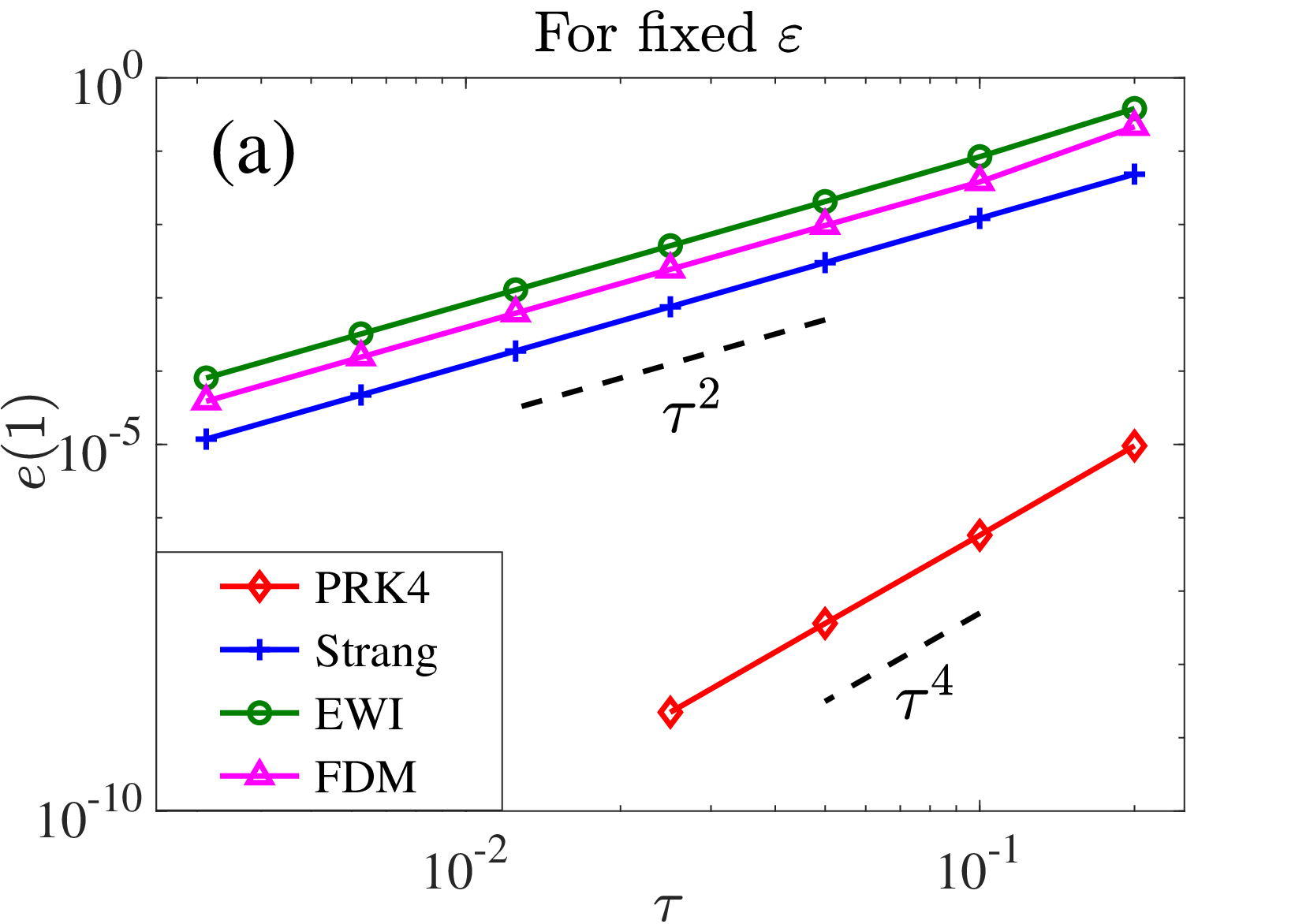
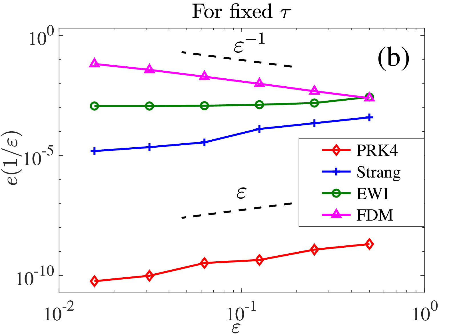
In this subsection, we compare the long-time temporal errors of the time-splitting methods with the finite difference method (FDM) and the exponential wave integrator (EWI) method[18, 19]. In order to compare the temporal errors, we adopt the Fourier pseudospectral method in space combined with each temporal discretization and choose a fine mesh size such that the spatial errors are neglected.
Refer to caption

Refer to caption

Figure 6: Temporal convergence rates of different temporal discretizations for the Dirac equation (4) over long-time dynamics at t=1/εt=1/\varepsilon: convergence rates in τ\tau (a), and convergence rates in ε\varepsilon (b).

Fig. 6(a) displays the temporal errors for the fixed ε=1\varepsilon=1 with different time step τ\tau. For the three second-order schemes, the second-order (Strang) time-splitting method obtains smaller temporal errors than the other two methods with the same time step. The fourth-order time-splitting method (PRK4) not only has higher order convergent rate but also gives much smaller errors than the other three methods with the same time step. Fig. 6(b) shows the long-time temporal errors of these methods for different ε\varepsilon with with a fixed time step τ\tau. The splitting methods have improved uniform error bounds like O⁡(ε​τ2)O(\varepsilon\tau^{2}) up to the long-time at O⁡(1/ε)O(1/\varepsilon). The EWI method has uniform error bounds, while the long-time temporal errors of the finite difference method depend on the parameter ε\varepsilon and behave like O⁡(1/ε)O(1/\varepsilon). As a result, time-splitting methods perform much better than FDM and EWI in the long-time simulations.

6 Conclusions

Improved uniform error bounds for the time-splitting methods for the long-time dynamics of the Dirac equation with small electromagnetic potentials were rigorously established. With the help of the unitary property of the solution flow in L2​(Ω)L^{2}(\Omega), the linear growth of the uniform error bound for the time-splitting methods was strictly proven. By employing the regularity compensation oscillation (RCO) technique, the improved uniform error bounds were proved to be O⁡(ε​τ2)O(\varepsilon\tau^{2}) and O⁡(hm+ε​τ2)O(h^{m}+\varepsilon\tau^{2}) up to the long-time at O⁡(1/ε)O(1/\varepsilon) for the semi-discretization and full-discretization, respectively. Numerical results were shown to validate our error bounds and to demonstrate that they are sharp. Finally, comparisons of different time discretizations were presented to illustrate the superior property of the time-splitting methods for the numerical simulation of the long-time dynamics of the Dirac equation.

Acknowledgment

This work was partially supported by the Ministry of Education of Singapore grant MOE2019-T2-1-063 (R-146-000-296-112, W. Bao & Y. Feng).

References

  • [1] W. Bao and Y. Cai, Mathematical theory and numerical methods for Bose-Einstein condensation, Kinet. Relat. Mod. 6 (2013) 1–135.
  • [2] W. Bao, Y. Cai and Y. Feng, Improved uniform error bounds for the time-splitting methods for the long-time dynamics of the Schrödinger/nonlinear Schrödinger equation, arXiv: 2109.08940.
  • [3] W. Bao, Y. Cai and Y. Feng, Improved uniform error bounds on time-splitting methods for long-time dynamics of the nonlinear Klein–Gordon equation with weak nonlinearity, arXiv: 2109.14902.
  • [4] W. Bao, Y. Cai, X. Jia and Q. Tang, Numerical methods and comparison for the Dirac equation in the nonrelativistic limit regime, J. Sci. Comput. 71 (2017) 1094–1134.
  • [5] W. Bao, Y. Cai, X. Jia and J. Yin, Error estimates of numerical methods for the nonlinear Dirac equation in the nonrelativistic limit regime, Sci. China Math. 59 (2016) 1461–1494.
  • [6] W. Bao, Y. Cai and J. Yin, Super-resolution of time-splitting methods for the Dirac equation in the nonrelativistic regime, Math. Comp. 89 (2020) 2141–2173.
  • [7] W. Bao, Y. Cai and J. Yin, Uniform error bounds of time-splitting methods for the nonlinear Dirac equation in the nonrelativistic limit regime, SIAM J. Numer. Anal. 59 (2021) 1040–1066.
  • [8] W. Bao and J. Yin, A fourth-order compact time-splitting Fourier pseudospectral method for the Dirac equation, Res. Math. Sci. 6 (2019) article 11.
  • [9] S. Blanes and P. C. Moan, Pratical symplectic partitioned Runge–Kutta and Runge–Kutta–Nyström methods, J. Comput. Appl. Math. 142 (2002) 313–330.
  • [10] J. W. Braun, Q. Su and R. Grobe, Numerical approach to solve the time-dependent Dirac equation, Phys. Rev. A 59 (1999) 604–612.
  • [11] W. Chen, X. Li and D. Liang, Energy-conserved splitting FDTD methods for Maxwell’s equations, Numer. Math. 108 (2008) 445–485.
  • [12] W. Chen, X. Li and D. Liang, Energy-conserved splitting finite-difference time-domain methods for Maxwell’s equations in three dimensions, SIAM J. Numer. Anal. 48 (2010) 1530–1554.
  • [13] P. A. M. Dirac, The quantum theory of the electron, Proc. R. Soc. Lond. A 117 (1928) 610–624.
  • [14] P. A. M. Dirac, Principles of Quantum Mechanics (Oxford University Press, 1958).
  • [15] G. Dujardin and E. Faou, Long time behavior of splitting methods applied to the linear Schrödinger equation, C. R. Acad. Sci. Paris 344 (2007) 89–92.
  • [16] G. Dujardin and E. Faou, Normal form and long time analysis of splitting schemes for the linear Schrödinger equation with small potential, Numer. Math. 108 (2007) 223–262.
  • [17] M. Esteban and E. Séré, Existence and multiplicity of solutions for linear and nonlinear Dirac problems, Partial Differ. Equ. Appl. 12 (1997) 107–112.
  • [18] Y. Feng and J. Yin, Spatial resolution of different discretizations over long-time for the Dirac equation with small potentials, arXiv: 2105.10468.
  • [19] Y. Feng, Z. Xu, and J. Yin, Uniform error bounds of exponential wave integrator methods for the long-time dynamics of the Dirac equation with small potentials, Appl. Numer. Math. 172 (2022) 50–66.
  • [20] F. Fillion-Gourdeau, E. Lorin and A. D. Bandrauk, Numerical solution of the time-dependent Dirac equation in coordinate space without fermion-doubling, Comput. Phys. Commun. 183 (2012) 1403–1415.
  • [21] L. Gauckler and C. Lubich, Splitting integrators for nonlinear Schrödinger equations over long times, Found. Comput. Math. 10 (2010) 275–302.
  • [22] F. Gesztesy, H. Grosse and B. Thaller, A rigorous approach to relativistic corrections of bound state energies for spin-1/2 particles, Ann. Inst. Henri Poincaré Phys. Theor. 40 (1984) 159–174.
  • [23] L. Gosse, A well-balanced and asymptotic-preserving scheme for the one-dimensional linear Dirac equation, BIT 55 (2015) 433–458.
  • [24] L. Gross, The Cauchy problem for the coupled Maxwell and Dirac equations, Commun. Pure Appl. Math. 19 (1966) 1–15.
  • [25] B.-Y. Guo, J. Shen and C.-L. Xu, Spectral and pseudospectral approximations using Hermite functions: Application to the Dirac equation, Adv. Comput. Math. 19 (2003) 35–55.
  • [26] E. Hairer, C. Lubich and G. Wanner, Geometric Numerical Integration: Structure-Preserving Algorithms for Ordinary Differential Equations (Springer-Verlag, 2002).
  • [27] C. Lubich, On splitting methods for Schrödinger-Poisson and cubic nonlinear Schrödinger equations, Math. Comp. 77 (2008) 2141–2153.
  • [28] Y. Ma and J. Yin, Error bounds of the finite difference time domain methods for the Dirac equation in the semiclassical regime, J. Sci. Comput. 81 (2019) 1801–1822.
  • [29] R. I. McLachlan and G. R. W. Quispel, Splitting methods, Acta Numer. 11 (2002) 341–434.
  • [30] G. R. Mocken and C. H. Keitel, Quantum dynamics of relativistic electrons, J. Comput. Phys. 199 (2004) 558-588.
  • [31] J. Shen, T. Tang and L.-L. Wang, Spectral Methods: Algorithms, Analysis and Applications (Springer-Verlag, 2011).
  • [32] G. Strang, On the construction and comparison of difference schemes, SIAM J. Numer. Anal. 5 (1968) 506–517.
  • [33] B. Thaller, The Dirac Equation (Springer-Verlag, 1992).
  • [34] H. F. Trotter, On the product of semi-groups of operators, Proc. Amer. Math. Soc. 10 (1959) 545–551.
  • [35] J. Yin, A fourth-order compact time-splitting method for the Dirac equation with time-dependent potentials, J. Comput. Phys. 430 (2021) 110109.