Kantorovich-Rubinstein distance and barycenter for finitely supported measures: Foundations and Algorithms
Abstract
The purpose of this paper is to provide a systematic discussion of a generalized barycenter based on a variant of unbalanced optimal transport (UOT) that defines a distance between general non-negative, finitely supported measures by allowing for mass creation and destruction modeled by some cost parameter. They are denoted as Kantorovich-Rubinstein (KR) barycenter and distance. In particular, we detail the influence of the cost parameter to structural properties of the KR barycenter and the KR distance. For the latter we highlight a closed form solution on ultra-metric trees. The support of such KR barycenters of finitely supported measures turns out to be finite in general and its structure to be explicitly specified by the support of the input measures. Additionally, we prove the existence of sparse KR barycenters and discuss potential computational approaches. The performance of the KR barycenter is compared to the OT barycenter on a multitude of synthetic datasets. We also consider barycenters based on the recently introduced Gaussian Hellinger-Kantorovich and Wasserstein-Fisher-Rao distances.
1 Introduction
Over the past decade, optimal transport (OT) based concepts for data analysis (Rachev and Rüschendorf 1998; Villani 2008; Santambrogio 2015, for a thorough treatment of the mathematical foundations of optimal transport see e.g.) have seen increasing popularity. This is mainly due to the fact that OT based methods respect important features of the data’s geometric structure. Furthermore, noteworthy advances have been achieved in various areas, such as optimisation (Bertsimas and Tsitsiklis 1997; Wolsey and Nemhauser 1999; Grötschel et al. 2012), machine learning (Frogner et al. 2015; Peyré et al. 2019; Xie et al. 2020), computer vision (Gangbo and McCann 2000; Su et al. 2015; Solomon et al. 2015) and statistical inference (Sommerfeld and Munk 2018; Panaretos and Zemel 2020; Hallin et al. 2021), among others. This methodological and computational progress recently also paved the way to novel areas of applications including genetics (Evans and Matsen 2012; Schiebinger et al. 2019) and cell biology (Gellert et al. 2019; Klatt et al. 2020; Tameling et al. 2021; Wang and Yuan 2021), to cite but a few. Of particular importance from a data analysis point of view are extensions to compare more than two measures, a prominent proposal being the Fréchet mean (Fréchet 1948), in the present context known as Wasserstein barycenter (Agueh and Carlier 2011). Wasserstein barycenters allow for a notion of average on the space of probability measures, which is well-adapted to the geometry of the data (Álvarez-Esteban et al. 2016; Anderes et al. 2016). With recent progress on their computation (Cuturi and Doucet 2014; Carlier et al. 2015; Bonneel et al. 2015; Kroshnin et al. 2019; Ge et al. 2019; Heinemann et al. 2022) they establish themselves even further as a promising tool in many fields of data analysis, such as texture mixing (Rabin et al. 2011), distributional clustering (Ye et al. 2017), histogram regression (Bonneel et al. 2016), domain adaptation (Montesuma and Mboula 2021) and unsupervised learning (Schmitz et al. 2018), among others.
However, a well known drawback of the Wasserstein distance and its barycenters in various applications is their limitation to measures with equal total mass. In fact, in many real world instances the difference in total mass intensity is of crucial importance. Employing vanilla Wasserstein based tools on general positive measures necessitates the usage of a normalisation procedure to enforce mass equality between the measures. This approach is, by design, oblivious to the mass differences between the original measures and can limit its use in applications. Exemplary, we mention that normalisation destroys stoichiometric features in the analysis of protein interaction and pathways as pointed out in Tameling et al. 2021. Overall, this might lead to incorrect conclusions on specific applications. An illustrative example is given in Figure 1.
1.1 Prior Work
The limitation of OT based concepts dealing only with measures of equal total mass has opened a wealth of approaches to account for more general measures. As an early proposal of this idea, the partial OT formulation (Caffarelli and McCann 2010; Figalli 2010) suggests to fix the total mass of the OT plan in advance, while relaxing the marginal constraints. Comparably more recent are entropy transport formulations11
1
Critically, this is not be confused with entropy regularized optimal transport, which is a popular computational approach adding an entropy penalty term to the OT problem to allow for efficient, approximate computations (Cuturi 2013; Benamou et al. 2015; Carlier et al. 2017). This general framework removes the marginal constraints and instead uses a divergence functional to measure the deviation between the transport marginals and the input measures. The entropy transport framework encompasses the Hellinger-Kantorovich distance (Liero et al. 2018; Chizat et al. 2018b), also known as Wasserstein-Fisher-Rao distance (Chizat et al. 2018a) and the Gaussian Hellinger-Kantorovich distance (Liero et al. 2018). Inherent to all of these models is their dependency on parameters whose exact influence on the models’ properties is generally not well understood. An alternative idea is based on extending the well-studied dynamic formulation of OT (Benamou and Brenier 2000) to measures with different total masses. With a focus on its geodesic properties, this approach has been studied in several works (Chizat et al. 2018a; Chizat et al. 2018c; Gangbo et al. 2019).
In this paper, we rely on a simple and intuitive idea based on the seminal work of Kantorovich and Rubinstein 1958. This accounts for mass construction and deletion at a cost modeled by some prespecified parameter (Hanin 1992; Guittet 2002, for details see also). It leads to the Kantorovich-Rubinstein distance (KRD) which curiously has been revisited several times under different names by various authors. For , it has been referred to as Earth Mover’s Distance (Pele and Werman 2008), and generalized Wasserstein distance (Piccoli and Rossi 2014), while for general common terminology includes Kantorovich distance (Gramfort et al. 2015), generalized KRD (Sato et al. 2020), transport-transform metric (Müller et al. 2020) and robust optimal transport distance (Mukherjee et al. 2021).
1.2 Contributions
In this work, we define barycenters with respect to the KRD and investigate their fundamental properties from a data analysis point of view. This extends the popular notion of Wasserstein barycenters to unbalanced barycenters (UBCs), i.e., barycenters of measures of different total masses. Similary, UBCs have been considered explicitly for the Hellinger-Kantorovich distance (Chung and Phung 2020; Friesecke et al. 2021) and for the partial OT distance for absolutely continuous measures (Kitagawa and Pass 2015). Notably, the well-known approach of matrix scaling algorithms has been shown to provide a general framework to approximate any UBC based on entropy optimal transport (Chizat et al. 2018b) of finitely supported measures. Closely related to our approach is the work by Müller et al. 2020 approximating the KR barycenter in the special case of point patterns.
The KR distance: Let be a finite metric space, where and
is the set of non-negative measures22 2 A non-negative measure on a finite space is uniquely characterized by the values it assigns to each singleton . To ease notation we write instead of . The corresponding -field is always to be understood as the powerset of . on . For a measure its total mass is defined as and the subset of non-negative measures with total mass equal to one is the set of probability measures . If is a measure on the product space its marginals are defined as and , respectively. For two measures we define the set of non-negative sub-couplings as
| (1) | ||||
Similarly, we denote the set of couplings between and as , where the inequality constraints in (1) are replaced by equalities. For and a parameter , unbalanced optimal transport (UOT) between two measures is defined as
| (2) | ||||

Notably, is finite for all measures with possibly different total masses and a solution of (2) always exists. Here, the parameter penalizes deviation of mass from the marginals of with respect to the input measures . In particular and unlike the (balanced) OT problem
defined only for measures with equal total mass , UOT in (2) relaxes the marginal constraint and allows optimal solutions to have more flexible marginals. Based upon UOT we define the -th order Kantorovich-Rubinstein distance between two measures as
| (3) |
For any , it defines a distance on the space of non-negative measures and it is an extension of the well-known -Wasserstein distance defined only for measures of equal total mass. Indeed, the KRD is shown to interpolate in-between OT on small scales and point-wise comparisons on large scales (Theorem 2.2) relative to the parameter . This allows for an intuitive interpretation of the KRD. More precisely, in Lemma 2.1, we detail a clear geometrical connection between the value of and the structure of the UOT. In particular, this contrasts the closely related partial OT problem (Figalli 2010) mentioned above. Employing Lagrange multipliers one can see that for any choice of , there exists a fixed mass of the partial OT problem, such that these two problems are equivalent. However, finding this value of requires to solve the UOT problem. We stress that the influence of on the resulting transport is in general hard to determine, while the impact of is intuitively clear. Thus, this perspective seems better suited to many applications.
For the specific case of measures supported on ultrametric trees (Section 2.1.1) we prove (Theorem 2.3) an analogue of the well-known closed formula for the -Wasserstein distance (Kloeckner 2015). Additionally, the computation of the KRD is known to be equivalent to solving a related balanced OT problem (Guittet 2002), allowing to apply any state-of-the-art solver with minimal modifications to compute the KRD and plan.
The KR barycenter: The KRD also lends itself to define a notion of a barycenter for a collection of measures as a generalization of the -Wasserstein barycenter defined for probability measures as
| (4) |
Here, is assumed to be embedded in some ambient space , e.g., an Euclidean space with . The distance on is understood to be the distance on restricted to . For , any measure
| (5) |
is said to be a -Kantorovich-Rubinstein barycenter or -barycenter for short33
3
For the sake of readability, the weights in this definition are fixed to , though it is easy to adapt all instances of their occurrence in this work to arbitrary positive weights , summing to .. We refer to the objective functional as (unbalanced) -Fréchet functional.
Notably, -barycenters’ support is not restricted to the finite space which raises fundamental questions on its structural properties. In the following, we establish that there exists a finite set containing the support of any -barycenter (Section 2.2). Indeed, this set can be explicitly constructed from the support of the individual ’s, but its size grows exponentially in the number of individual measures. However, we prove that there always exists a sparse -barycenter whose support size is at most linear in the number of measures (Theorem 2.5). We note that these properties are analogs of well-known properties of Wasserstein barycenters (Anderes et al. 2016), that we re-establish for the unbalanced setting.
Comparably, employing more general entropy transport distances, we are not aware of any similar structural description of their barycenters in terms of the input measures and the parameter. Notably, the entropy optimal transport barycenter of dirac measures is not necessarily finitely supported itself (Friesecke et al. 2021, for an example see). In contrast, our explicit structural description of the support of KR barycenters provides an immediate understanding of its properties for a given choice of . This clear link between and the -barycenter also allows to incorporate previous knowledge of the measures or the ground space into the choice . The -barycenter can be tuned to be more flexible and provide superior performance compared to its -Wasserstein counterpart by avoiding to normalise each measure. An illustrative example is included in Figure 2, where the -barycenter detects all clusters correctly, while the Wasserstein barycenter does not provide any structural information on the underlying measures. This showcases potentially superior robustness and flexibility of the -barycenter compared to the Wasserstein barycenter. We study this comparison in more detail on multiple synthetic data sets in Section 4. Here, the computational results44
4
An implementation can be found in the R package WSGeometry on CRAN. are based on the fact that, due to our structural analysis of the support of the -barycenter, it is straightforward to modify any given state-of-the-art solver for the Wasserstein barycenter problem to solve the -barycenter problem (Section 4.1).
2 Kantorovich-Rubinstein Distance and -Barycenter
In this section, we provide some theoretical analysis of the structural properties inherent in the UOT in (2) and as a consequence to the KRD in (3). We also focus on the variational formulation defining the -barycenter in (5).
2.1 KR Distance
In this subsection, we focus on structural properties of minimizers for UOT in (2) and their consequences for the KRD. Notably, one can equivalently restate the penalization of total mass in (2) as
| (6) |
While in (2) the parameter controls the deviation of the total mass of , the alternative representation (6) demonstrates its marginal characterization. Indeed, the parameter specifies the maximal distance (scale) for which transportation is cheaper than creation or destruction of mass. More precisely, each optimal solution for (2) induces a directed transportation graph between the support points of (source points) and the support points of (sink points). By definition, the graph contains a directed edge if and only if . For a directed path in its path length is defined as . The parameter determines the maximal path length for any path in as the following statement demonstrates.
Lemma 2.1.
A proof is included in Section A.2. Lemma 2.1 shows that the underlying transportation graph has maximal path length which limits the interaction between source and sink points. It will be of crucial importance for closed formulas on ultra-metric trees in the following subsection. As an immediate consequence we obtain some important statements on the KRD in (3) along with its metric property.
Theorem 2.2.
For any and parameter the following statements hold:
- (i)
The -th order KRD in (3) defines a metric on the space of non-negative measures .
- (ii)
If , then it holds that
where is the total variation distance. The same equality holds for all if for all or if for all .
- (iii)
If and , then it holds that
- (iv)
If , then it holds
We stress that the metric property of the KRD in Theorem 2.2 (i) has already been established in specific instances, e.g., for (Piccoli and Rossi 2014). Our proof follows that of Theorem in Müller et al. 2020 for uniform measures on point patterns with minor modifications.
Theorem 2.2 demonstrates how two measures are compared with respect to KRD. Depending on the parameter the optimal value interpolates between -th order Wasserstein distance on small scales and total variation on larger scales with respect to .
Equivalently, these properties can be shown by considerations of the dual program for UOT in (2) given by
| () | ||||
where the equality holds due to strong duality. For this can be further specified to
which reveals its relation to the flat metric (Bogachev 2007) as observed in Lellmann et al. 2014; Schmitzer and Wirth 2019. As in general , the bound on dual feasible solutions is necessary for the dual to be finite. However, if the measures have equal total mass and , then the bound on dual feasible solutions is redundant and we obtain the dual of the usual OT problem
| () | ||||
2.1.1 KR Distance on Ultrametric Trees
For OT, the approximations of the underlying distance by a tree metric are common tools for theoretical and practical purposes. The former is usually employed for rates of convergence for the expectation of empirical OT costs (Sommerfeld et al. 2019) while in the latter tree approximations serve to reduce the computational complexity inherent in OT (Le et al. 2019). OT on ultramatric trees is also applied for the analysis of phylogenetic trees (Gavryushkin and Drummond 2016). For an efficient computational implementation of UOT on tree metrics we refer to Sato et al. 2020. Notably, while OT with tree metric costs has a closed form solution, this fails to hold for its UOT counterpart. An exception is given in terms of ultrametric trees for which not only OT (Kloeckner 2015) but also UOT admits a closed form solution, which we establish in this subsection.
To this end, consider a tree with nodes , edges attached with (non-negative) weights for and a designated root r. Two nodes are connected by a unique path denoted either represented by a sequence of nodes or as a sequence of edges. The distance is equal to the sum of the weights of those edges contained in . A leaf of is any node such that its degree (number of edges attached to the node) is equal to one and the set of all leaf nodes is denoted as . A node is termed parent of node v denoted by if both are connected by a single edge but is closer to the root than v. The parent of the root node is set to . For a node v its children are the elements of the set . Notice that with this definition v is a child of itself (Figure 3 (a) for an illustration).
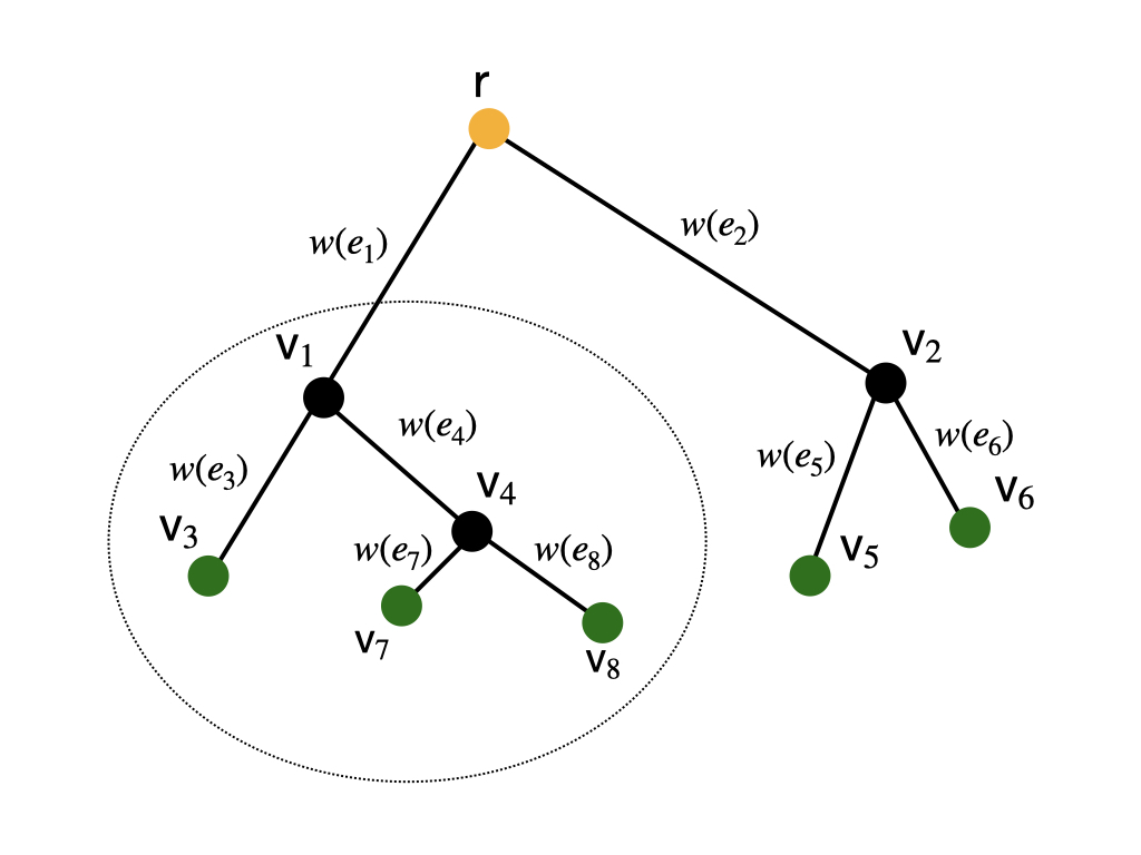
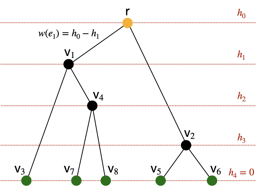
A tree is termed ultrametric tree if all its leaf nodes are at the same distance to the root. Equivalently, there exists a height function that is monotonically decreasing meaning that and such that for . The distance is set to and extended on the full tree (Figure 3 (b) for an illustration).
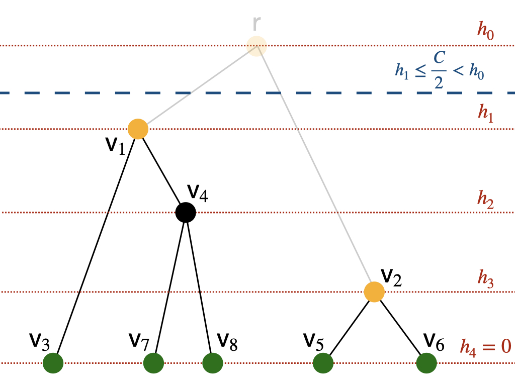
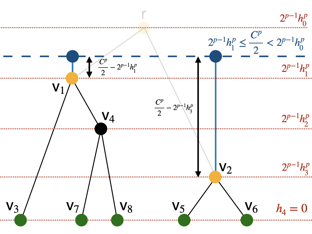
Consider an ultrametric tree with height function and measures supported on the leaf nodes . We prove that the -th order KRD admits a closed formula for such a setting. Intuitively, the parameter restricts transportation of mass up to a certain threshold allowing to decompose into subtrees. Mass transportation is restricted solely within each subtree whereas mass abundance or deficiency is penalized with parameter for each particular subtree (Figure 4 for an illustration). We define the set
| (7) |
with the convention that if and for a node set
Theorem 2.3 (KR on ultrametric trees).
Consider an ultrametric tree with leaf nodes and height function inducing the tree metric . For any and two measures supported on the leaf nodes of it holds that
The closed formula in Theorem 2.3 decomposes the underlying UOT into two tasks. While summing over subtrees carried out by the outer sum, the inner sum consists of two terms. The first considers OT within each subtree whereas the second accounts for mass deviation on that particular subtree.
The proof of this formula is given in Section A.2.1.
2.2 -Barycenters

In the finite setting considered in this work a -barycenter as defined in (5) always exists, but is not necessarily unique. Moreover, the location and structure of the support of the -barycenter are not fixed and hence unknown. For the Wasserstein barycenter there exists a finitely supported, sparse barycenter in this context (Anderes et al. 2016; Le Gouic and Loubes 2017). We establish analog properties of the -barycenter.
Definition 2.4.
Let be a metric space, and . A Borel barycenter application associates to any points a minimum of , i.e.,
A Borel barycenter application is in general not a function since the minimum does not need to be unique. In particular, only means that is one of the minima of the average distance function. As the measures are defined on we usually restrict the Borel barycenter application to inputs from the space . We define the full centroid set of the measures as
| (8) | ||||
and the restricted centroid set
| (9) | ||||
We stress that for each -tupel one fixed representative of is chosen for the construction of the centroid set . To streamline the presentation any statement concerning in the following theorem is to be understood in the sense that there exists a choice of such that the statement holds true.
Theorem 2.5.
Let be a collection of non-negative measures on the finite discrete space . For any it holds that
- (i)
Moreover, any -barycenter satisfies and its total mass is bounded by
- (ii)
For any -barycenter and any point , there exist UOT plans between and for , respectively, such that if , then there exists , for , and for with , if .
Additionally, if for any it holds that(10) then for .
- (iii)
If for then there exists a -barycenter such that
- (iv)
If , then it holds
- (v)
Furthermore, set and define
If , then the -barycenter is given by
- (vi)
Let and let be ordered such that for . Suppose that is odd or there there exists no point contained in at least different support sets. Then, for any -barycenter it holds that . Else, there exists at least one -barycenter with this total mass.
The proof is based on the fact that finding a -barycenter can be proven to be equivalent to solving a multi-marginal optimal transport problem (Section 3.2). Statement provides insights into the structure of the support of any -barycenter and its dependency with respect to the magnitude of . The definition of can be understood as a joint restriction on combined with an individual restriction on each of the original centroid points of . The joint restriction ensures that simply deleting any mass at a given centroid point (and thus reducing the total mass of the measure) does not improve the objective value. This is a minimal feasibility assumption on the considered centroid point, as otherwise no measure containing this point can be optimal. The second restriction concerns each point individually. If a point has a distance larger than from a point , then, by Lemma 2.1, there is no transport between and . Thus, centroids which have have a larger distance to one of the points they are constructed from can not be in the support of any -barycenter. This also gives rise to some helpful intuition for the support structure of any -barycenter. Considering all -neighbourhoods around any of the support points of the , then a -barycenter can only have support in regions where at least balls from different measures intersect. A visual representation of this is given in the center of bottom row of Figure 5. By definition, the sets are equipped with a natural ordering in the sense that if then . Moreover, if is large enough then . We illustrate these sets in the top row Figure 5. We observe that the cardinality of the restricted centroid set in (9) decreases with decreasing . In the extremes for large the restricted centroid sets coincides with the full centroid sets in (8) that is independent of . For small , if there is no point which is contained in the support of at least measures, the restricted centroid set is empty. For an illustration we refer to the top row of Figure 5.
Property is an analogue to a well-known characterization (Anderes et al. 2016) of the -Wasserstein barycenter on with Euclidean distance , where the transport from the barycenter to the underlying measures is characterized by a transport map. The corresponding statement for the -barycenter holds true as well in this context. Indeed, on condition (10), which can be understood as an injectivity-type assumption on the barycentric application, is satisfied due to the fact that . However, for this assertion does not hold. Consider and measures , then any measure of the form for any is a -barycenter for . Thus, there only exist mass-splitting UOT plans between and and the transport is not characterized by a transport map. On more general spaces such as a tree rooted at , three leaves and positive edge weights the barycenter on of any two leafs , is the root . In particular, in this example, or in fact in any tree which has a vertex with degree of at least three55
5
The degree of a vertex in a graph is the number of vertices which are adjacent to it. condition (10) fails. The unique -barycenter of two measures and is given by . Thus, there are again only mass-splitting UOT plans between and and . However, for the unit circle equipped with its natural arc-length distance property (10) does hold. Assume , and for each denote and as the halfcircle right and left of , respectively. It is straightforward to see by contraposition that if it holds , then this implies and . However, it also holds , and thus . In particular, this implies that either and or vice versa and hence . The case is analog and the case clear.
Property guarantees the existence of sparse -barycenters. For large the size scales as , growing essentially exponentially in . However, here we see that there always exists a -barycenter supported on a sparse subset of which has cardinality growing only linearly in . Part simply extends the montonicity of the -KRD to the -Fréchet functional. Statement yields a critical point after which decreasing does no longer change the resulting -barycenter and provides a closed form characterisation of the -barycenter in this context. Finally, statement enables control on the total mass of the -barycenter for large values of . In particular, since the total mass is close to the median of the total masses of the , we point out that the total mass of the -barycenter in this setting is robust against outliers. A small amount of measures with unreasonably high mass has no impact on the total mass of the -barycenter.
Naturally, we compare the -barycenter to its popular Wasserstein analogue in (4). As proven in Le Gouic and Loubes 2017 (Anderes et al. 2016, and initially for for by) the support of any -Wasserstein barycenter is contained in
| (11) |
Compared to the -Wasserstein barycenter of the probability measures the restricted centroid set allows more flexibility for specific cases and can provide a more reasonable representation of the data. We illustrate this in Figure 5 (bottom-left/right) where the -barycenter clearly represents all clusters while the -Wasserstein barycenter fails to capture them. Nevertheless, if is large enough and all measures have equal total mass both barycenters coincide.
Corollary 2.6.
If and , then any -Wasserstein barycenter is also a -barycenter and vice versa.
While this shows that the -barycenter is a strict generalisation of the usual -Wasserstein barycenter as the solutions coincide for large , for smaller values of there can be significant differences. One such striking difference between the -Wasserstein barycenter and the -barycenter comes in the form of a localization property. Let such that with for all and for all . Here, the barycenter tends to place mass between the clusters . However, a -barycenter is obtained by combining barycenters of the measures restricted to the , respectively.
Lemma 2.7.
Let such that for all it holds for some with for all and for all . For , let
where is the convex hull of for . Then, the measure is a -barycenter of .
3 A Lift to Optimal Transport, Wasserstein Barycenters and Multi-Marginal Optimal Transport
In this section, we provide the necessary tools and framework to establish our results in the previous section. Following the ideas of Guittet 2002 we state UOT in (2) as an equivalent balanced OT problem. We extend this idea to the -barycenter, showing it to be equivalent to a specific Wasserstein barycenter problem as well as a balanced multi-marginal optimal transport problem.
3.1 A Lift to Optimal Transport
We fix a parameter , introduce an additional dummy point and define the augmented space with metric cost
| (12) |
Notably, defines a metric on (Müller et al. 2020, Lemma A1). Consider the subset of non-negative measures whose total mass is bounded by . Setting , any measure defines an augmented measure on such that . Hence, for two measures we can define the OT problem on between their augmented measures . In fact, it holds that
where the first equality follows by Lemma 2.1 as for any optimal solution it holds if and the second follows by (Guittet 2002, Lemma 3.1). The same equalities remain valid replacing by an arbitrarily large constant as summarized by the following lemma.
Lemma 3.1.
Consider with extended versions . Then for any it holds that
Proof.
For , the result is trivial since by duality only depends on the difference of the measures. For we invoke -cyclical monotonicity (Villani 2008, Thm. 5.10) of any OT plan and use the property that . This yields that which leads to the desired conclusion. ∎
3.2 A Lift to Wasserstein Barycenters
We can also lift the optimization problem defining a -barycenter to an equivalent -Wasserstein barycenter formulation (4). Augmentation of the underlying measures, however, is not straightforward as the total mass of the -barycenter is unknown. A first crude upper bound on its total mass leads to a feasible approach.
Lemma 3.2.
Consider and let be their associated unbalanced Fréchet functional. Then it holds that
More precisely, any -barycenter of satisfies .
Proof.
Assume first that there exists a measure such that where no transport between and any occurs in the optimal solution of for and it holds . Thus it holds
and we improve the objective value of by removing . Hence, let be any measure such that . Consider the optimal solution for for each . Decompose the measure , where is the mass of transported to according to and which is not yet included in any for . Clearly, and we conclude that
By our first considerations the claim follows. ∎
Given the upper bound on the total mass of any -barycenter at our disposal we can formulate a lift of the -barycenter problem to a related -Wasserstein barycenter problem. For this, let endowed with the metric in (12) (replace by and recall that ) and augment the measures to where for . In particular, and we can define the augmented -Fréchet functional
where by definition is restricted to measures with mass .
Lemma 3.3.
For consider measures and their augmented versions , respectively. Then it holds that
for all such that and in particular
The proof of this Lemma is given in Section A.1.
Remark 3.4 (Optimal -barycenters).
Lemma 3.3 states that the optimal objective value for the -barycenter is equal the related -Wasserstein barycenter problem on the augmented space. In particular, the proof also reveals that if is a -Wasserstein barycenter for the augmented measures then is a -barycenter for the measures . Vice versa, if is a -barycenter for the measures then is a -Wasserstein barycenter for the augmented measures .
3.3 A Lift to Multi-Marginal Optimal Transport
On the augmented space equipped with metric in (12), we define for and a Borel barycenter application that takes as input and outputs any minimizer of the function
Of particular interest to us is the barycentric application restricted to inputs from . However, we collect some of its key properties for general input . For this, we define the index set
If clear from the context, then the dependence on is suppressed and the set is simply denoted as .
Lemma 3.5.
Fix some parameter and consider the space with metric as defined in (12). For points it holds that
- (i)
if and only if for any . In particular, if strict inequality holds then is unique.
- (ii)
If then it holds with uniqueness if .
- (iii)
If then it holds
- (iv)
If , then for any points with it holds that where the latter one is defined with respect to the usual metric on .
A proof of this result is provided in Section A.1. Lemma 3.5 allows to characterize the centroid sets of the augmented measures defined as
| (13) | ||||
Remark 3.6.
We point out that computing is in general a difficult optimisation problem. While for squared euclidean distance, computing the barycentric application simply amounts to taking the mean of the , even on the non-augmented space, there are no closed form solutions available for most choices of distances and values of . This problem is exacerbated by the truncation of the distance at (Müller et al. 2020, as also pointed out in), since it implies that disregarding a certain subset of points and just computing the barycenter with respect to the remaining might in fact be optimal. However, initially it is not clear which to choose, turning this into a difficult combinatorial problem.
Recall that for any measure its support is contained in a subset of . The augmented measure is extended by an additional support point at . In particular, while the centroid set is a subset of it only depends on the support of the measures contained in .
Corollary 3.7.
For the centroid sets of the augmented measures with it holds
Proof.
The first inclusion follows by statements (i) and (iii) in Lemma 3.5 and the observation that . The second by applying . ∎
Remark 3.8.
One could define in terms of instead of to obtain equality in the first inclusion. Replacing by in the definition of the centroid set would not alter any of the related proofs and yield slightly sharper control on the support of -barycenter. However, as we consider the given definition to be more intuitive, we omit this improvement in the statement of the theorem.
Let be the set of measures on whose -th marginal is equal to for all . We refer to the elements of this set as multi-couplings of . For define the augmented multi-marginal transport problem as
| (14) |
where
The relation between the augmented multi-marginal transport formulation (14) and the -barycenter is as follows.
Proposition 3.9.
Let and be their augmented counterparts. If is a solution to the augmented multi-marginal problem (14), then the measure is a -barycenter of the measures , where denotes the pushforward of under . Moreover, for every -barycenter , there exists a solution to the augmented multi-marginal transport problem, such that
In particular, it holds that
The proof follows straightforwardly along the lines of related statements for the multi-marginal optimal transport problem (Le Gouic and Loubes 2017, Theorem 8; Masarotto et al. 2019, Lemma 8 or Panaretos and Zemel 2020, Proposition 3.1.2). This correspondence between the -barycenter problem and a balanced multi-marginal optimal transport serves as one of the key components in the proof of Theorem 2.5.
4 Computational Issues and Numerical Experiments
We present approaches to compute the -barycenter problem by solving related OT problems. Based on this, we investigate the performance of the Wasserstein and -barycenters on multiple synthetic datasets. For reference, we also report on results for two related concepts of unbalanced barycenters (UBCs), namely the Gaussian-Hellinger-Kantorovich and Wasserstein-Fisher-Rao barycenter.
4.1 Algorithms
Theorem 2.5 and Proposition 3.9 both allow to pose the augmented problem (recall Section 3) as a linear program and using Lemma 3.3 one can obtain a solution to the original problem by solving the augmented one. Using any linear program solver this enables the direct computation of an exact solution of this problem. However, the number of variables in this approach scales as the size of and hence it turns out to be infeasible already for relatively small instance sizes. To compute -barycenters at larger scales we revisit iterative methods to solve the (balanced) Wasserstein barycenter problem and give instructions how to use modifications of them to compute -barycenters. In particular, we detail a multi-scale method which solves successive fixed-support -barycenter LPs on increasingly refined support sets. This provides a meta-framework to adjust state-of-the-art solvers for the Wasserstein barycenter for -barycenter computations.
To construct the augmented problem we add the dummy point to the support of the ’s, while setting its distance to all other locations to be . Note, that by Lemma 2.1 and Lemma 3.1 the truncation of at can be omitted if . If this is not the case, we can enforce it by adding additional mass at in all augmented measures without changing the optimal value.
4.1.1 LP-Formulation for the -Barycenter
Using property (i) from Theorem 2.5, we can rewrite the augmented -barycenter problem as a linear program similarly to the usual -Wasserstein barycenter problem (4). However, compared to the latter one, we replace the standard centroid set from (11), by the centroid set of the augmented measures from (13). This yields
where is the cardinality of the support of the augmented measure . Here, denotes the distance between the -th point of and the -th point in the support of , while is the vector of masses corresponding to . For practical purposes it may be advantageous to solve the multi-marginal problem instead of the -barycenter problem. This changes the number of variables from ) to and the number of constraints from to . Depending on the value of , and hence the cardinality of , it is possible to pick the problem with the smaller complexity.
While this formulation is appealing for proving theoretical statements as provided in Theorem 2.5, it quickly becomes computationally infeasible even for small scale problems as the number of variables in the LP grows potentially as . However, it still enables exact computations of -barycenters for small scale examples, which is currently impossible for general UBCs. Though, while there has been some recent advancement for the -Wasserstein barycenter in special cases (Altschuler and Boix-Adsera 2021) these LP-based algorithms ultimately do not scale to large instance sizes.
4.2 Iterative Algorithms and the Multi-Scale Approach

For the Wasserstein barycenter, iterative methods computing approximate barycenters, with a per iterations complexity only linear in the number of measures, enjoy great popularity. Most well known is the fixed-support Wasserstein barycenter (Ge et al. 2019; Lin et al. 2020; Xie et al. 2020) approach, aiming to find the best approximation of the barycenter on a pre-specified support set, for which a variety of methods is available. We utilise this fixed-support approach for the augmented -barycenter problem by adding the dummy point to the given support and constructing the cost as described above. This yields a meta-framework which allows to employ fixed-support Wasserstein barycenter algorithms for fixed-support -barycenter computation. One can also modify more general free support methods (Cuturi and Doucet 2014; Ge et al. 2019; Luise et al. 2019), which usually alternate between updating the support set of the barycenter and its weights on this set, to provide approximate -barycenters. However, the necessary position updates usually explicitly or implicitly rely on being able to compute the barycentric application efficiently. Recalling Remark 3.6, this is in general not tractable for the augmented problem, which severely hinders the use of these approaches. Thus, it is tempting to avoid these issues by approximating with a large finite space, i.e., by taking a grid of high-resolution, and solving the fixed support -barycenter problem on this set. However, solving the fixed-support problem on this large space requires significant computational effort. We advovate an alternative by adapting the ideas of multi-scale methods for the Wasserstein distance/barycenter (Mérigot 2011; Gerber and Maggioni 2017; Schmitzer 2019) to the -barycenter setting. The idea of this approach is to start with a coarse version of the problem and then successively solve refined problems, while using the knowledge of the coarse solution to reduce the complexity of the finer ones.
Thus, we initialise the support set of the barycenter as a fixed grid of size in . In the -th step of the algorithm, after solving the fixed-support problem, we remove the grid points which have zero mass and replace the remaining ones with its closest points in a refined version of the original grid of size . This can be understood as solving the fixed-support problem on successively finer grids, while incorporating information provided by having already solved a coarser solution of the problem. We terminate the method once a pre-specified resolution has been reached. This allows to obtain fixed-support approximation of the -barycenter on fine grids without having to optimise over the full support set.
We point out that this approach, while inspired by multi-scale approaches is more closely related to the formerly mentioned free-support methods. As such it does in general not yield a globally optimal fixed-support -barycenter at the finest resolution. Instead it converges to a local minimum of the unbalanced Fréchet functional depending on the resolution of the initial grid. This is a common problem among alternating procedures for the free-support barycenter problem and can be attributed to the fact that the Fréchet functional is non-convex in the support locations of the measures. However, we stress that with this approach we observe reasonable approximations of the -barycenter while avoiding the inherent problems of generalising usual position update procedures discussed above. In particular, we do not have to solve the barycenter problem at any point. Additionally, we note that the initial grid size should be chosen at least fine enough that the distance between two adjacent grid points is smaller than . Otherwise it is possible that support points lying between two grid points, having distance larger to both, are not accounted for. For a visual illustration of the algorithm we refer to Figure 6.
4.3 Synthetic Data Simulations
We test the performance of the -barycenter as a data analytic tool compared to the usual -Wasserstein barycenter on a multitude of datasets. We base our computations on the MAAIPM method (Ge et al. 2019), which allows for high-precision approximations of barycenters up to moderate data sizes. The algorithm has been deployed to solve the fixed-support -barycenter problems arising in the multi-scale method detailed above. For all experiments, the initial grid size as been set to and the refinement is terminated at a gridsize of . Values below have been considered as zero for the purposes of grid refinement. All experiments have been carried out on a single core of an Intel Core . Implementations of our used method and some alternatives can be found as part of the R-package WSGeometry (on CRAN).

Mismatched Shapes
This first set of examples mainly serves as starting point to illustrate improved performance of the -barycenter compared to the -Wasserstein barycenter. A prototypical benchmark for the -Wasserstein barycenter are two nested ellipses as popularized in Cuturi and Doucet 2014. For our example of nested ellipses, we assume that the support of each measure consists of nested ellipses, but the number of ellipses varies between the individual underlying measures. Specifically, we assume that for each the number of ellipses is uniformly random in and that each ellipse is discretised onto support points with unit mass, respectively. This can be seen in Figure 7. We observe that while the -Wasserstein barycenter recovers the elliptic shape of the underlying measures, it fails to produce distinct ellipses and instead produces something akin to a ring. In contrast, the -barycenter yields two distinct ellipses, which coincides with the expected number of ellipses in one of the measures. This aligns well with intuition that the -barycenter will simply disregard any additional structures which are not present in a sufficient amount of underlying measures. In contrast, the -Wasserstein barycenter does not allow for this flexibility which enforces additional support points.

Local Scale Cluster Detection
Recall the setting of Figure 2. In the following class of examples, we are interested in datasets which possesses a natural cluster structure. Let be convex, disjoint sets and assume that for all . If the diameter of all is bounded from above by and that the distance between each two is at least , then Lemma 2.7 guarentees that the -barycenter detects all of the clusters in which at least measures have positive mass. In particular, by Theorem 2.5 (v) the -barycenter will have mass in all of those clusters. Intuitively, this setting is reasonable if, for instance, it is already known that any interactions between support points of different measures are limited to scales below a certain threshold, which should then be chosen as . The lower bound on the inter-cluster distance ensures that any pair of two clusters is well-separated, ensuring that it is always possible to distinguish between two different clusters, as they can not be arbitrarily close to each other.
In Figure 2 the -Wasserstein barycenter completely fails to capture the geometric data structure. Most of its mass is between the clusters and the outer clusters have nearly no mass. Moreover, the elliptic structure within each cluster is clearly not captured. In contrast, the -barycenter not only captures all clusters, it also distinguishes between the difference in intensity (expected number of ellipses) in the clusters, matching the theoretical guarantees of Lemma 2.7. We stress that for this example the choice of is of particular importance. If we choose too large, the -barycenter will fail to recover the data’s support structure (for an illustration of the -barycenter in this example over a range of values of see Figure 8). Consequently, it is crucial to choose appropriately. In this example, the barycenter appears to be stable and detect all clusters for . Notably, if the locations of the clusters are already known, this setting also allows for parallel computations of the -barycenter, where the problems are solved separately on each cluster and recombined at the end (Lemma 2.7).
Randomly distorted Measures
In a statistical context it is important to investigate the stability of the -barycenter under random distortions. We fix a reference measure on and generate a set of measures by random modifications of . We then attempt to recover by computing the -Wasserstein and -barycenter of these measures, respectively.
In the following, let denote a Bernoulli random variable with mean , a Poisson distribution with mean and a uniform distribution on . We generate as follows:
For initialise , then succesively modify based on the four following steps.
- (i)
Point Deletion: Fix and . We draw a Ber( random variable. If it takes the value , then we draw and select points in the support of uniformly by drawing without replacement. These points (and their mass) are not contained in , since they have been deleted.
- (ii)
Point Addition: We fix parameters . Draw a Ber() random variable. If it takes the value , draw a Poi() random variable . Then, generate random variables following a normal distribution with mean and covariance matrix . Add these support points to , where the weight of each of these points is determined by independent random variables.
- (iii)
Position Change: Fix parameters with and . For each in the support of , we draw a random variable and shift the position of by it.
- (iv)
Weight Change: Fix parameters with . For each support point of with weight , we draw a random variable and change the weight of in to be .
An example of this setting can be seen in Figure 9. Comparing the two barycenters displayed there to the original measure reveals that, while the rough shape of the -Wasserstein barycenter is correct, its mass is spread out over a larger area and it has a significantly larger number of support points. Since all measures have been normalised, we have also lost all information on the mass of . Contrary to that, the -barycenter retrieves the original measures recovering the location and number of the of support points closely. Additionally, it also has a mass which only deviates from the original mass by about . If one is only interested in recovering the general shape of the data, both approaches provide comparable performance. However, if the measures total mass and more detailed support structure are of importance the -barycenter appears to be preferable.

Total Mass Intensity

While the -Wasserstein barycenter of probability measures has mass one, the mass of the -barycenter depends on as well as the geometry of the measures . Exact values for the mass of a -barycenter without detailed computations, are only available in the limiting scenarios where is extremely small or large relative to the other distances in . For the former, we know by Theorem 2.5 that the barycenter has mass zero for disjoint measures and for the latter, Theorem 2.5 yields that there exists a -barycenter with total mass intensity equal to the median of . For intermediate values of , Theorem 2.5 yields the upper bound by . To highlight some possible behaviours of the total mass intensity of -barycenter we consider three specific examples in Figure 10. We note that in all three cases at about the mass of the barycenters is at the median of their respective and does no longer change with increasing . This is significantly smaller than the requirement in Theorem 2.5 , which underlines the fact that while in the worst case, this lower bound is sharp, in many examples the total mass of the -barycenter stabilises significantly earlier. Moreover, none of the three curves is monotone. Instead the total mass of the barycenter is increasing up to a certain point, after which it decreases until it reaches the median of the masses. This makes intuitive sense, as the measures are disjoint, thus for small the barycenter is empty and starts to grow in mass quickly as the points within the clusters can be matched. In particular, the differences in intensity between clusters might lead to a total mass over the median , as by Lemma 2.7 the total mass intensity of the -barycenter is , where denote the respective cluster locations. For larger these clusters start to merge and support points between the clusters reduce the total mass. In particular, these points can be seen clearly in the plot. Up until about , which is the cluster size, the mass of the barycenters rises sharply, before stabilising until the intercluster distance is reached. This is about for the green and blue lines and about for the red line (since the measures in this example are generated by halving the intercluster distance from the green one). This behaviour highlights the sensitivity of the mass of the -barycenter to the geometry of the measures. It is therefore impossible to infer the total mass of the -barycenter from the magnitude of alone without accounting for the specific measures. However, analysing the structural properties of the support sets of the measures might provide a good indication at what values of changes in drastic behaviour of the total mass are to be expected.
4.4 Comparison with Related Unbalanced Barycenter Concepts
We compare the -barycenter with two alternative UBC approaches.
The Gaussian-Hellinger-Kantorovich Barycenter: This example falls in the general framework of optimal entropy transport problems. Measuring deviation between a feasible solution and the input marginals is carried out via the Kullback-Leibler divergence defined for 66
6
A measure is said to be absolutely continuous (denoted ) with respect to another measure if implies for any measurable set . as
If the value of is set to be . For a parameter , the Gaussian-Hellinger-Kantorovich Distance (Liero et al. 2018) is defined as
where and denote the respective marginals of . The barycenter is defined as
The Hellinger-Kantorovich Barycenter: The Hellinger-Kantorovich distance, also known as Wasserstein-Fisher-Rao distance (Liero et al. 2018; Chizat et al. 2018a), is closely related to the Gaussian-Hellinger-Kantorovich distance. For fixed parameter , referred to as the cut-locus, it is defined as
where . For a fixed cut-off locus , the barycenter is defined as
Comparing the barycenters: As the resulting barycenters vary significantly in all three cases, depending on the parameters , we compare their behaviour upon change of parameter.

As a simple example, we consider four measures supported on subsets of a grid on , displayed in Figure 11. To ensure fair comparison, we deploy the same method based on the general scaling method (Chizat et al. 2018b) to approximate the UBC in all three cases. However, we point out that this implies disregarding the ambient space and instead taking the minimum over all positive measures supported on a prespecified grid in .
For high parameter values all three approaches yield similar results. This is, of course, to be expected, since these distances interpolate between -Wasserstein distance and total variation/Kullback-Leibler distance and large parameters correspond to a setting being close to the Wasserstein distance. The KR barycenter has mass zero for small choice of by Theorem 2.5 (iv), since the four measures have disjoint support. After reaching a threshold of , the mass in the -barycenter starts to increase as mass is added in the center of the unit square until at the mass of an individual data measure is reached.
For small the barycenter has small mass and its support is close to that of a linear mean of the four measures, though the total mass intensity is significantly lower than for the original measures. With increasing the mass starts to increase and to smear into the middle of the unit square, until a large square, encompassing all four data supports, is formed. After this point increasing causes the square to contract while its mass increases. Finally, we approach a single square at roughly the same size as the squares in the underlying measures for large .
The barycenter is close to a linear mean of the four measures for small cut-off. Increasing initially reduces the mass at each of the square locations. At a threshold of , we observe a change, where part of the mass is moved vertically or horizontally to the mid points between the squares in a rectangular shape. Until all mass is shifted to these ”middle-rectangles”, at which point a second shift occurs, where the mass from these rectangles starts to move towards a square in the center. At , all mass has been shifted towards a square in the center and there is no further change in the HK barycenter, when increasing .


Additionally, we consider Figure 13, where the three unbalanced barycenter models are compared on three exemplary classes based on the MNIST dataset. Here, the original images have been rescaled to sizes between and and embedded in a random subgrid of a image. In this setting, there is a notable distinction between the GHK barycenter and the KR and HK barycenters. While for the former, the overall shape is recovered even for small parameter values, the latter two barycenters produce unstructured results for small parameters. The GHK distance is not constructed to have a maximal transport distance comparable to the impact of or in the other two cases, which allows to transport across larger distance and recover the correct shape for smaller values of . However, the mass of the GHK barycenter is significantly smaller than that of the original measures for small values of and only increases to the correct magnitude for larger penalty values. The HK and KR barycenters consist of fragments of the final shape which move towards a joint location for increasing parameters. For large penalties all three models are nearly identical and display the corresponding number correctly. This makes sense, as in this setting the minimisation in any individual term of the -Fréchet functional is driven by minimising an OT term. We point out that for the -barycenter this regime is guaranteed to be reached by choosing larger than the diameter of the space, while for the other two models the suitable parameter choice for this example is ambiguous without actually computing the result for specific values.
Overall, for large parameter values all considered UBCs perform similarly. In small parameter regimes we observe significant differences. This difference in behavior is to be expected as the dependence of the UOT models on their parameters varies significantly. One key advantage of the KR barycenter is that its connection between the choice of and the properties of the resulting barycenter is immediate and intuitive. While the cut-off locus for the HK barycenter fulfils a similar role, imposing control at the maximum scale at which transport does occur, the consequences of changing from one value to another are far less immediate due to the involved structure of the cost functional in this setting. Similarly to the KR barycenter, it is worth noticing that the HK barycenter does allow for mass at locations given by centroids of support points of measures. Though, while for the KRD a feature of the underlying measures is only contained in the barycenter if it is present in more than measures, the HK barycenter also allows for mass at locations constructed from less support points. Thus, the HK barycenter is prone to being more susceptible to errors due to noise within the data. Compared to the other two choices, the parameter of the GHK barycenter does appear to have less interpretation, with the only clear connection being that increasing increases the mass of the GHK barycenter. There does also not appear to be any well-founded method how to approach the choice of for a given dataset.
Acknowledgments
F. Heinemann and M. Klatt gratefully acknowledge support from the DFG Research Training Group 2088 Discovering structure in complex data: Statistics meets optimization and inverse problems. A. Munk gratefully acknowledges support from the DFG CRC 1456 Mathematics of the Experiment A04, C06 and the Cluster of Excellence 2067 MBExC Multiscale bioimaging–from molecular machines to networks of excitable cells. We kindly thank two anonymous referees for their helpful comments and suggestions.
References
- Agueh and Carlier [2011] M. Agueh and G. Carlier. Barycenters in the Wasserstein space. SIAM Journal on Mathematical Analysis, 43(2):904–924, 2011.
- Altschuler and Boix-Adsera [2021] J. M. Altschuler and E. Boix-Adsera. Wasserstein barycenters can be computed in polynomial time in fixed dimension. Journal of Machine Learning Research, 22:44–1, 2021.
- Álvarez-Esteban et al. [2016] P. C. Álvarez-Esteban, E. Del Barrio, J. Cuesta-Albertos, and C. Matrán. A fixed-point approach to barycenters in Wasserstein space. Journal of Mathematical Analysis and Applications, 441(2):744–762, 2016.
- Anderes et al. [2016] E. Anderes, S. Borgwardt, and J. Miller. Discrete Wasserstein barycenters: Optimal transport for discrete data. Mathematical Methods of Operations Research, 84(2):389–409, 2016.
- Benamou and Brenier [2000] J.-D. Benamou and Y. Brenier. A computational fluid mechanics solution to the Monge-Kantorovich mass transfer problem. Numerische Mathematik, 84(3):375–393, 2000.
- Benamou et al. [2015] J.-D. Benamou, G. Carlier, M. Cuturi, L. Nenna, and G. Peyré. Iterative Bregman projections for regularized transportation problems. SIAM Journal on Scientific Computing, 37(2):A1111–A1138, 2015.
- Bertsimas and Tsitsiklis [1997] D. Bertsimas and J. N. Tsitsiklis. Introduction to Linear Optimization, volume 6. Athena Scientific Belmont, MA, 1997.
- Bogachev [2007] V. I. Bogachev. Measure Theory, volume 1. Springer Science & Business Media, 2007.
- Bonneel et al. [2015] N. Bonneel, J. Rabin, G. Peyré, and H. Pfister. Sliced and Radon Wasserstein barycenters of measures. Journal of Mathematical Imaging and Vision, 51(1):22–45, 2015.
- Bonneel et al. [2016] N. Bonneel, G. Peyré, and M. Cuturi. Wasserstein barycentric coordinates: Histogram regression using optimal transport. ACM Transactions on Graphics, 35(4):71–1, 2016.
- Caffarelli and McCann [2010] L. A. Caffarelli and R. J. McCann. Free boundaries in optimal transport and Monge-Ampere obstacle problems. Annals of Mathematics, pages 673–730, 2010.
- Carlier et al. [2015] G. Carlier, A. Oberman, and E. Oudet. Numerical methods for matching for teams and Wasserstein barycenters. ESAIM: Mathematical Modelling and Numerical Analysis, 49(6):1621–1642, 2015.
- Carlier et al. [2017] G. Carlier, V. Duval, G. Peyré, and B. Schmitzer. Convergence of entropic schemes for optimal transport and gradient flows. SIAM Journal on Mathematical Analysis, 49(2):1385–1418, 2017.
- Chizat et al. [2018a] L. Chizat, G. Peyré, B. Schmitzer, and F.-X. Vialard. An interpolating distance between optimal transport and Fisher–Rao metrics. Foundations of Computational Mathematics, 18(1):1–44, 2018a.
- Chizat et al. [2018b] L. Chizat, G. Peyré, B. Schmitzer, and F.-X. Vialard. Scaling algorithms for unbalanced optimal transport problems. Mathematics of Computation, 87(314):2563–2609, 2018b.
- Chizat et al. [2018c] L. Chizat, G. Peyré, B. Schmitzer, and F.-X. Vialard. Unbalanced optimal transport: Dynamic and Kantorovich formulations. Journal of Functional Analysis, 274(11):3090–3123, 2018c.
- Chung and Phung [2020] N.-P. Chung and M.-N. Phung. Barycenters in the Hellinger–Kantorovich space. Applied Mathematics & Optimization, pages 1–30, 2020.
- Cuturi [2013] M. Cuturi. Sinkhorn distances: Lightspeed computation of optimal transport. Advances in Neural Information Processing Systems, 26:2292–2300, 2013.
- Cuturi and Doucet [2014] M. Cuturi and A. Doucet. Fast computation of Wasserstein barycenters. In International Conference on Machine Learning, pages 685–693. PMLR, 2014.
- Evans and Matsen [2012] S. N. Evans and F. A. Matsen. The phylogenetic Kantorovich–Rubinstein metric for environmental sequence samples. Journal of the Royal Statistical Society: Series B (Statistical Methodology), 74(3):569–592, 2012.
- Figalli [2010] A. Figalli. The optimal partial transport problem. Archive for Rational Mechanics and Analysis, 195(2):533–560, 2010.
- Fréchet [1948] M. Fréchet. Les éléments aléatoires de nature quelconque dans un espace distancié. In Annales de l’institut Henri Poincaré, volume 10, pages 215–310, 1948.
- Friesecke et al. [2021] G. Friesecke, D. Matthes, and B. Schmitzer. Barycenters for the Hellinger–Kantorovich distance over . SIAM Journal on Mathematical Analysis, 53(1):62–110, 2021.
- Frogner et al. [2015] C. Frogner, C. Zhang, H. Mobahi, M. Araya, and T. A. Poggio. Learning with a Wasserstein loss. Advances in Neural Information Processing Systems, 28:2053–2061, 2015.
- Gangbo and McCann [2000] W. Gangbo and R. J. McCann. Shape recognition via Wasserstein distance. Quarterly of Applied Mathematics, pages 705–737, 2000.
- Gangbo et al. [2019] W. Gangbo, W. Li, S. Osher, and M. Puthawala. Unnormalized optimal transport. Journal of Computational Physics, 399:108940, 2019.
- Gavryushkin and Drummond [2016] A. Gavryushkin and A. J. Drummond. The space of ultrametric phylogenetic trees. Journal of theoretical biology, 403:197–208, 2016.
- Ge et al. [2019] D. Ge, H. Wang, Z. Xiong, and Y. Ye. Interior-point methods strike back: Solving the wasserstein barycenter problem. Advances in Neural Information Processing Systems, 32, 2019.
- Gellert et al. [2019] M. Gellert, M. F. Hossain, F. J. F. Berens, L. W. Bruhn, C. Urbainsky, V. Liebscher, and C. H. Lillig. Substrate specificity of thioredoxins and glutaredoxins–towards a functional classification. Heliyon, 5(12):e02943, 2019.
- Gerber and Maggioni [2017] S. Gerber and M. Maggioni. Multiscale strategies for computing optimal transport. Journal of Machine Learning Research, 18:1–32, 2017.
- Gramfort et al. [2015] A. Gramfort, G. Peyré, and M. Cuturi. Fast optimal transport averaging of neuroimaging data. In International Conference on Information Processing in Medical Imaging, pages 261–272. Springer, 2015.
- Grötschel et al. [2012] M. Grötschel, L. Lovász, and A. Schrijver. Geometric Algorithms and Combinatorial Optimization, volume 2. Springer Science & Business Media, 2012.
- Guittet [2002] K. Guittet. Extended Kantorovich norms: A tool for optimization. Technical report, Technical Report 4402, INRIA, 2002.
- Hallin et al. [2021] M. Hallin, G. Mordant, and J. Segers. Multivariate goodness-of-fit tests based on wasserstein distance. Electronic Journal of Statistics, 15(1):1328–1371, 2021.
- Hanin [1992] L. G. Hanin. Kantorovich-Rubinstein norm and its application in the theory of Lipschitz spaces. Proceedings of the American Mathematical Society, 115(2):345–352, 1992.
- Heinemann et al. [2022] F. Heinemann, A. Munk, and Y. Zemel. Randomized wasserstein barycenter computation: Resampling with statistical guarantees. SIAM Journal on Mathematics of Data Science, 4(1):229–259, 2022.
- Kantorovich and Rubinstein [1958] L. V. Kantorovich and S. Rubinstein. On a space of totally additive functions. Vestnik of the St. Petersburg University: Mathematics, 13(7):52–59, 1958.
- Kitagawa and Pass [2015] J. Kitagawa and B. Pass. The multi-marginal optimal partial transport problem. In Forum of Mathematics, Sigma, volume 3. Cambridge University Press, 2015.
- Klatt et al. [2020] M. Klatt, C. Tameling, and A. Munk. Empirical regularized optimal transport: Statistical theory and applications. SIAM Journal on Mathematics of Data Science, 2(2):419–443, 2020.
- Kloeckner [2015] B. R. Kloeckner. A geometric study of Wasserstein spaces: Ultrametrics. Mathematika, 61(1):162–178, 2015.
- Kroshnin et al. [2019] A. Kroshnin, N. Tupitsa, D. Dvinskikh, P. Dvurechensky, A. Gasnikov, and C. Uribe. On the complexity of approximating Wasserstein barycenters. In International Conference on Machine Learning, pages 3530–3540. PMLR, 2019.
- Le et al. [2019] T. Le, M. Yamada, K. Fukumizu, and M. Cuturi. Tree-sliced variants of Wasserstein distances. In Advances in Neural Information Processing Systems, pages 12304–12315, 2019.
- Le Gouic and Loubes [2017] T. Le Gouic and J.-M. Loubes. Existence and consistency of Wasserstein barycenters. Probability Theory and Related Fields, 168(3):901–917, 2017.
- Lellmann et al. [2014] J. Lellmann, D. A. Lorenz, C. Schonlieb, and T. Valkonen. Imaging with Kantorovich–Rubinstein discrepancy. SIAM Journal on Imaging Sciences, 7(4):2833–2859, 2014.
- Liero et al. [2018] M. Liero, A. Mielke, and G. Savaré. Optimal entropy-transport problems and a new Hellinger–Kantorovich distance between positive measures. Inventiones Mathematicae, 211(3):969–1117, 2018.
- Lin et al. [2020] T. Lin, N. Ho, X. Chen, M. Cuturi, and M. Jordan. Fixed-support Wasserstein barycenters: Computational hardness and fast algorithm. Advances in Neural Information Processing Systems, 33, 2020.
- Luenberger et al. [1984] D. G. Luenberger, Y. Ye, et al. Linear and Nonlinear Programming, volume 2. Springer, 1984.
- Luise et al. [2019] G. Luise, S. Salzo, M. Pontil, and C. Ciliberto. Sinkhorn barycenters with free support via frank-wolfe algorithm. Advances in neural information processing systems, 32, 2019.
- Masarotto et al. [2019] V. Masarotto, V. M. Panaretos, and Y. Zemel. Procrustes metrics on covariance operators and optimal transportation of Gaussian processes. Sankhya A, 81(1):172–213, 2019.
- Mérigot [2011] Q. Mérigot. A multiscale approach to optimal transport. In Computer Graphics Forum, volume 30, pages 1583–1592. Wiley Online Library, 2011.
- Montesuma and Mboula [2021] E. F. Montesuma and F. M. N. Mboula. Wasserstein barycenter for multi-source domain adaptation. In Proceedings of the IEEE/CVF Conference on Computer Vision and Pattern Recognition, pages 16785–16793, 2021.
- Mukherjee et al. [2021] D. Mukherjee, A. Guha, J. M. Solomon, Y. Sun, and M. Yurochkin. Outlier-robust optimal transport. In International Conference on Machine Learning, pages 7850–7860. PMLR, 2021.
- Müller et al. [2020] R. Müller, D. Schuhmacher, and J. Mateu. Metrics and barycenters for point pattern data. Statistics and Computing, pages 1–20, 2020.
- Panaretos and Zemel [2020] V. M. Panaretos and Y. Zemel. An Invitation to Statistics in Wasserstein Space. Springer Nature, 2020.
- Pele and Werman [2008] O. Pele and M. Werman. A linear time histogram metric for improved SIFT matching. In European Conference on Computer Vision, pages 495–508. Springer, 2008.
- Peyré et al. [2019] G. Peyré, M. Cuturi, et al. Computational optimal transport: With applications to data science. Foundations and Trends® in Machine Learning, 11(5-6):355–607, 2019.
- Piccoli and Rossi [2014] B. Piccoli and F. Rossi. Generalized Wasserstein distance and its application to transport equations with source. Archive for Rational Mechanics and Analysis, 211(1):335–358, 2014.
- Rabin et al. [2011] J. Rabin, G. Peyré, J. Delon, and M. Bernot. Wasserstein barycenter and its application to texture mixing. In International Conference on Scale Space and Variational Methods in Computer Vision, pages 435–446. Springer, 2011.
- Rachev and Rüschendorf [1998] S. T. Rachev and L. Rüschendorf. Mass Transportation Problems: Volume I: Theory, volume 1. Springer Science & Business Media, 1998.
- Santambrogio [2015] F. Santambrogio. Optimal Transport for Applied Mathematicians, volume 55. Springer, 2015.
- Sato et al. [2020] R. Sato, M. Yamada, and H. Kashima. Fast unbalanced optimal transport on a tree. Advances in neural information processing systems, 33:19039–19051, 2020.
- Schiebinger et al. [2019] G. Schiebinger, J. Shu, M. Tabaka, B. Cleary, V. Subramanian, A. Solomon, J. Gould, S. Liu, S. Lin, P. Berube, et al. Optimal-transport analysis of single-cell gene expression identifies developmental trajectories in reprogramming. Cell, 176(4):928–943, 2019.
- Schmitz et al. [2018] M. A. Schmitz, M. Heitz, N. Bonneel, F. Ngole, D. Coeurjolly, M. Cuturi, G. Peyré, and J.-L. Starck. Wasserstein dictionary learning: Optimal transport-based unsupervised nonlinear dictionary learning. SIAM Journal on Imaging Sciences, 11(1):643–678, 2018.
- Schmitzer [2019] B. Schmitzer. Stabilized sparse scaling algorithms for entropy regularized transport problems. SIAM Journal on Scientific Computing, 41(3):A1443–A1481, 2019.
- Schmitzer and Wirth [2019] B. Schmitzer and B. Wirth. A framework for Wasserstein-1-type metrics. Journal of Convex Analysis, 26(2):353–396, 2019.
- Solomon et al. [2015] J. Solomon, F. De Goes, G. Peyré, M. Cuturi, A. Butscher, A. Nguyen, T. Du, and L. Guibas. Convolutional Wasserstein distances: Efficient optimal transportation on geometric domains. ACM Transactions on Graphics (TOG), 34(4):1–11, 2015.
- Sommerfeld and Munk [2018] M. Sommerfeld and A. Munk. Inference for empirical Wasserstein distances on finite spaces. Journal of the Royal Statistical Society Series B, 80(1):219–238, 2018.
- Sommerfeld et al. [2019] M. Sommerfeld, J. Schrieber, Y. Zemel, and A. Munk. Optimal transport: Fast probabilistic approximation with exact solvers. Journal of Machine Learning Research, 20(105):1–23, 2019.
- Su et al. [2015] Z. Su, W. Zeng, Y. Wang, Z.-L. Lu, and X. Gu. Shape classification using Wasserstein distance for brain morphometry analysis. In International Conference on Information Processing in Medical Imaging, pages 411–423. Springer, 2015.
- Tameling et al. [2021] C. Tameling, S. Stoldt, T. Stephan, J. Naas, S. Jakobs, and A. Munk. Colocalization for super-resolution microscopy via optimal transport. Nature Computational Science, 1(3):199–211, 2021.
- Villani [2003] C. Villani. Topics in Optimal Transportation. Number 58. American Mathematical Soc., 2003.
- Villani [2008] C. Villani. Optimal Transport: Old and New, volume 338. Springer Science & Business Media, 2008.
- Wang and Yuan [2021] S. Wang and M. Yuan. Revisiting colocalization via optimal transport. Nature Computational Science, 1(3):177–178, 2021.
- Wolsey and Nemhauser [1999] L. A. Wolsey and G. L. Nemhauser. Integer and Combinatorial Optimization, volume 55. John Wiley & Sons, 1999.
- Xie et al. [2020] Y. Xie, X. Wang, R. Wang, and H. Zha. A fast proximal point method for computing exact Wasserstein distance. In Uncertainty in Artificial Intelligence, pages 433–453. PMLR, 2020.
- Ye et al. [2017] J. Ye, P. Wu, J. Z. Wang, and J. Li. Fast discrete distribution clustering using Wasserstein barycenter with sparse support. IEEE Transactions on Signal Processing, 65(9):2317–2332, 2017.
Appendix A Proofs
A.1 Proofs of Section 3
Proof of Lemma 3.3.
Let be such that . Then
where follows from the lift to an OT problem (Section 3.1) and follows from Lemma 3.1 by adding mass at . We then have that
and
Combining both inequalities and using Lemma 3.2 then finishes the proof. ∎
Proof of Lemma 3.5.
(i) By definition, the objective value for at is equal to . Thus, outputs if and only if for any it holds
which is equivalent to
In particular, if all inequalities are strict is the unique output for . Statement (ii) is a direct consequence of (i). For statement (iii) we again use that by definition for any and hence
Proving (iv), let , pick points and observe that for any it holds that
Thus, and since , the claim follows from (iii). ∎
A.2 Proofs of Section 2
Proof for Lemma 2.1.
Suppose that is optimal but its induced graph contains a path such that . By definition of it holds that for all . We define a new transport plan with augmented transport along the path . For this, define and construct the new plan
Compared to the transportation cost for is reduced by while the marginal deviation is increased by . In particular, it holds that
As and this contradicts the optimality for . Consequently, any path in the induced graph necessarily has path length at most . If this implies that and hence by the statement on induced graphs that . ∎
Proof for Theorem 2.2.
We first establish the metric properties (i). It is straightforward to show if and only if and that is symmetric. For the triangle inequality let and choose . Then by augmenting the measures accordingly (Section 3.1) we find that
where the inequality follows by the triangle inequality for the Wasserstein distance [Villani 2003, Theorem 7.3].
Statement (ii) follows from Lemma 2.1 by noting that there exists at least one optimal solution equal to zero except on the diagonal for which . Plugging into the objective of (2) yields the claim. Additionally, suppose that w.l.o.g. for all . Then independent to the choice of and the unique optimal solution is to remain all shared mass at its common place and to delete surplus material which is exactly the solution described before. Statement (iii) follows by noting that for the dual formulation in (
DUOT
p
,
C
) and in (
DOT
p
) coincide.
Finally, for statement (iv) we note that by construction it holds for all . Hence, for any coupling of the augmented measures it holds
Taking the minimum over all couplings of and on both sides completes the proof. ∎
A.2.1 Proof for Theorem 2.3
Using the lift to the OT problem, we can now start to prove the closed formula on ultra-metric trees. For this, consider an ultrametric tree with height function and define its -height transformed tree denoted as the same tree but with height function . An illustration is given in Figure 4. Notice that by monotonicity is again an ultrametric tree.
Lemma A.1.
Let be an ultrametric tree with height function and consider its -height transformed tree . Then it holds that
for all leaf nodes .
Proof.
Let be two leaf nodes in the ultrametric tree with height function and let a be their common ancestor77 7 If are leaf nodes their common ancestor is defined as the node included in the path from v to w closest to the root.. Since paths between any two vertices are unique and all leaf nodes have the same distance to the root, it holds that
Hence,
where we use that . Repeating the argument for the ultrametric tree we conclude that . ∎
Equipped with this result we are now able to prove the closed formula from Theorem 2.3.
Proof for Theorem 2.3.
Let refer to UOT w.r.t. the distance on , which only depends on the distance between individual leaf nodes. Considering the -th height transformed tree and applying Lemma A.1 we conclude that
| s.t. | |||
The linear optimization problem can be decomposed on several subtrees. For this recall that by Lemma 2.1 (i) there exists an optimal solution such that mass transportation is only considered on metric scales between two leaf nodes such that . If is the common ancestor of then by the ultrametric tree properties of (see also the proof of Lemma A.1) the inequality is equivalent to the height function . Consider the set in (7) and for each define subtrees consisting of the children of v and the subset of corresponding edges. By construction if with then the subtrees are disjoint (Figure 4 (a) for an illustration). In particular, the linear optimization problem is decomposed on each individual subtree for each . The distance on individual subtrees is set to be the -th height transformed tree distance which exactly captures the pairwise -th power distance between leaf nodes belonging to the same subtree (Lemma A.1). For an element consider its subtree with distance . By definition the maximal distance between its leaf nodes is bounded by . We augment the subtree with a dummy node and introduce an edge with edge weight (Figure 4 (b) for an illustration). Denote the augmented tree by . Considering the measures restricted to we augment adding mass at and vice versa augment adding mass at . This construction defines an equivalent OT problem on [Guittet 2002]. Hence, applying the closed formula for OT on general metric trees [Evans and Matsen 2012, p.575] yields
Summing over all subtrees indexed by the set finishes the proof. ∎
A.2.2 Proofs for the Barycenter
Proof for Theorem 2.5.
(ii) Let be a -barycenter and its augmented counterpart. Then, by Proposition 3.9 there exists an optimal multi-coupling , such that it holds . Hence, for each there exists and -tupels such that for it holds
and , where . For define by for all , and . Set to be zero everywhere else for . By construction, defines an OT plan between and for . It holds
where the first equality follows from Proposition 3.9 and the third and fourth by construction. Since is an OT plan between and it holds for all that
Thus, it follows together with the previous equations that
i.e. is optimal. Lemma 3.5 now yields the first part of the statement.
For the second part assume that for any it holds that is equivalent to . Let and consider OT plans between and , respectively. For consider such that . Assume that it holds . Denote the minimum of the as . By construction, it follows that
which is a contradiction to being a barycenter of . Thus, it holds . Now, assume w.l.o.g. there exists , such that it holds and . However, by the previous argument this implies
By assumption this is equivalent to , thus it holds for all and that .
(i) By Proposition 3.9 the objective value of the balanced multi-marginal and -barycenter problem coincide and a -barycenter is obtained as the push-forward of an optimal balanced multi-coupling under the map restricted to . By construction and Corollary 3.7 any such measure is supported in . Thus, there always exists a -barycenter whose support is restricted to and the minimum over and coincide.
The second part is similar and we let be any -Wasserstein barycenter. Then by Proposition 3.9, there exists a multi-coupling of , such that . Since any such push-forward measure can only have support in , it holds for that . It remains to show the upper bound on the total mass. By the equivalence to the multi-marginal problem and by Lemma 3.5 (ii) any -barycenter cannot have mass on a point which is constructed from a set of points for which . Additionally, by part we know that there exists UOT plans, such that the mass of each -barycenter support point is fully transported to points it is constructed from. Let be the weight vector of the support points of the -barycenter, then it holds that
since by the previous argument and Lemma 3.5, any -barycenter support point reduces the maximum available mass by at least and by Lemma 3.2, the total mass of the -barycenter is bounded by the sum of the total masses of the . Therefore it holds that
(iii) The multi-marginal problem between is a balanced problem, thus we can pose this as a linear program with a total of variables and constraints. As all measures have the same total mass, we can drop one arbitrary marginal constraint for each measure besides the first. Thus, the rank of the constraint matrix in the corresponding constraint is bounded by . Hence, each basic feasible solution of the linear program has at most non-zero entries (see [Luenberger et al. 1984] for details). Let be such a solution. By Proposition 3.9 the measure is a -Wasserstein barycenter and by construction it has at most support points. Due to the upper bound on the total mass of the -barycenter in property , we can guarantee that there is non-zero mass at for , hence in this case, restricting the measure to reduces the support size by one. For , we note that the multi-marginal problem is just the augmented UOT problem. By construction we either have a point in the support of one of the two measures, such that there is transport between and or both measures have equal mass at and it is optimal to leave this mass in place. In the first case, we have mass at , thus the support size can be reduced by one and in the second the problem is equivalent to the OT problem and thus the barycenter has at most support points. Finally, by property the support of any -barycenter is contained in , thus the cardinality of this set also provides a trivial upper bound on the support size of any -barycenter. Taking the minimum over both quantities, we conclude
(iv) For any , it holds
where the inequality follows from Theorem 2.2 (iv). Taking the infimum over all measures in on both sides completes the proof.
(v) Let , then by Theorem 2.2 (ii) it holds
where the change in the in the second line follows from the fact that the total variation can only increase if we place mass outside of the support of the measures. Thus it suffices to consider measures supported on the union of the supports. Now, we note that the summands are independent to each other, thus we can minimise them separately. Hence, for the -th entry of it holds that
which yields the claim.
(vi) Let for and set . Assume that is odd. Let be a -barycenter of with . In particular, fulfills the non-mass-splitting property in (ii). Let and the augmented measure for . By construction, we can find support points of the augmented measures from which w.l.o.g. mass is transported to in . If one of the points has mass smaller , we can just replace with the minimum of the masses of the points and repeat the argument until we have considered a total mass of . Set and notice that if , we do not change the objective function in the augmented problem (Lemma 3.1) by adding this point which means w.l.o.g. . In this case, we have
Now, the objective cost of not having mass at is , while the cost of adding to is equal to . Hence, adding the point improves the value of the Fréchet functional, if
For , the right hand side will always be negative, so we can not improve. Thus, we assume . By assumption it holds . Hence,
Therefore, for the objective value of can always be improved by increasing its mass by , as long as . Thus, since is a barycenter it holds .
An analog, converse argument yields that if , we can always improve the objective value of , since removing and then re-adding any mass to increases the objective value by the previous argument. Hence, it holds .
Now, assume is even. For nothing in the previous argument changes. However, for (note that this can only hold now that is even), the right hand side is zero, however, if all the for , are identical to (in particular, there exists a point contained in the support of at least half of the measures), then the left hand side will also be zero. In this case, the presence of this point does not change the objective value and there are -barycenters of different total masses. However, we can still always choose to not place mass in such cases, to obtain a -barycenter of the desired total mass.
∎
Proof for Lemma 2.7.
It suffices to show that there is no centroid point, which is constructed from points from two or more different sets . Assume there is a point , such that is constructed, among others, from and for . We distinguish two cases. Assume , then it holds and would not be in the restricted centroid set. The analogue argument holds for . Now, assume is neither in nor . Since , it holds either or . Thus, we obtain another contradiction to . Hence, only contains centroids constructed from points within one and by convexity of the , any centroid point constructed from points within is again in . Theorem 2.5 (ii) yields that there will always be an optimal solution which only transports within each , thus the problems are in fact independent and we can separate them without changing the objective value. ∎