Learning to Solve Hard Minimal ProblemsThanks: This work was partially supported by projects: EU RDF IMPACT No. CZ.02.1.01/0.0/0.0/15 003/0000468, EU H2020 ARtwin No. 856994. The research of AL is partially supported by NSF DMS-2001267. TD acknowledges support from an NSF Mathematical Sciences Postdoctoral Research Fellowship (DMS-2103310.)
Abstract
We present an approach to solving hard geometric optimization problems in the RANSAC framework. The hard minimal problems arise from relaxing the original geometric optimization problem into a minimal problem with many spurious solutions. Our approach avoids computing large numbers of spurious solutions. We design a learning strategy for selecting a starting problem-solution pair that can be numerically continued to the problem and the solution of interest. We demonstrate our approach by developing a RANSAC solver for the problem of computing the relative pose of three calibrated cameras, via a minimal relaxation using four points in each view. On average, we can solve a single problem in under 70 We also benchmark and study our engineering choices on the very familiar problem of computing the relative pose of two calibrated cameras, via the minimal case of five points in two views.
1 Introduction
Minimal problems arise from geometrical problems in 3D reconstruction Snavely-SIGGRAPH-2006; snavely2008modeling; schoenberger2016sfm, image matching rocco2018neighbourhood, visual oodometry,and localization Nister04visualodometry; Alismail-odometry; Sattler-PAMI-2017; taira2018inloc. Many geometrical problems have been successfully formulated and solved as minimal problems Nister-5pt-PAMI-2004; Stewenius-ISPRS-2006; kukelova2008automatic; Byrod-ECCV-2008; DBLP:conf/cvpr/RamalingamS08; Elqursh-CVPR-2011; mirzaei2011optimal; DBLP:conf/eccv/KneipSP12; Hartley-PAMI-2012; kuang-astrom-2espc2-13; Kuang-ICCV-2013; saurer2015minimal; ventura2015efficient; DBLP:conf/eccv/CamposecoSP16; SalaunMM-ECCV-2016; AgarwalLST17; Barath-CVPR-2017; Barath-CVPR-2018; Barath-TIP-2018; Miraldo-ECCV-2018. Technically, minimal problems are systems of polynomial equations which depend on the input data and have a finite number of solutions.
1.1 Motivation
Sample
Solve & Pick
Solve a minimal problem
Pick the best
Score , update
Sample
Pick & Solve
Pick
Homotopy from to
Score , update
Many geometrical problems are optimization problems that have only one optimal solution. Minimal problems, however, often have many additional spurious solutions. The optimal solution is typically real, satisfies inequality constraints, and fits well all data. Such constraints, however, can not be used by methods of nonlinear algebra Cox-UAG-1998; Sturmfels-CBMS-2002 which have no ability to bypass finding (or incurring the cost of finding) all solutions of polynomial systems.
RANSAC Fischler-Bolles-ACM-1981; Raguram-USAC-PAMI-2013 approximates the optimal solution to a geometrical problem by computing candidate solutions from data samples and picking a solution with maximal data support. This is done by iterating over the samples in an outer loop and over the solutions of a minimal problem for each sample in an inner loop. To find a single solution for a data sample in the inner loop, the state-of-the-art “solve & pick” approach first computes all solutions of a minimal problem and then picks the optimal solutions by removing nonreal solutions, using inequalities, and evaluating the support. Optimization in the inner loop may be very costly when there are many spurious solutions to the minimal problem. Fig. 1 compares the standard “solve & pick” approach with our “pick & solve” approach that learns, for a given data sample, how to first pick a promising starting point and then (ideally) continue it to a meaningful solution.
1.2 Contribution
We present a method for combining optimized homotopy continuation (HC) with machine learning to avoid solving for spurious solutions. The main idea is to learn a single starting point for a real HC path that has a good chance to reach a good solution of the original geometrical problem.
To demonstrate our method on a hard problem, we develop an efficient solver for the “Scranton” minimal problem obtained by relaxing the overconstrained problem of four points in three views (4pt) Nister-IJCV-2006. We train a model that predicts a starting problem for a single path real HC method to find a good solution. Our solver is implemented efficiently in C++ and evaluated on the state-of-the-art data in computer vision. It successfully solves about 26.3% of inputs in 16.3, Tab. 4. In Sec.9 we show that when used in RANSAC, about 4 samples suffice on average to obtain a valid candidate of camera geometry in 61.6. No such efficient solver has been known for this problem before. The best-known runtime for a very carefully designed approximation of the problem, reported in Nister-IJCV-2006, was on the order of milliseconds. We thus achieve more than ten times speedup compared to Nister-IJCV-2006. Most importantly, our approach is general and opens the door to solving other hard minimal problems, e.g., from PLMP; PL1P.
We benchmark (Sec. 9) our approach on the classical 5-point problem (5pt) Nister-5pt-PAMI-2004 using standard benchmarks ransac_tutorial. We show that for the 5pt problem, we can solve 29.0 of inputs in about 7.6, Tab. 4. Thus, in RANSAC, we can solve it in average in 26.1.
Our approach is general. It can be applied even in some cases where the number of spurious solutions is not finite. For instance, our depth formulation of the Scranton problem has an infinite family of solutions where some depths may be zero. Additional polynomial constraints, which do not need to be explicitly enforced, reduce the number of potential solutions to —see 15. Thus, by exploiting the “locality” of HC methods, we can guarantee that when starting from a good starting point, we can ignore other spurious solutions with no additional computational cost.
It is important to highlight that, unlike the current symbolic-numeric solvers, our method is coupled with the rest of SfM pipeline, i.e., it uses the real data distribution in a particular vision problem at hand.
1.3 Previous work
The state-of-the-art approach to solving polynomial systems in computer vision is based on symbolic-numeric solvers, which combine elimination (by Gröbner bases Stewenius-ISPRS-2006; kukelova2008automatic; larsson2017efficient or resultants DBLP:journals/corr/abs-1201-5810; DBLP:conf/iccv/Heikkila17; DBLP:conf/cvpr/BhayaniKH20) with eigenvector computation Sturmfels-CBMS-2002 to find all complex solutions. Currently, symbolic-numeric solvers kukelova2008automatic; larsson2017efficient; Larsson-Saturated-ICCV-2017; larsson2017making provide efficient and stable results for minimal problems with as many as 64 complex solutions Larsson-CVPR-2018; DBLP:conf/cvpr/BhayaniKH20. However, these solvers mostly fail to deliver practical results for hard computer vision problems with many solutions. Symbolic/numeric solvers involve two hard computational tasks. First, in the symbolic part, large matrices are constructed and triangularized by the Gauss-Jordan elimination. Secondly, in the numeric part, the eigenvectors of matrices, where is the number of all complex solutions, are computed. Both steps are prohibitive for generic polynomial systems with many spurious solutions. Methods which deal with real solutions only, e.g. Sturm sequences Nister-5pt-PAMI-2004, also generally require expensive manipulations (reduction to a univariate polynomial) and may still need to consider many spurious real solutions.
Global HC methods give an alternative, well-studied approach DBLP:journals/cca/Verschelde10; DBLP:books/daglib/0032895; Duff-Monodromy; DBLP:conf/icms/BreidingT18 to finding all complex solutions of polynomial systems. Off-the-shelf HC solvers DBLP:journals/cca/Verschelde10; DBLP:books/daglib/0032895; Duff-Monodromy; DBLP:conf/icms/BreidingT18 have been proven useful for studying the structure of minimal problems Holt-PAMI-1995; QuanTM2006; AholtO14; Kileel-MPCTV-2016. However, the off-the-shelf solvers are much slower ( times) than current symbolic-numeric solvers. For instance, our experiments, Table 7, show that solving Nister-5pt-PAMI-2004 with complex homotopy continuation in Macaulay2 leykin2011numerical takes about compared to when PoseLib implementation of Nister-5pt-PAMI-2004 is used.
The previous work TRPLP closest to this work addresses the problem of speeding up minimal HC solvers. This paper took notable steps towards the practical use of homotopy continuation for minimal problem solving. In that work, an off-the-shelf HC implementation leykin2011numerical has been optimized and efficiently implemented in modern C++. Two hard problems in trifocal geometry have been solved in about 660. Despite not providing practical solvers for RANSAC Fischler-Bolles-ACM-1981; Raguram-USAC-PAMI-2013, the results of TRPLP demonstrated that hard multiview problems involving 312 and 216 solutions can be solved in a stable way and thus could be useful for building practical structure from motion algorithms.
Our paper considers a novel solver for a problem named ‘‘Scranton”22 2 The US telephone area code for Scranton PA is 272., which is a minimal relaxation of the overconstrained 4pt problem Nister-IJCV-2006. Previous work formulated Scranton using camera parameters and found that it has 272 complex solutions Kileel-MPCTV-2016; PL1P. We consider an alternative formulation in terms of 3D point depths, analogous to QuanTM2006, which has 272 potentially meaningful solutions. The original 4pt problem was solved by numerical search in Nister-IJCV-2006, with about runtime. A depth-formulated 4pt problem was also studied in QuanTM2006, showing that the overconstrained problem with exact input has a unique solution. Their exact solution does not apply to problems with noisy data.
We also study the classical, well-understood 5-point problem (5pt) of computing the relative pose of two calibrated cameras Nister-5pt-PAMI-2004. Unlike Scranton, this problem has many practical solutions Nister-5pt-PAMI-2004; Hartley-PAMI-2012; Kukelova-PolyEig-PAMI-2012; opencv_library; schoenberger2016sfm. Currently, the most efficient symbolic-numeric solver larsson2017making of the 5pt problem solves for up to 10 essential matrices in about . Although the 5pt problem is not as hard as Scranton in terms of the number of spurious solutions, it does provide an important testing ground for us.
2 Our approach
Here we present our approach to solving hard minimal problems. We shall use HC methods to track one real solution of a start problem to obtain one real solution of the target problem. We shall design an algorithm such that this one solution we obtain is a meaningful solution with sufficient probability.
2.1 Problem-solution manifold
We operate in the problem-solution manifold of problem-solution (p-s) pairs , where is a problem and is a solution of . Problem belongs to a real vector space . Solution comes from a real vector space of solutions. The projection is defined by . The preimage contains all p-s pairs that correspond to a particular problem .
Example 1.
To illustrate the introduced concepts, let us look at one equation in one unknown with two parameters and . Here a problem has either one or three real solutions depending on whether the discriminant is positive or negative; see the corresponding problem-solution manifold in Fig. 2(a).
To be precise, the equation defines an algebraic variety, which is guaranteed to be a smooth manifold when points above the discriminant locus are removed.
See SM Sec. 13 for the detailed examples of setting up problem-solution manifolds for the 5pt problem and Scranton, a minimal relaxation for the 4pt problem. Below is a condensed version of the 5pt problem.
Example 2.
Consider the classical 5pt problem of computing the relative pose of two calibrated cameras which view five world points where the scale is fixed such that the first 3D point lies in the first image plane.
Denote by the images of 5 points in 2 views: i.e., is a point in . Assume the points are in front of both cameras: i.e., their depths are all positive. Our assumptions imply that . The unknown depths vector in the solution space determines the relative pose. Therefore, the problem-solution manifold is contained in the ambient space . Equations vanishing on are given in Sec. 7.1.
2.2 Probability distribution on
We introduce a probability density on the problem-solution manifold that gives the distribution of real-world problem-solution pairs. In Figure 2(a), we give an example of depicted with shades of gray (darker is bigger) on the manifold . Note that the density is such that any problem with a set of three solutions has only one with . We shall (implicitly) operate under the following assumption:
An input problem is likely to have one meaningful solution that is dominant, i.e., occurs much more frequently in the real data than other meaningful solutions.
In many problems (e.g., the one in Section 7.2) the number of meaningful solutions is guaranteed to be exactly one generically. The distribution is hard to model; in what follows it is represented by training data.
2.3 Pick & solve vs. solve & pick
A typical local iterative method (e.g. Newton’s method, gradient descent, etc.) would attempt solving a problem by obtaining an initial approximate solution with a hope that it is not too far away from an actual solution and then producing a sequence of its refinements until either a desired quality is reached or some termination-with-failure criterion is satisfied.
Our homotopy approach is a generalization of such local methods. In a nutshell, given a problem ,
- 1.
we select a suitable start problem-solution pair for ,
- 2.
we choose a path in the problem space , leading from to ,
- 3.
we track the path to obtain the target solution of .
Selecting a start pair is the key ingredient of our approach. Given a real HC method, one can aim to construct the selection strategy in two steps. First, one finds a small set of anchors , such that it is possible to reach (cover) a significant part of from by the real homotopy continuation. Secondly, one learns a selection strategy such that starting from , the meaningful problem-solution pair is reached with sufficiently high frequency to make RANSAC work.
Intuitively, one may perceive a minimal solver employed in RANSAC as an arrow in the following diagram:
where an instance of a minimal problem is “solved” (all solutions in are found.) Then RANSAC “picks” at most one solution, , a candidate that maximizes the number of inliers.
Looking for a shortcut that would allow us to go directly , we reverse this flow: first “picking” an anchor and then tracking one HC path to “solve”.
2.4 Structure of our solvers
Our solvers for both 5pt and Scranton minimal problems have a common structure, consisting of an offline training stage and an online evaluation stage. Offline computations may be resource-intensive; however, the online stage must be very efficient to achieve practical sub-millisecond run times. The offline stage consists of:
- 1.
Sampling data according to representing the (preprocessed) problem-solution manifold (Sec 3).
- 2.
Covering a sufficient fraction of the data with anchors (Sec. 4).
- 3.
Learning a model which selects a starting ps-pair for any given problem (Sec. 5).
The online stage consists of:
- 1.
Preprocessing the input to reduce its variability (Sec. 8).
- 2.
Selecting a starting pair from as .
- 3.
Constructing polynomial equations of (Sec. 7).
- 4.
Computing solution of by HC from (Sec. 6).
- 5.
Recover solution of the original problem (Sec. 8).
The next sections describe these steps in detail.
3 Sampling data representing and
The offline stages of our solvers begin by sampling the data given by 3D models of various realistic objects. We use models from ETH 3D Dataset to represent .
A 3D model consists of 3D points , cameras , and relation encoding observations ( iff observes ). For Scranton, we may sample a single p-s pair as follows:
- 1.
Select cameras
- 2.
Select points
- 3.
Project the points to the cameras to get 2D points , concatenate them to -dim vector
- 4.
Get the depths of the points in the cameras, concatenate them to -dim vector
Sampling for the 5pt problem is similar; in step 1 we select cameras, and in step 2 we select points.
4 Selecting anchors
| 5pt problem | Scranton | |||||||
|---|---|---|---|---|---|---|---|---|
| n | 1k | 4k | 10k | 40k | 1k | 4k | 10k | 40k |
| 50 % | 8 | 9 | 8 | 8 | 18 | 18 | 17 | 16 |
| 75 % | 25 | 28 | 27 | 26 | 47 | 51 | 50 | 50 |
| 90 % | 59 | 70 | 70 | 70 | 92 | 112 | 120 | 134 |
| 95 % | 90 | 109 | 115 | 124 | 126 | 168 | 191 | 233 |
| 100 % | 140 | 235 | 334 | 585 | 176 | 335 | 507 | 1205 |
We now describe how the starting p-s pairs are obtained. Our goal is to find a small set of starting p-s pairs (the set of anchors), from which a high portion of p-s pairs from a given distribution can be tracked by HC.
If we limit ourselves to a finite set of p-s pairs and the anchors are selected from the same set, the optimal procedure for the anchor selection consists of building a graph with p-s pairs as vertices. The nodes , are connected with an edge, if the correct solution can be obtained by tracking HC from to . A set of anchors covering all problems in this graph is called a dominating set. Since computing a minimum-size dominating set is NP-hard, we replace it with a greedy proxy, which is known to perform well33 3 The proposed method is illustrated in SM. Fig. 5.
To show that the selected anchors generalize well to p-s pairs from other scenes, we consider anchors generated from office and terrains. For testing data, we generated p-s pairs from the models delivery_area, and facade.
We have tracked the solutions with HC starting from each of the anchors. The portion of problems correctly tracked from any of the anchors is shown in Tab. 3. The resulting percentage is equivalent to using an oracle that always finds the best anchor to start from.
Next, we show that if the number of vertices in the graph is sufficiently high, a reasonable portion of different p-s pairs from the same scene can be solved by HC starting from one of the anchors we generate.
We have generated problem-solution pairs from models office and terrains44 4 https://www.eth3d.net/datasets. Out of these problem-solution pairs, we have selected anchors which cover , , , , and of data. Tab. 1 shows the number of anchors which cover the data for different values of for both problems. The number of anchors for and saturates when . Therefore, we may assume that these anchors will cover a significant portion of problems from the given distribution. Tab. 2 shows a comparison of different sources of anchors. The combination of models office and terrains gives the best generalizability out of all considered sources.
| Source | [%] | Source | [%] |
|---|---|---|---|
| Courtyard | 78.1 | Relief 2 | 77.0 |
| Office | 81.1 | Off. + Terr. | 82.2 |
| Terrains | 79.0 | Off. + Rel. | 80.7 |
| Playground | 75.4 | O + T + P + R2 | 79.7 |
5 Learning to select the starting p-s pair
| 5 pt problem coverage [%] | |||||
| # anchors | 8 | 26 | 70 | 124 | 585 |
| delivery_area | 43.3 | 73.5 | 86.8 | 91.4 | 96.5 |
| facade | 51.3 | 74.9 | 88.6 | 92.9 | 97.0 |
| 4 pt problem coverage [%] | |||||
| # anchors | 16 | 50 | 134 | 233 | 1205 |
| delivery_area | 47.4 | 73.6 | 88.2 | 92.9 | 96.6 |
| facade | 42.1 | 71.1 | 87.9 | 92.9 | 96.9 |
We formulate the problem of finding the best starting p-s pair as a classification task. Our method relies on a classifier , which for a sample problem assigns a label from , where is the anchor set generated in Sec. 4. The label is included for cases where no problem in covers
Our goal is to minimize the effective time of the solver, where is the total time55 5 preprocessing, anchor selection, tracking, and RANSAC scoring and is the success rate. Therefore, we must be able to classify very fast, on the order of for a subsequent HC path Now, we are going to describe the classifier and its training.
For both problems, we use a Multi-Layer Perceptron (MLP) with hidden layers of neurons with bias.66 6 See SM Tab. 11 for a comparison with MLPs with different sizes. The input layer has size , and the output layer has size . We use the PReLU activation function. During training, we use the dropout before the last layer to prevent overfitting. The classification time of the MLP is about for both 5pt and 4pt problems.
The input to the MLP is a normalized (Sec. 8) problem . The output is a vector of numbers, which give the score for every starting p-s pair , as well as for . If the score of is higher than the scores of all anchors, we skip the sample. Otherwise, we track from the p-s pair with the highest score.
During training, we normalize the output of the MLP with a softmax layer, and we use a cross-entropy loss, which is a standard method for training classifiers. We use the SGD optimizer, which gives us better results than other optimizers, such as Adam. We generate training and testing data data according to Sec. 5.1, and train the MLP by minimizing the loss on the training data for 80 epochs. Then, we select the parameters which maximize the success rate on the validation data. The evaluation of the classifier is shown in Sec. 5.2.
5.1 Training data generation
We use the training and testing data generated from ETH 3D Dataset. Testing data is generated from models delivery_area and facade, training data from 23 other sequences. First, we generated p-s pairs from the models according to Sec. 3. Then, we normalized each problem (Sec. 8), and tracked the solution to problem from each anchor . If the solution to obtained by HC starting in anchor is equal to the expected solution , then the ID of the anchor is assigned as the label of problem . If solution cannot be reached from any anchor, the label of is . A problem may have multiple labels. We note that this procedure allows us, in principle, to generate an unlimited amount of training data77 7 The procedure for generating training data is illustrated in Figure 6..
In our experiments, we use about million training p-s pairs per model (23M in total) and validation p-s pairs per model.
5.2 Classifier evaluation
Now, we are going to show the evaluation of the trained MLPs. During the evaluation, an anchor is selected by the classifier, and HC is tracked from . Success rate is the percentage of test p-s pairs for which the correct solution is obtained by HC from . The classification task is difficult because for some problems , multiple geometrically meaningful solutions (all points in front of cameras, small ratios between the depths, and small baseline) exist. Therefore, we also consider MLP classifiers which return best anchors. Then, the classification is successful if the correct solution can be tracked from any of the selected anchors.
To show the benefits of our classifier, we also compare it with the following baselines:
- B1
Start from every anchor in .
- B2
Start from the closest anchor in terms of Euclidean distance.
- B3
Start from the closest anchor in terms of Mahalanobis distance.
Note that the first baseline gives the upper bound on the success rate for a given anchor set . The downside of this baseline is that HC paths from all anchors must be tracked. Success rate and total time for different classifiers are shown in Tab. 4. The solution is considered correct if the squared Euclidean distance from the obtained solution to the ground-truth solution is less than .
| 5pt problem | 4pt problem | |||||
| [%] | [] | [] | [%] | [] | [] | |
| B1, | 47.3 | 44.2 | ||||
| B1, | 74.2 | 72.0 | ||||
| B1, | 87.7 | 87.9 | ||||
| B2, | 9.9 | 11.8 | 119.5 | 5.2 | 16.1 | 310.5 |
| B2, | 9.0 | 12.4 | 137.8 | 4.9 | 16.7 | 340.9 |
| B2, | 8.4 | 12.1 | 144.5 | 5.0 | 16.3 | 324.5 |
| B2, | 11.2 | 327.9 | 2927.7 | 9.8 | 150.1 | 1531.6 |
| B3, | 14.0 | 12.2 | 87.3 | 5.1 | 15.9 | 312.2 |
| B3, | 13.4 | 12.8 | 95.3 | 4.8 | 17.0 | 352.7 |
| B3, | 4.2 | 19.5 | 460.2 | 4.8 | 19.9 | 413.5 |
| MLP, | 29.3 | 15.7 | 53.5 | 21.6 | 19.7 | 91.3 |
| MLP, | 38.8 | 15.0 | 38.7 | 27.8 | 20.3 | 73.0 |
| MLP, | 39.9 | 14.3 | 35.8 | 29.2 | 19.6 | 66.9 |
| MLPT | 17.0 | 4.6 | 26.9 | 9.1 | 8.9 | 96.8 |
| MLPT | 29.0 | 7.6 | 26.1 | 19.0 | 13.5 | 71.1 |
| MLPT | 36.8 | 10.8 | 29.3 | 26.3 | 16.2 | 61.6 |
6 Homotopy continuation
We now recall the basic principles of HC methods DBLP:books/daglib/0014410; morgan2009solving; DBLP:books/daglib/0032895 in the framework of our work. Suppose we have a square system of polynomial equations in unknowns that vanish on our problem/solution manifold .
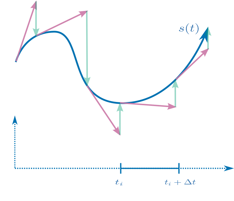
Our task is to numerically continue a known problem/solution pair to a pair for some problem of interest This may be accomplished by introducing a parameter homotopy where is some differentiable function with and The goal is to compute a differentiable path such that and satisfying the implicit equation . Note that the homotopy depends on and that many choices are possible. We mainly consider Linear segment HC: that is, we choose .
In practice, we compute an approximation of the solution curve by numerical predictor/corrector methods, illustrated in Fig. 2(b). In our predictor step, the value for a given is known, and the value for an adaptively-chosen stepsize is approximated using the standard fourth-order Runge-Kutta method. In the corrector step, the value is refined by up to steps of Newton’s method.
For both cases of 5pt and Scranton problems, there are additional polynomial constraints which rule out certain spurious solutions. However, one advantage of our HC method is that, although the vanishing set of the we use is strictly larger than these additional constraints do not need to be explicitly enforced—See SM Section 16
6.1 Efficient HC implementation
Our work builds on the core of an optimized HC solver introduced in TRPLP that was originally developed for the problem of computing the relative pose of three calibrated cameras from corresponding point-line incidences. The optimized solver in that work is globally convergent with probability , but needs about miliseconds to track complex solution paths to solve a single problem instance.
By contrast, our solver for Scranton tracks a single path in under 10 microseconds, a speedup of more than . As noted in Section 1.3, much of this dramatic speedup is because global HC methods must compute all solutions over the complex numbers, whereas our method computes one, allowing now a greater probability of failure for a given data sample. Moreover, the start system in our HC method is tailored to the input by the anchor selection procedure.
There are also significant implementation-specific speedups. For instance, we obtain another speedup by performing all computations in real, instead of complex arithmetic. We also obtain an speedup by optimizing the linear algebra underlying predictor/corrector steps; the Jacobian matrices of our depth-formulated are sparse, leading to inexpensive closed-form solutions.88 8 See SM Sec. 16 for more details.
7 Minimal problem formulation
We now describe the polynomial systems used by our 5pt and 4pt HC solvers. The unknowns in both systems are the normalized depths in each camera, as formulated in previous works zhang2011pose; QuanTM2006. We choose this formulation over others because (i) due to low degree and sparsity, it leads to fast evaluation of straight-line programs and fast execution of linear algebra subroutines used in homotopy tracking and (ii) it works well in tandem with our normalization procedure described in Section 8.
To derive polynomial constraints relating depths and image points, consider two 3D points labeled by that are projected by two calibrated cameras labeled by into image points with the corresponding homogeneouos coordinates given by . We see, Fig. 3, that must hold, where the unknown is the depth of the 3D point in camera . This constraint means that the distance between every two 3D points, when reconstructed in different cameras, must be the same.
7.1 5pt minimal problem
The 5pt problem is parametrized by the projection of 5 3D points into 2 calibrated cameras. There are unknown depths , , , and equations
| (1) |
, . To dehomogenize this system, we set to obtain a system of equations in unknowns. It has solutions for generic parameters . There are two isolated singular solutions , with multiplicity , and isolated nonsingular solutions. Among the nonsingular solutions, there are at most with all depths positive which extend to a rotation with .
For our HC solver, we have to select a square subsystem, i.e., 9 equations for 9 unknowns. For generic parameters, any equation can be dropped to get a square system with solutions, where the two singular solutions have multiplicity and the number of nonsingular solutions rises to . As noted in Section 6, the dropped equation and other polynomial constraints () need not be explicitly enforced by our HC solver.99 9 See SM Sec. 14 for additional details about the problem formulation..
7.2 Scranton relaxation of the 4pt problem
The 4pt problem consists of the projection of 4 points into 3 calibrated cameras. Therefore, it involves unknown depths , , , and equations. However, only 2 equations, from each equations involving the same pair of 3D points, are independent. Hence we get equations
| (2) |
, and, e.g., , . To dehomogenize the system, we set . Unlike for the 5pt problem, here we get an overconstrained system of equations for unknown depths, which has no solution for generic (noisy) parameters . To get a minimal problem, we replace by , where is a new unknown. This relaxation allows us to “adjust” the second coordinate of the first point in the first camera. Notice that by relaxing the first point in the first view, which has , the equations involving that point
for remain quadratic in unknowns Solutions to the minimal problem “Scranton”, Fig. 3, are solutions to this square, inhomogeneous system of polynomials used in our HC solver.1010 10 See SM Sec. 15 for additional details about Scranton..
8 Problem preprocessing
To simplify both the learning the anchor selection strategy and the HC tracking, we considered several schemes for normalizing the input image correspondences, i.e., the parameters of the problems. Our chosen normalization yields single representative for all problems that differ from up to camera re-orientation or permutation of cameras or correspondences. Once the normalized problem is solved, the original problem may be solved by applying a transformation described below.
For the 5pt problem, a problem is given by image coordinates with cameras indexed by and points indexed by . First, we construct unit 3D vectors representing the rays of the image points as . Next, we compute the mean ray for each camera . Then, we find the ray that contains the largest angle with the mean ray of its camera, i.e., . Next, we compute such that and , as well as the corresponding , have the second coordinate equal to , i.e., we put them on the “ axis”. Finally, we swap the cameras to make the camera the first one, project 3D rays back to the image points , and reorder the image correspondences counterclockwise starting with 1111 11 See SM Fig. 8 for an example of image correspondences after the normalization, and SM Sec. 17 for a comparison with other normalizations which delivered worse results in our evaluation..
For the 4pt problem, cameras are ordered according to angles of the first point;
9 Experiments - RANSAC evaluation

To show how our method generalizes to different real scenes and to data contaminated by noise and wrong matches, we evaluate our approach for the 5pt problem on the dataset from the CVPR 2020 RANSAC Tutorial ransac_tutorial consising of 2 validation scenes and 11 test scenes, each comprising 4950 camera pairs. For every camera pair, a set of matched 2D points is known. The points are contaminated with noise and mismatches. We evaluate solvers by plugging them into a RANSAC scheme Raguram-USAC-PAMI-2013 and computing relative poses for camera pairs in each scene. We evaluate the rotation error and translation error separately. Our evaluation metric is the percentage of relative poses whose angular distance from the ground truth is less than . We believe that this metric is justified, because the main purpose of the RANSAC procedure is to separate the correct matches from the mismatches, and a more precise relative pose can be obtained by local optimization on the inliers.
We consider our HC solver with a single anchor, our HC solver with MLP without trash, and our HC solver with MLP and trash. To estimate the success rate of our solver on this data, we compare it with the Nistér 5 point solver Nister-5pt-PAMI-2004. The success rate of the Nistér solver is close to , and its errors are only due to the noise and mismatches in the data. Therefore, if the success rate of a solver on the given data is, e.g., , we expect it to need 4 times the number of samples used for the Nistér solver to get the same results. We have considered RANSAC with and samples. The inlier ratio is px. The relation between the number of samples and the percentage of correctly estimated cameras is shown in Fig. 4. The graph shows that the lower success rate of our method can be compensated by running RANSAC for more samples. Our method with MLP requires about 4 times more samples than the Nistér solver. Therefore, the success rate on the data from ransac_tutorial is around , which is about times lower than the success rate on the testing data from ETH 3D dataset
1212
12
See SM Sec. 18 for the study of our engineering choices..
10 Conclusion
Our approach to solving hard minimal problems for RANSAC framework, which uses efficient homotopy continuation and machine learning to avoid solving for many spurious solutions, is fast and delivers correct results. Supplementary Material (SM) presents more details and experiments. Our code and and data are available at https://github.com/petrhruby97/learning_minimal
Limitations of our approach: First, we sacrifice the high success rate of a complex HC method for a fast, real HC method that fails more frequently. Nevertheless, when combined with trained models, our method succeeds in computing real solutions often enough to be useful in RANSAC. Secondly, our MLP model represents only what it is trained for. Still, we saw that it was able to represent real data distributions while keeping small size and fast evaluation. Fitting to a particular data distribution may also be useful in special situations, e.g., when cameras are mounted on a vehicle, hence having special motions.
References
- (1) Sameer Agarwal, Hon-leung Lee, Bernd Sturmfels, and Rekha R. Thomas. On the existence of epipolar matrices. International Journal of Computer Vision, 121(3):403–415, 2017.
- (2) Chris Aholt and Luke Oeding. The ideal of the trifocal variety. Math. Comput., 83(289):2553–2574, 2014.
- (3) Hatem Said Alismail, Brett Browning, and M Bernardine Dias. Evaluating pose estimation methods for stereo visual odometry on robots. In the 11th International Conference on Intelligent Autonomous Systems (IAS-11), January 2011.
- (4) Daniel Barath. Five-point fundamental matrix estimation for uncalibrated cameras. In 2018 IEEE Conference on Computer Vision and Pattern Recognition, CVPR 2018, Salt Lake City, UT, USA, June 18-22, 2018, pages 235–243, 2018.
- (5) Daniel Barath and Levente Hajder. Efficient recovery of essential matrix from two affine correspondences. IEEE Trans. Image Processing, 27(11):5328–5337, 2018.
- (6) Daniel Barath, Tekla Toth, and Levente Hajder. A minimal solution for two-view focal-length estimation using two affine correspondences. In 2017 IEEE Conference on Computer Vision and Pattern Recognition, CVPR 2017, Honolulu, HI, USA, July 21-26, 2017, pages 2557–2565, 2017.
- (7) Daniel J. Bates, Andrew J. Sommese, Jonathan D. Hauenstein, and Charles W. Wampler. Numerically Solving Polynomial Systems with Bertini, volume 25 of Software, environments, tools. SIAM, 2013.
- (8) Snehal Bhayani, Zuzana Kukelova, and Janne Heikkilä. A sparse resultant based method for efficient minimal solvers. In 2020 IEEE/CVF Conference on Computer Vision and Pattern Recognition, CVPR 2020, Seattle, WA, USA, June 13-19, 2020, pages 1767–1776. IEEE, 2020.
- (9) G. Bradski. The OpenCV Library. Dr. Dobb’s Journal of Software Tools, 2000.
- (10) Paul Breiding and Sascha Timme. Homotopycontinuation.jl: A package for homotopy continuation in julia. In James H. Davenport, Manuel Kauers, George Labahn, and Josef Urban, editors, Mathematical Software - ICMS 2018 - 6th International Conference, South Bend, IN, USA, July 24-27, 2018, Proceedings, volume 10931 of Lecture Notes in Computer Science, pages 458–465. Springer, 2018.
- (11) Martin Byröd, Klas Josephson, and Kalle Åström. A column-pivoting based strategy for monomial ordering in numerical Gröbner basis calculations. In European Conference on Computer Vision (ECCV), volume 5305, pages 130–143. Springer, 2008.
- (12) F. Camposeco, T. Sattler, and M. Pollefeys. Minimal solvers for generalized pose and scale estimation from two rays and one point. In ECCV – European Conference on Computer Vision, pages 202–218, 2016.
- (13) David Cox, John Little, and Donald O’Shea. Using Algebraic Geometry. Springer, 1998.
- (14) Timothy Duff, Cvetelina Hill, Anders Jensen, Kisun Lee, Anton Leykin, and Jeff Sommars. Solving polynomial systems via homotopy continuation and monodromy. IMA Journal of Numerical Analysis, 2018.
- (15) T. Duff, K. Kohn, A. Leykin, and T. Pajdla. PLMP - point-line minimal problems in complete multi-view visibility. In 2019 IEEE/CVF International Conference on Computer Vision (ICCV), pages 1675–1684, 2019.
- (16) Timothy Duff, Kathlén Kohn, Anton Leykin, and Tomás Pajdla. PLP - point-line minimal problems under partial visibility in three views. In Andrea Vedaldi, Horst Bischof, Thomas Brox, and Jan-Michael Frahm, editors, Computer Vision - ECCV 2020 - 16th European Conference, Glasgow, UK, August 23-28, 2020, Proceedings, Part XXVI, volume 12371 of Lecture Notes in Computer Science, pages 175–192. Springer, 2020.
- (17) Timothy Duff, Viktor Korotynskiy, Tomas Pajdla, and Margaret H Regan. Galois/monodromy groups for decomposing minimal problems in 3d reconstruction. arXiv preprint arXiv:2105.04460, 2021.
- (18) Ali Elqursh and Ahmed M. Elgammal. Line-based relative pose estimation. In The 24th IEEE Conference on Computer Vision and Pattern Recognition, CVPR 2011, Colorado Springs, CO, USA, 20-25 June 2011, pages 3049–3056. IEEE Computer Society, 2011.
- (19) Ioannis Z. Emiris. A general solver based on sparse resultants. CoRR, abs/1201.5810, 2012.
- (20) Ricardo Fabbri, Timothy Duff, Hongyi Fan, Margaret H. Regan, David da Costa de Pinho, Elias P. Tsigaridas, Charles W. Wampler, Jonathan D. Hauenstein, Peter J. Giblin, Benjamin B. Kimia, Anton Leykin, and Tomás Pajdla. TRPLP - Trifocal relative pose from lines at points. In 2020 IEEE/CVF Conference on Computer Vision and Pattern Recognition, CVPR 2020, Seattle, WA, USA, June 13-19, 2020, pages 12070–12080. IEEE, 2020.
- (21) R. Fabbri, P. Giblin, and B. Kimia. Camera pose estimation using first-order curve differential geometry. IEEE Transactions on Pattern Analysis and Machine Intelligence, 2020.
- (22) Jean-Charles Faugère, Guillaume Moroz, Fabrice Rouillier, and Mohab Safey El Din. Classification of the perspective-three-point problem, discriminant variety and real solving polynomial systems of inequalities. In J. Rafael Sendra and Laureano González-Vega, editors, Symbolic and Algebraic Computation, International Symposium, ISSAC 2008, Linz/Hagenberg, Austria, July 20-23, 2008, Proceedings, pages 79–86. ACM, 2008.
- (23) M. A. Fischler and R. C. Bolles. Random sample consensus: a paradigm for model fitting with applications to image analysis and automated cartography. Commun. ACM, 24(6):381–395, 1981.
- (24) Phillip Griffiths and Joseph Harris. Principles of algebraic geometry. Wiley Classics Library. John Wiley & Sons, Inc., New York, 1994. Reprint of the 1978 original.
- (25) J. A. Grunert. Das pothenotische Problem in erweiterter Gestalt nebst über seine Anwendungen in Geodäsie. In Grunerts Archiv für Mathematik und Physik, 1841.
- (26) Robert M. Haralick, Chung-Nan Lee, Karsten Ottenberg, and Michael Nölle. Review and analysis of solutions of the three point perspective pose estimation problem. Int. J. Comput. Vis., 13(3):331–356, 1994.
- (27) R. Hartley and Hongdong Li. An efficient hidden variable approach to minimal-case camera motion estimation. IEEE PAMI, 34(12):2303–2314, 2012.
- (28) Richard Hartley and Andrew Zisserman. Multiple View Geometry in Computer Vision. Cambridge, 2nd edition, 2003.
- (29) Janne Heikkilä. Using sparse elimination for solving minimal problems in computer vision. In IEEE International Conference on Computer Vision, ICCV 2017, Venice, Italy, October 22-29, 2017, pages 76–84. IEEE Computer Society, 2017.
- (30) Robert J. Holt and Arun N. Netravali. Uniqueness of solutions to three perspective views of four points. IEEE Trans. Pattern Anal. Mach. Intell., 17(3):303–307, 1995.
- (31) Joe Kileel. Minimal problems for the calibrated trifocal variety. SIAM Journal on Applied Algebra and Geometry, 1(1):575–598, 2017.
- (32) L. Kneip, D. Scaramuzza, and R. Siegwart. A novel parametrization of the perspective-three-point problem for a direct computation of absolute camera position and orientation. In CVPR – IEEE Conference on Computer Vision and Pattern Recognition, pages 2969–2976, 2011.
- (33) L. Kneip, R. Siegwart, and M. Pollefeys. Finding the exact rotation between two images independently of the translation. In ECCV – European Conference on Computer Vision, pages 696–709, 2012.
- (34) Yubin Kuang and Kalle Åström. Pose estimation with unknown focal length using points, directions and lines. In IEEE International Conference on Computer Vision, ICCV 2013, Sydney, Australia, December 1-8, 2013, pages 529–536, 2013.
- (35) Yubin Kuang and Kalle Åström. Stratified sensor network self-calibration from TDOA measurements. In 21st European Signal Processing Conference, 2013.
- (36) Zuzana Kukelova, Martin Bujnak, and Tomas Pajdla. Automatic generator of minimal problem solvers. In European Conference on Computer Vision (ECCV), 2008.
- (37) Zuzana Kukelova, Martin Bujnak, and Tomas Pajdla. Polynomial eigenvalue solutions to minimal problems in computer vision. IEEE Transactions on Pattern Analysis and Machine Intelligence, 2012.
- (38) Viktor Larsson. PoseLib - Minimal Solvers for Camera Pose Estimation, 2020.
- (39) Viktor Larsson, Kalle Åström, and Magnus Oskarsson. Efficient solvers for minimal problems by syzygy-based reduction. In Computer Vision and Pattern Recognition (CVPR), 2017.
- (40) Viktor Larsson, Kalle Åström, and Magnus Oskarsson. Polynomial solvers for saturated ideals. In IEEE International Conference on Computer Vision, ICCV 2017, Venice, Italy, October 22-29, 2017, pages 2307–2316, 2017.
- (41) Viktor Larsson, Zuzana Kukelova, and Yinqiang Zheng. Making minimal solvers for absolute pose estimation compact and robust. In International Conference on Computer Vision (ICCV), 2017.
- (42) Viktor Larsson, Magnus Oskarsson, Kalle Åström, Alge Wallis, Zuzana Kukelova, and Tomás Pajdla. Beyond grobner bases: Basis selection for minimal solvers. In 2018 IEEE Conference on Computer Vision and Pattern Recognition, CVPR 2018, Salt Lake City, UT, USA, June 18-22, 2018, pages 3945–3954, 2018.
- (43) Anton Leykin. Numerical algebraic geometry. Journal of Software for Algebra and Geometry, 3(1):5–10, 2011.
- (44) Pedro Miraldo, Tiago Dias, and Srikumar Ramalingam. A minimal closed-form solution for multi-perspective pose estimation using points and lines. In Computer Vision - ECCV 2018 - 15th European Conference, Munich, Germany, September 8-14, 2018, Proceedings, Part XVI, pages 490–507, 2018.
- (45) Faraz M Mirzaei and Stergios I Roumeliotis. Optimal estimation of vanishing points in a manhattan world. In International Conference on Computer Vision (ICCV), 2011.
- (46) A. Morgan. Solving Polynomial Systems Using Continuation for Engineering and Scientific Problems. Classics in Applied Mathematics. Society for Industrial and Applied Mathematics (SIAM, 3600 Market Street, Floor 6, Philadelphia, PA 19104), 2009.
- (47) Dmytro Myshkin. Benchmarking robust estimation methods. Tutorial “RANSAC in 2020”, CVPR, 2020.
- (48) D. Nistér. An efficient solution to the five-point relative pose problem. IEEE Transactions on Pattern Analysis and Machine Intelligence, 26(6):756–770, June 2004.
- (49) David Nistér, Oleg Naroditsky, and James Bergen. Visual odometry. In Computer Vision and Pattern Recognition (CVPR), pages 652–659, 2004.
- (50) David Nistér and Frederik Schaffalitzky. Four points in two or three calibrated views: Theory and practice. International Journal of Computer Vision, 67(2):211–231, 2006.
- (51) Mikael Persson and Klas Nordberg. Lambda twist: An accurate fast robust perspective three point (P3P) solver. In Vittorio Ferrari, Martial Hebert, Cristian Sminchisescu, and Yair Weiss, editors, Computer Vision - ECCV 2018 - 15th European Conference, Munich, Germany, September 8-14, 2018, Proceedings, Part IV, volume 11208 of Lecture Notes in Computer Science, pages 334–349. Springer, 2018.
- (52) Long Quan, Bill Triggs, and Bernard Mourrain. Some results on minimal euclidean reconstruction from four points. Journal of Mathematical Imaging and Vision, 24(3):341–348, 2006.
- (53) R. Raguram, O. Chum, M. Pollefeys, J. Matas, and J.-M. Frahm. USAC: A universal framework for random sample consensus. IEEE Transactions on Pattern Analysis Machine Intelligence, 35(8):2022–2038, 2013.
- (54) S. Ramalingam and P. F. Sturm. Minimal solutions for generic imaging models. In CVPR – IEEE Conference on Computer Vision and Pattern Recognition, 2008.
- (55) Ignacio Rocco, Mircea Cimpoi, Relja Arandjelović, Akihiko Torii, Tomas Pajdla, and Josef Sivic. Neighbourhood consensus networks, 2018.
- (56) Yohann Salaün, Renaud Marlet, and Pascal Monasse. Robust and accurate line- and/or point-based pose estimation without manhattan assumptions. In European Conference on Computer Vision (ECCV), 2016.
- (57) Torsten Sattler, Bastian Leibe, and Leif Kobbelt. Efficient & effective prioritized matching for large-scale image-based localization. IEEE Trans. Pattern Anal. Mach. Intell., 39(9):1744–1756, 2017.
- (58) Olivier Saurer, Marc Pollefeys, and Gim Hee Lee. A minimal solution to the rolling shutter pose estimation problem. In Intelligent Robots and Systems (IROS), 2015 IEEE/RSJ International Conference on, pages 1328–1334. IEEE, 2015.
- (59) Johannes Lutz Schönberger and Jan-Michael Frahm. Structure-from-motion revisited. In Conference on Computer Vision and Pattern Recognition (CVPR), 2016.
- (60) Thomas Schöps, Johannes L. Schönberger, Silvano Galliani, Torsten Sattler, Konrad Schindler, Marc Pollefeys, and Andreas Geiger. A multi-view stereo benchmark with high-resolution images and multi-camera videos. In Conference on Computer Vision and Pattern Recognition (CVPR), 2017.
- (61) N. Snavely, S. M. Seitz, and R. Szeliski. Photo tourism: exploring photo collections in 3D. In ACM SIGGRAPH, 2006.
- (62) Noah Snavely, Steven M Seitz, and Richard Szeliski. Modeling the world from internet photo collections. International Journal of Computer Vision (IJCV), 80(2):189–210, 2008.
- (63) Andrew J. Sommese and Charles W. Wampler II. The numerical solution of systems of polynomials - arising in engineering and science. World Scientific, 2005.
- (64) H. Stewenius, C. Engels, and D. Nistér. Recent developments on direct relative orientation. ISPRS J. of Photogrammetry and Remote Sensing, 60:284–294, 2006.
- (65) Bernd Sturmfels. Solving Systems of Polynomial Equations, volume 97 of CBMS Regional Conferences Series. Amer.Math.Soc., Providence, Rhode Island, 2002.
- (66) Hajime Taira, Masatoshi Okutomi, Torsten Sattler, Mircea Cimpoi, Marc Pollefeys, Josef Sivic, Tomas Pajdla, and Akihiko Torii. InLoc: Indoor visual localization with dense matching and view synthesis. In CVPR, 2018.
- (67) Jonathan Ventura, Clemens Arth, and Vincent Lepetit. An efficient minimal solution for multi-camera motion. In International Conference on Computer Vision (ICCV), pages 747–755, 2015.
- (68) Jan Verschelde. Polynomial homotopy continuation with phcpack. ACM Commun. Comput. Algebra, 44(3/4):217–220, 2010.
- (69) Ji Zhang, Mireille Boutin, and Daniel G Aliaga. Pose-free structure from motion using depth from motion constraints. IEEE transactions on image processing, 20(10):2937–2953, 2011.
Supplementary Material
Here we give additional details, including an analysis of the 5pt and Scranton minimal problem solutions, details of our efficient homotopy continuation implementation, and experiments justifying our engineering choices. Our code is available at https://github.com/petrhruby97/learning_minimal
11 A classical example of a minimal problem
A classical, easy, but still essential, minimal problem in computer vision is computing the pose of a calibrated perspective camera HZ-2003 from three points in space and their image projections Grunert-1841; DBLP:journals/ijcv/HaralickLON94; DBLP:conf/cvpr/KneipSS11; larsson2017making; DBLP:conf/eccv/PerssonN18. In one of its classical formulations Grunert-1841, it leads to a polynomial system of three equations
of degree two in three unknown depths . Parameters of the problem are three 3D points and homogeneous coordinates of three image projections, altogether on parameters. For generic data, the system has eight complex solutions for ’s with up to eight real solutions DBLP:conf/issac/FaugereMRD08. However, often, there are only zero, two, or four real solutions with positive ’s.
This example illustrates a typical situation occurring in minimal problem solving. The minimal problem obtained by relaxing a geometrical optimization problem, which has one optimal solution, brings in seven additional (spurious) solutions. In this case, there are always at least two real solutions corresponding to seeing the three points from the opposite sides of the plain they span.
12 Interesting hard minimal problems
Recent results PLMP; PL1P suggest that solving minimal problems with many complex solutions is interesting. A complete classification of minimal problems for points, lines, and their incidences in the calibrated multi-view geometry appeared for the case of complete multi-view visibility PLMP. It has been found that there are only 30 minimal problems in that setting, but it also became clear that problems involving more than two cameras are hard for the current symbolic-numeric and homotopy continuation solvers. The number of solutions for three views starts with 64, interesting cases have 200+ solutions, and 5-view cases have 10000+ solutions. Allowing for occlusion or missed detection in images leads to even harder problems. The follow-up work PL1P developed a complete classification of minimal problems for generic arrangements of points and lines in space, observed partially by three calibrated perspective cameras when each line is incident to at most one point. It has been found that there is an infinite number of such minimal problems arranged into 74575 equivalence classes when caring only about camera configurations. Interestingly, this classification involves all calibrated trifocal geometry of computer vision for nonincident points and lines in space. Out of 74575 classes, only 759 classes have less than 300 solutions. The rest have (many) more solutions. Thus, for many interesting and potentially practical problems, computing all solutions in a reasonable time is a task beyond the reach of current symbolic-numeric and homotopy continuation solving methods.

13 Examples of problem-solution manifolds worked out in detail
Let us now provide a detailed explanation of the problem-solution manifold concept introduced in Sec. 2.1 for the 5pt and 4pt problems solved in this work.
Example 3.
Consider the 5pt problem of computing the relative pose of two calibrated cameras from 5 correspondences in two images,i.e., two matrices in the special Euclidean group , which view five world points where is normalized to lie in the first image plane: The points are in front of both cameras iff their depths
are all positive ( is the third row of and the third entry of .) Consider
where
| (3) |
Here the problem space is the solution space is , , and our problem-solution manifold is the set of smooth points in the semialgebraic set
Remark 1.
For a generic problem the fiber consists of at most solutions , and every such can be extended uniquely to a pair
Remark 2.
Our assumptions in Example 3 imply that In subsequent sections, we treat the five-point problem as a system of equations in the nine remaining unknown depths. More generally, we could dehomogenize our system by setting any linear form in ’s equal to
Example 4.
Consider the Scranton relaxation of the 4pt problem computing the relative pose of three calibrated cameras from 4 correspondences in 3 images. We have 4 world points with and three cameras such that cameras view cameras view and camera views the line in the direction that passes through parametrized as Now, we have a map
where are as in Eq. 3 except that
Here the problem space is the solution space is , , and our problem-solution manifold is the set of smooth points in the semialgebraic set
14 Additional details for 5pt formulation
Here we provide additional details concerning the solutions of the depth-formulated 5pt problem developed in Section 7.1. Given we first note that a valid rotation matrix may be estimated by computing certain auxiliary quantites: for and we define and, for distinct
Thus, gives the oriented volume of a tetrahedron whose vertices are To estimate the rotation from a geometrically meaningful solution, one may compute either
| (4) |
or
| (5) |

The solutions to Equation 1 need not satisfy the additional constraint , since there is a sign-symmetry which changes the sign of but leaves Equation 1 invariant. Moreover, there are nonsingular, spurious solutions to the square subsystem obtained by dropping one equation, plus an additional of higher multiplicity. For these spurious solutions, either of the matrices in Eq. 4 or Eq. 5 may have determinant These spurious solutions may be ruled out by enforcing for either both of these matrices, or for one of these matrices in addition to all original depth constraints. With these constraints enforced, the generic number of solutions drops to Moreover, there is an additional symmetry given by the “twisted pair” HZ-2003: letting
we define coordinate-wise fixing and
The map on p-s pairs reverses the signs of depths in the second view. This justifies our claim that there are at most geometrically meaningful solutions to Eq. 1. We remark that the partition of solutions into twisted pairs is preserved along non-singular solution curves computed by our HC method.
15 Additional details for Scranton formulation
Unlike the system used for the 5pt problem, the square system for Scranton has infinitely many solutions. Recall that this system is given by the relaxed depth constraint
and Eq. 2 for remaining points and cameras. A one-dimensional family of solutions may be obtained by setting all depths except to resulting in nontrivial equations in the remaining unknowns: namely,
The square system for Scranton also has several families of isolated singular solutions where certain depths equal However, for generic data, the number of nonsingular solutions equals the number of solutions with nonzero depths, which is Among these, there is a four-fold sign symmetry where and cannot be lifted to a valid pair of rotations
Taking these facts into account, there are at most geometrically relevant solutions on the problem-solution manifold. This agrees with the number of solutions reported in both Kileel-MPCTV-2016 and PL1P, where formulations in terms of trifocal tensors and camera matrices, respectively, were employed. We note that, unlike the five-point problem, there is no further reduction in the number of solutions implied by a symmetry such as the twisted pair; this follows by numerically computing the Galois group associated to Scranton, using techniques described in duff2021galois, which turns out to be the symmetric group on letters.

16 Additional details on HC methods
As noted in Section 6, our homotopy depends on the choice of a path connecting to where is a known p-s pair and is the problem to be solved. In all of our experiments, we consider one of two choices. Mostly, we use 1) Linear segment HC: that is, we choose . This linear segment homotopy has several advantages; among them, the straight-line programs needed to evaluate and its derivatives are much simpler than for other paths, and the fact that is real-valued for all However, under Linear segment HC, a differentiable solution curve satisfying need not exist for all . For instance, a problem with singular solutions may exist somewhere along the segment connected in connecting and However, the solution curve will exist for all if and are “close enough”—more precisely, if avoids the lower-dimensional set of critical values of in for all
Alternatively, one may consider 2) Circular arc HC: here, we reparametrize the segment via a circular arc obtained by fixing a random (typically of modulus ) and . This is the -trick of (DBLP:books/daglib/0014410, Lemma 7.1.3 ). Numerical continuation with the resulting homotopy is globally convergent with probability one: for almost all choices of the solution curves are defined for all and any isolated target solution is the endpoint of some solution curve. However, this necessitates computing many spurious solutions. An experimental comparison of Linear segment and Circular arc HC may be found in Table 7.
We now explain why the square systems used in our homotopies are sufficient when starting from a p-s pair on the problem-solution manifold. Consider a path where and such that that the Jacobian matrix has rank for all Thus, the path is contained in a single connected component of the set of nonsingular points in the complex vanishing set Among these connected components is the set of smooth points in the Zariski closure of . Indeed, the complex Zariski closure of has a rational parametrization (given by one of the maps defined in Section 13), so it is irreducible, and the connectedness of its smooth points follows by (GriffHarr, pp. 21–22). Since the point is contained in this connected component, so also must for all Thus, any polynomial vanishing on satisfies for all This means that, if HC tracking from succeeds using our square system of constraints, then all additional constraints which are polynomial equalities are automatically satisfied. This justifies the fact that we do not explicitly enforce constraints like , since it is enough to enforce them for the initial p-s pair.
16.1 Efficient evaluation of predictor/corrector
The Runge-Kutta method used for the predictor step and Newton’s method used for the corrector step in our HC implementation both require solving systems of linear equations. In either step, the coefficient matrix is given by the Jacobian (Sec. 6). In the case of the depth formulation of the Five-Point problem (1) and the Four-Point problem (2), the associated Jacobian matrix is sparse. The sparsity pattern of the Jacobian matrix is shown in (6) for the Five-Point problem, and in (7) for the Four-Point problem.
| (6) |
| (7) |
Using generic methods such as LU decomposition, as in previous work Fabbri-PAMI-2020, numerical linear algebra becomes a significant bottleneck in both the predictor and corrector stages. To overcome this bottleneck, we replace the generic numerical linear algebra with closed-form solutions to the systems of linear equations with coefficient matrices (6) and (7). This replacement results in about 5x speedup for both problems.
17 Variations of the normalization
Let us provide additional details about our normalization of problems to simplify their variability and thus to make learning of the picking function easier.
Fig. 8 shows an example of the normalized 5pt problem. The mean direction vectors in both images are at . The first correspondence, is on the axis. The first image is chosen such that it contains the larger angle with its corresponding . This also means that the first correspondence point has a larger image coordinate: . To make the normalized problems independent on the ordering of the correspondences, we sort them by their polar angles in the coordinate system in the the first image. Notice that their order may be swapped in the second image, e.g., as for , . Such a swap is mainly due to a large change of the order of depth of the corresponding points in the scene, as seen from different view points, which is in practice much less frequent than keeping the order [70].
Our normalization is chosen as the best one among several meaningful alternatives. The evaluation of the alternative normalization methods is shown in Tab. 5 for the 5pt problem and in Tab. 6 for the Scranton problem. The tables show that our strategy, labeled by A, which rotates the center of mass to zero and the farthest point on the -axis, has the best success rate for both problems. Note that every normalization strategy performs better than when tracking without normalization.
The normalization strategies are as follows:
- 1.
Rotate the center of mass to zero, rotate the point farthest from zero to -axis.
- 2.
Rotate the center of mass to zero with an iterative procedure, rotate the point farthest from zero to -axis.
- 3.
Rotate the closest point to center of mass to zero and the point farthest from zero to -axis.
- 4.
Rotate the center of mass to zero and the maximal variance to -axis.
- 5.
Rotate the closest point to center of mass to zero and the maximal variance to -axis.
In the case of the Scranton problem, we also have to decide which point in which view to relax on the line. Here, we consider:
- 1.
The farthest point and view.
- 2.
The point rotated to zero (if possible).
Our normalization induces three linear constraints for every view. The instance of the 5pt problem consists of 2D projections of 5 points into two views, therefore . The normalized instances live in a dimensional subspace of . The instance of the 4pt problem consists of 2D projections of 4 points into 3 views, . The normalized instances live in a dimensional subspace of .
The values of the success rate in this experiment are low because we use randomly sampled data and track from every p-s pair to every other p-s pair. Tab. 9 shows that the success rate significantly increases if we track from preselected anchors which are chosen to perform well and we select the best starting anchor with a trained classifier.
| Strategy | Succ. rate | Time inv. | Time HC |
|---|---|---|---|
| No inv. | 0.53% | 0 | 14.25 |
| A. | 3.73% | 0.43 | 11.80 |
| B. | 3.70% | 0.77 | 11.88 |
| C. | 2.29% | 0.36 | 11.19 |
| D. | 1.56% | 1.03 | 12.18 |
| E. | 0.71% | 0.68 | 10.44 |
| Strategy | Line strategy | Succ. rate | Time inv. | Time HC |
|---|---|---|---|---|
| No inv. | - | 0.21% | 0 | 22.11 |
| A. | a) | 1.44% | 0.50 | 17.82 |
| B. | a) | 1.44% | 1.16 | 17.40 |
| C. | a) | 0.80% | 0.82 | 19.57 |
| C. | b) | 0.32% | 0.78 | 17.37 |
| D. | a) | 0.61% | 1.39 | 20.13 |
| E. | a) | 0.37% | 1.01 | 20.43 |
| E. | b) | 0.27% | 0.93 | 18.46 |
18 Study to justify engineering choices
Let us describe the data sets we use to study our engineering choices.
Training data set consists of 40000 p-s pairs. We randomly sample pairs of cameras and 5-tuples of 3D points from the ETH 3D dataset schoeps2017cvpr “Office” and “Terrains”. Problem parameters are 10D vectors of 2D image coordinates obtained by projecting the sampled 5-tuples of 3D points by the camera pairs. The corresponding solutions are 10D vectors of the depths of the 3D points in the two cameras normalized to have the first depth equal to 1. Data set , consisting of 40000 p-s pairs, is constructed analagously by sampling 4-tuples of 3D points and triplets of cameras. Data sets are used to select anchor sets and to train our model for selecting the starting problem-solution pair.
Anchor sets are selected by the procedure described in Sec. 4 such that where of anchors covers 50% of problems in , of 26 anchors covers 75% of problems in , of 70 anchors covers 90% of problems in and of 465 anchors covers 100% of problems in . Data sets, , of 16 anchors, , of 50 anchors, , of anchors and , of 1205 anchors, are constructed analagously from .
Test data set consists of 60000 p-s pairs constructed as above from the ETH 3D dataset “Delivery area” and “Facade”. Data set , consisting of 60000 p-s pairs, is constructed analagously. We use and in the experiments studying anchor set selection methods reported in Tab. 4.
| Succ. rate [%] / Time [] | |||
|---|---|---|---|
| 5pt problem | |||
| Solving technique | M2 leykin2011numerical | MINUS TRPLP | OUR |
| -HC, All Sols | 98.9 0.2/ | 97.7 0.2 / 15197.1 | 97.7 0.1 / 5133.7 |
| -HC, Sols | 56.1 3.3 / | 55.3 2.6 / 5704.7 | 54.7 3.2 / 1895.1 |
| -HC, Fab Sol | / | 12.0 1.5 / 638.0 | 13.1 1.4 / 165.8 |
| -HC, Sols | 9.9 1.7 / | 9.7 1.5 / 647.9 | 9.7 1.5 / 106.8 |
| -HC, Fab Sol | 3.4 1.3 / | 2.7 0.8 / 67.6 | 2.7 0.8 / 11.1 |
| Newton, Fab Sol | 4.0 0.6 / | 4.0 0.7 / 8.5 | 4.0 0.7 / 1.3 |
| Succ. rate [%] / Time [] | ||
|---|---|---|
| Scranton | ||
| Solving technique | MINUS TRPLP | OUR |
| -HC, All Sols | 95.5 2.6 / 608332.0 | 95.7 2.6 / 187364.5 |
| -HC, Sols | 22.7 1.6 / 47961.4 | 22.5 1.7 / 14905.1 |
| -HC, Fab Sol | 3.5 0.7 / 1280.7 | 3.3 0.9 / 405.7 |
| -HC, Sols | 7.5 1.2 / 2548.4 | 7.6 1.2 / 484.4 |
| -HC, Fab Sol | 1.2 0.3 / 70.2 | 1.2 0.3 / 14.1 |
| Newton, Fab Sol | 1.9 0.6 / 8.6 | 2.0 0.4 / 1.4 |
18.1 Comparison of different tracking approaches
Data set consists of of 3751 p-s pairs sampled from the ETH 3D dataset “Courtyard”. and are disjoint. All problems in are checked to be generic and can be used as good starting problem-solution pairs. We select 20 random pairwise disjoint consisting of problem-solution pairs. Data sets , consisting of 5727 problem-solutions pairs, and , consisting of 50 p-s pairs, are constructed analagously. We use ’s and in the experiments studying variations of the homotopy continuation methods reported in Tab. 7. In this table, we measure the success rate for a given subset as a percentage of different pairs for which the fabricated solution to the target problem can be recovered when tracking from to . Then, we find the mean success rate , and the standard deviation over all subsets .
Tab. 7 shows that for every setting, our evaluation (Sec. 16.1) brings about 5x speedup over the previous work TRPLP without any impact on the success rate.
The table also shows that Homotopy Continuation in the complex domain tracked from every solution has almost success rate, but the running time of the solver is prohibitively slow to be used in the RANSAC scheme. We can see that reducing the number of tracks, as well as tracking in instead of can significantly reduce the running time (about 10000x for the Scranton problem) at the cost of a lower success rate. Note (Tab. 9), that the issue with the low success rate may be remedied by selecting an appropriate starting problem-solution pair for every target problem .
Tab. 7 also shows that using the Newton method may be a promising approach for solving the minimal problems, as it has a higher success rate and lower running time than Homotopy Continuation with the same setting. Therefore, we have found starting p-s pairs (Sec. 4) and trained the MLP for the Newton method. The comparison of the solvers using the Homotopy Continuation and the Newton method is shown in Tab. 8. We can see that the effective time (the average time needed to obtain one correct solution in the RANSAC scheme) of the solver using Homotopy Continuation is about 2x lower than the effective time of the solver using Newton method. While the solvers using Newton method are faster, the success rate of the solver, which combines Homotopy Continuation and MLP classifier has a higher success rate. The possible explanation for this is that the Newton method behaves “more randomly” than the Homotopy Continuation, and therefore, it is more difficult to train.
| Method | [%] | [] | [] |
|---|---|---|---|
| N3 + B1 | 0.01 | 1.73 | 15159.7 |
| N3 + MLP | 0.12 | 8.2 | 6811.2 |
| N15 + B1 | 2.1 | 2.6 | 119.7 |
| N15 + MLP | 10.6 | 10.6 | 100.0 |
| HC + B1 | 4.2 | 18.7 | 442.1 |
| HC + MLP | 26.3 | 16.2 | 61.6 |
Tab. 9 provides a more detailed analysis of the frequency of different results of real Homotopy Continuation tracked from the fabricated solution. We consider two different settings. In the “All pairs” setting, we track from each to each other . Then, in the MLP setting, we select a starting p-s pair from , and track from to . We measure how often we reach the fabricated solution, non-fabricated meaningful solution, a non-valid solution, and how often HC fails and does not deliver any solution. The table shows that the MLP increases the probability of reaching the fabricated solution about 10x for 5pt and 20x for Scranton. The probability of reaching another meaningful solution increases about 3x for both problems, while the probability of reaching a non-valid solution and the probability of failing decreases.
| All pairs | MLP | |||
|---|---|---|---|---|
| Result [%] | 5 pt | 4 pt | 5pt | 4pt |
| Fabricated sol. | 3.64 | 1.49 | 38.8 | 29.2 |
| 1 rel. pose correct | - | 0.74 | - | 4.53 |
| Other meaningful | 9.50 | 13.43 | 31.6 | 34.2 |
| Sol. with det -1 | 0.00 | 0.00 | 0.00 | 0.00 |
| Sol. with zeros | 0.03 | 1.53 | 0.01 | 0.52 |
| Negative sol. | 0.52 | 10.86 | 0.83 | 8.54 |
| Failed track | 86.31 | 71.94 | 28.8 | 23.0 |
18.2 Comparison of different settings our solver
Here, we show how different settings of the solver influence the resulting success rate , mean running time , and efficient time . We perform this study on our solver for the Scranton problem. For every experiment, we use the settings from the main paper, except that one parameter is varied. The solver uses anchors and it is evaluated on data . Our goal is to show that we have selected the optimal settings for our solver.
We compare different methods of dehomogenizing Scranton problem in Tab. 10. This justifies our choice of fixing the first depth , which gives a superior success rate compared to “symmetric” and “asymmetric” dehomogenization proposed in QuanTM2006.
See Fig. 9 for a code snippet showing the structure of our MLP model. In Tab. 11, we show how the success rate and running time depends on the size of the MLP that is used for the classification of the anchors. Larger networks have a higher success rate. However, the efficient time of the solver with the smaller MLP is better because the time needed for the evaluation of the MLP grows faster than the success rate.
Finally, in Tab. 12, we show how the number of HC tracks per problem influences the success rate , running time , and efficient time . In this experiment, we use the MLP trained in 5, and we perform tracks from anchors with the highest score. We consider the solution successful if at least one track reaches the fabricated solution of the target problem. Much like using larger MLP as Tab. 11, such a strategy involving multiple anchors suggests a future approach to improving our solvers’ success rates. However, we note that the efficient time in Table 12 grows with the number of tracks, since the evaluation time grows faster than the success rate.
| Formulation | Succ. rate |
|---|---|
| First depth fixed | 2.30 % |
| Quan symmetrical QuanTM2006 | 1.47 % |
| Quan asymmetrical QuanTM2006 | 1.13 % |
| Layer size | [%] | [] | [] |
|---|---|---|---|
| 100 | 27.8 | 20.3 | 73.1 |
| 200 | 31.3 | 30.8 | 98.3 |
| 500 | 34.7 | 79.0 | 227.6 |
| # Tracks | [%] | [] | [] |
|---|---|---|---|
| 1 | 29.2 | 19.6 | 67.0 |
| 2 | 37.2 | 33.3 | 89.6 |
| 3 | 42.2 | 45.0 | 106.8 |
| 4 | 45.9 | 60.8 | 132.6 |
| 8 | 56.4 | 118.1 | 209.5 |
| 16 | 67.9 | 245.3 | 361.5 |
References
[70] A.L. Yuille and T. Poggio. A generalized ordering constraint for stereo correspondence. A.I. Memo 777, AI Lab, MIT, 1994.