Quantum advantage in biometric authentication with single photonsPreprint: AIP/123-QED
Abstract
It was recently proposed to use the human visual system’s ability to perform efficient photon counting in order to devise a new biometric methodology. The relevant biometric "fingerprint" is represented by the optical losses light suffers along several different paths from the cornea to the retina. The "fingerprint" is accessed by interrogating a subject on perceiving or not weak light flashes, containing few tens of photons, so that the subject’s visual system works at the threshold of perception, at which regime optical losses play a significant role. Here we show that if instead of weak laser light pulses we use quantum light sources, in particular single-photon sources, we obtain a quantum advantage, which translates into a reduction of the interrogation time required to achieve a desired performance. Besides the particular application on biometrics, our work further demonstrates that quantum light sources can provide deeper insights when studying human vision.
I Introduction
Secure biometric identification Unar; Yang has some analogies to secure transmission of information: in both cases the potential for some impostor to maliciously intervene in the respective process must be avoided. Quantum cryptography Gisin; Pirandola has served as a paradigm of the so-called "quantum advantage", i.e. the security cryptographic key transmission is guaranteed by the laws of quantum physics. In contrast, classical means of information transmission are vulnerable to e.g. eavesdropping.
In a similar fashion, we recently proposed Loulakis a biometric authentication scheme which takes advantage of the human visual system’s ability to perform photon counting. There, the laws of photon statistics and photodetection at the quantum level of a small number of photons are central for the workings of the scheme, providing for an uncompromising security against an impersonator. The relevant "fingerprint" is a physical property of the visual system, including the eyeball, retina and brain. In other words, the biometric authentication process rests on the conscious perception of weak-intensity light, working at the very threshold of visual perception of a specially designed light stimulus. In particular, the "fingerprint" in this method is the optical loss suffered by light along its propagation from the cornea to the retina.
In our previous work Loulakis the visual stimulus was supposed to originate from laser light. However, the number of photons in a pulse of laser light is known to fluctuate from pulse to pulse around a mean value, and these Poissonian fluctuations limit the performance of the authentication process as will be outlined later. Interestingly, quantum optical technology can now offer "quantum light" sources, in particular single photon sources, producing light with much narrower distribution of the photon number. We will here show how such a quantum light source translates into a concrete quantum advantage of the authentication process, namely a reduction in the interrogation time.
Besides its applied perspective, this work further signifies the promise of the emerging field of quantum vision qv1; qv2; qv3; qv4; qv5; qv6, one aspect of which is the use of quantum light sources to study human or animal vision at a deeper level than was previously possible with classical light sources.
II Preliminaries
Our biometric authentication methodology was inspired by the early experiment of Hecht et al. Hecht, eloquently described in modern terms by Bialek Bialek. Hecht et al. unambiguously demonstrated that rod cells, the scotopic photoreceptors in our retina, are efficient photon detectors, and moreover, they identified a threshold in the number of detected photons for visual perception to take place. We denote this threshold by , found Hecht to be . Parenthetically, a recent psychophysical experiment Vaziri performed along similar lines, but using a modern single-photon source for the stimulus light, found that . In any case, to our understanding, the precise value of and its possible relation to the particular physiological condition of the subject is still an open problem.
In more detail, the three authors in Hecht had their eyes illuminated by very weak-intensity light pulses, with the integrated photon number within each pulse being so small, that the visual perception became probabilistic, with the probability of seeing denoted by . An expression for can be found as follows. Denote by the mean number of photons within a light pulse of duration . Coherent light has Poissonian photon statistics, i.e. the probability to have exactly photons within such a pulse is . Of course the authors in Hecht did not have lasers, however it is known that for averaging times (in this case the light pulse duration ) longer than the correlation time of a classical light source the photon statistics are again Poissonian Fox.
However, when the mean number of photons per pulse incident on the eyeball is , the actual mean number of photons per pulse detected by the retina’s photoreceptors is reduced by a factor . This factor describes the optical losses suffered by light along its path from the cornea to the retina, as well as the probability of photodetection by the illuminated photoreceptors. Now, the probability that the number of photons detected by the illuminated patch of the retina is exactly is given by . If this number is higher than the detection threshold , whatever its value, then the perception of "seeing" a spot of light will take place. Thus, the probability of seeing is
| (1) |

In Fig. 1 we plot examples of the dependence of the probability on the mean number of photons per pulse incident on the cornea, . In Fig. 1a we keep the threshold constant at the value of , and change the loss factor , whereas in Fig. 1b we keep constant at the value , and change . Both dependences are rather obvious to interpret. It is important to note that the change of (Fig. 1a) hardly changes the overall shape of the functional dependence of versus , and essentially shifts the figure along the x-axis. In contrast, the change of qualitatively changes the shape of the dependence of versus . Now, although each one of the three authors in Hecht produced a different dependence of versus , all three curves could be coalesced by such a translation along the x-axis, and all could be fit with a common value of . This is shown in Fig. 1c.
The authors in Hecht managed to make a remarkable case, despite the presence of a subjective observable, as is the optical loss parameter , which changes among individuals and perplexes the analysis of individuals’ responses to perceiving or not faint light pulses. The case is about two objective properties of the human visual system. The first has to do with the wiring of the photoreceptor cells to deeper neural layers communicating visual responses to the brain. This wiring determines the perception threshold , which appears to be a common systemic property. The second is that retina’s photoreceptors are efficient single photon detectors. This follows from the fact that the experimentally inferred number of photons at the retina (see -axis of Fig. 1c) is much smaller than the number of illuminated rod cells. It took several years until the quantum photo-detection properties of rod cells were unraveled with modern photonic and quantum-optical technology Baylor1; Baylor2; Baylor3; Baylor4; Kriv1; Kriv2; Kriv3; Nelson.
III Quantum Biometrics
Our proposal on quantum biometrics Loulakis essentially turns the coin around: the variability of the parameter among individuals was a nuisance for Hecht et al., who were aiming at the single-photon-detection capability of rod cells. We now know this physiological capability is indeed the case. Instead, we would like to use the variability of the parameter as a biometric quantifier. However, just one number is not enough as a biometric "fingerprint". Hence the idea put forward in Loulakis is that the relevant "fingerprint" is a whole map of values, the so-called -map. This results from considering several paths of light towards the retina, illuminating the retina at several different spots. This point has to do with visual optics, and will be further elaborated upon elsewhere. The crux of the matter is illustrated in Figs. 1d-f. Suppose we have an array of e.g. 9 laser beams, patterned in a matrix (Fig. 1d). Further suppose that these beams are all illuminated simultaneously, and moreover, let us assume that the mean photon number per beam per pulse is very large, say photons. In such a scenario every subject (without any visual deficiency) will report seeing 9 spots (Figure 1e). This is because with certainty, everybody will perceive a pulse containing a large number of photons (far right in the curves of Figs. 1a-c, where ). However, as we reduce the mean photon number per laser beam per pulse, and move to the regime of the visual threshold described by the variable in Figs. 1a-c, each individual will report different patterns of perception, as shown in Fig. 1f. This difference in perception in the regime of the visual threshold is exactly what our biometric identification scheme takes advantage of.
To describe the methodology in more detail, we first note that the prerequisite is that the -map of the subject that will need to be authenticated by the biometric device has been already measured and stored. This is like taking a subject’s fingerprint and registering it in the relevant database. The process of registering the subject’s "fingerprint" for the first time, as well as the relevant ageing effects will be addressed elsewhere.
When the subject wants to be authenticated, the biometric device must implement a measurement protocol, the result of which is either positive or negative. Thus, two central quantifiers of its performance are the false-negative and false-positive probability, denoted by and , respectively. The former is the probability that a subject truly claiming to be who he or she is, is not authenticated as such. The latter is the probability that an impostor, falsely claiming to be somebody else is positively identified as that other person. Obviously, the longer the authentication process, the smaller these two probabilities should become. Hence, a third important performance quantifier is how much time is required to achieve a given desired value for and .
To proceed, we note that central to the authentication algorithms described in Loulakis, as well as the one described here is that we choose to work with retinal spots associated with either too high or too low values of . Let us call Alice the subject who appears and wishes to be positively authenticated. Eve will be an impostor maliciously claiming to be Alice. We will suppose that Eve is not aware of Alice’s -map. As a result, Eve does not know whether the device is illuminating a low- or a high- spot of Alice, and thus cannot tune her responses accordingly. The spots being illuminated are randomly chosen by the device, and as far as Eve is concerned, they could be of any kind. Moreover, the device illuminates every spot, no matter of what kind, with the same mean number of photons per pulse. Thus, even if Eve is equipped with a perfect photon counter, she would just measure light pulses with a given mean number of photons. This measurement does not convey to her any useful information. Further, since she is not aware of Alice’s -map, even if Eve is equipped with a perfect position-sensitive photon detector, she still cannot extract any useful information from any stimulus light patterns emitted by the biometric device. Eve is forced to respond randomly to the device’s interrogations on whether the subject does perceive or does not perceive the light flashes. We will now quantify all of the above using a specific authentication protocol, which is a variant of the protocols given in Loulakis. This variant, and its modification when using a quantum light source, are straightforward to understand.
III.1 Authentication protocol
We assume that the device simultaneously illuminates different retinal spots, a random number of which are high- spots, the rest being low- spots. The interrogated subject is then questioned on how many spots she perceived. We accept her answer, , as correct, if . There are two competing mechanisms that push Alice towards failure. The possibility that she does not see an illuminated high- spot, and the possibility that she does see an illuminated low- spot.
III.1.1 Eve’s strategy
Suppose Eve comes along claiming to be Alice and asking to be authenticated. We assume that Eve has access to the identification protocol and knows the distribution of the random variable . Further suppose that she is equipped with perfect position-sensitive photon counters. She thus finds that spots are being illuminated. Her answer on the device’s interrogation about how many spots she perceived can be a random variable, call it , which she chooses with some strategy. For sure, , that is X is independent of , since Eve does not know how many spots of which kind (high- or low-) are being illuminated. Thus for her answer, she must use a random variable independent of , chosen so that the probability is maximized. But it is
| (2) |
The second line follows from the independence of from and is a weighted average which is maximized when the random variable assumes those values which maximize the probability , that is, the modes of the distribution of . For example, if is unimodal, Eve’s optimal response must be the mode of the distribution. In any case, since the range of values of is , there must be some for which . Thus
| (3) |
III.1.2 Device’s interrogation strategy
In view of the preceding analysis, the biometric device should choose the distribution of to be as uninformative as possible, i.e. to be uniform on . That is,
In such a case, regardless her answer, Eve will have probability to answer correctly.

III.1.3 Positive authentication of Alice
We next consider Alice’s probability of a successful answer, i.e. the probability , where stands for the number of spots Alice perceives. It is helpful to consider the number of high- spots that Alice fails to perceive, as well as the number of low- spots that Alice perceives. Clearly, , and Alice succeeds if the number of false-positive perceptions is equal to the number of false-negative perceptions. If Alice fails to perceive a stimulus on a high- spot with probability , and she perceives a stimulus on a low- spot with probability , then, conditionally on and are independent binomial random variables, with parameters and , respectively. The following Lemma is of interest on its own, and does not have an immediate combinatorial interprepation. The proof is given in the Appendix.
Lemma 1
Suppose is uniformly distributed on and, conditionally on , the random variables and are independent binomial with parameters and . Then,
By setting , a direct consequence of the Lemma is that Alice’s probability of success reads
| (4) |
For example, for spots and , Alice succeeds in one interrogation with probability , while an impostor, Eve, succeeds with probability . The probabilities and are plotted in Figure 2. As will become clear in the following, the value of for Alice depends on the photon statistics of the illuminating light source, so this is the point where the quantum advantage comes in.
III.1.4 Repeating the test to achieve a given and
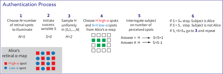
In Figure 3 we show how the authentication algorithm works. As mentioned above, the biometric device has stored Alice’s -map, so it can classify Alice’s retinal spots into high- spots, for which Alice has a high probability of seeing the light flash, and low- spots, for which this probability is low. The device chooses the number of spots it will illuminate (step 1). In the example of Figure 3, it is . The specific value of is the result of an optimization to be presented in the following.
We also define a success parameter , which is initiated at the value (step 2). Then, the device randomly selects a number (step 3), and illuminates spots of the type "high-" and spots of the type "low-" (step 4). In the example of Fig. 3, it is . The subject is then (step 5) interrogated on how many bright spots she perceived. If her answer equals , then we update the success parameter to , otherwise to . In the last step of the algorithm is compared with a positive upper value and with a negative lower value . If we stop the interrogation process, authenticating the subject as Alice. If , then we stop the process with a negative authentication, i.e. the subject is not Alice. Otherwise, we return to step 3 of the algorithm.
The choice of and depends on the desired values of and , as follows. Both Alice and Eve perform a random walk in -space with unit step and probabilities and , respectively, for a positive step, and and , respectively, for a negative step. If by we denote the interrogation round in which first reaches , then Norris the probability that Eve’s success parameter reaches the value and thus Eve is falsely identified as Alice is
| (5) |
Thus Eq. (5) is the probability that Eve will reach the value expected for Alice’s authentication before reaching the value expected for Alice’s non-authentication. To ensure that this probability is smaller than the specified tolerance , we may choose to be
| (6) |
where stands for the smallest integer greater than or equal .
Similarly, the probability that Alice’s parameter drifts to the low value , and thus Alice is falsely not authenticated, is equal to
| (7) |
To ensure that this probability is smaller than the specified tolerance , we may choose
| (8) |
where stands for the greatest integer not exceeding .
IV Quantum advantage using quantum light
We are now in position to explore the quantum advantage brought about by quantum light, in particular a single-photon source. Since the temporal summation window Holmes of the visual system is on the order of , we can use a single-photon source, for example a heralded single-photon source herald1; herald2; herald3; herald4, to produce a maximum of photons within a time interval , i.e. we need a production rate of at most 1 kHz, which is readily feasible. In the ideal case, the probability distribution of the number of photons incident on the cornea will be .
It is known, however, that optical losses degrade the sub-Poissonian statistics of quantum light. Hence, if a pulse of light containing exactly photons propagates inside the lossy material of the eye, the statistics of the number of detected photons will not be a spiked distribution like , but a broader distribution. Since the optical losses quantified by the parameter are not insignificant, the distribution of the detected photon number is not very far from the case of coherent light discussed previously. Yet, we will show that single photons do enhance performance, which demonstrates that quantum light sources can indeed be useful in addressing human vision.
In particular, for an optical loss parameter and exactly photons incident on the cornea, the distribution of the photon number after propagation through the lossy material is binomial with parameters , i.e.
| (9) |
whereas, using Eq. 1, the corresponding distribution for coherent light is a Poissonian with parameter , i.e.
| (10) |
where in this case is the mean incident number of photons per pulse. Note that in both cases the mean number of detected photons equals . However, the variance of this quantity with coherent light is , whereas the variance with quantum light is . In Fig. 4a we show an example of the slight difference of the two distributions, Eqs. (9) and (10), for and photons.

Now, the probability that Alice fails to perceive an illuminated high- spot is
| (11) |
whereas the probability that Alice does perceive an illuminated low- spot is
| (12) |
In these expressions the probability mass function is equal to either of Equation (9) for quantum light, or to of Equation (10) for laser light. The parameter enters Eq. (4), giving the probability that Alice succeeds in one particular interrogation. An example of the dependence of the parameter on the incident mean photon number is shown in Figure 4b. It is seen that is minimized at for laser light and for single photons, the minimum being and , respectively (Note that for a coherent state relevant to laser light is a continuous variable).
IV.1 Interrogation time
Having found Alice’s parameter for a given set of values and , we can use Eq. (4) to determine the mean number, , of interrogations required for Alice’s authentication, and choose to minimize . Indeed, by Theorem 1.3.5 in Norris we find
| (13) |
where the second term in the exact expression for was neglected as it is proportional to , and where is given by (6), is given by (8), and is given by (4). In Figure 4c we plot versus the number of illuminated retinal spots (pixels) for the two cases we consider, i.e. laser light and single-photons. It is seen that for laser light the optimal number of expected interrogations is , with the optimal number of spots being . For single-photons we find an optimal of approximately 23 expected interrogations with illuminated spots, i.e. we gain about 11.4% in interrogation time.
Finally, if we consider photon number as a resource, the fact that the optimal photon number per pulse for quantum light () is somewhat smaller than the corresponding number for laser light (), pushes the total advantage to 13.3%.
V Discussion
We have here presented an intuitive biometric authentication process using the human visual system’s ability to perform photon counting. The process rests on the perception of a number of illuminated spots on the retina. The performance of the authentication process in terms of false positive and false negative probability, as well as the interrogation time required to realize those two probabilities, is determined by the photon statistics of the stimulus light. We have shown that a single-photon source provides an advantage, even though the optical losses, which form the biometric fingerprint, degrade the sub-Poissonian statistics of the quantum stimulus light. Two comments are to be made. First, one might claim that the quantum advantage is small. However, a significantly larger quantum advantage cannot be excluded. This is because it is not straightforward to find the ultimate quantum limit of the general methodology, independent of the specific authentication strategy. Indeed, since the visual perception involves a number of nonlinearities, one might expect to be able to enhance the small difference in photon statistics between laser light and quantum light (at the photon detection level discussed previously) by designing another interrogation strategy. In the same context, one might argue that despite the quantum advantage shown here, the number of required interrogations is anyhow large. This is the reason we previously Loulakis devised an authentication strategy based on pattern recognition. This strategy led to a much faster authentication time with the same performance metrics. However, this strategy depends on further assumptions on the workings of visual perception and pattern recognition. In contrast, with the simple strategy considered herein we aimed at a straightforward to understand and analytically tractable demonstration of the promise of quantum light sources for studying the human visual system in general, and our biometric authentication methodology in particular. *
Appendix A
The proof of the Lemma is as follows.
| (14) |
For a set of odd cardinality and median , and for , we define
| (15) |
and . It is immediate that if , then . On the other hand, there are precisely sets with median and cardinality , since there are ways to choose the elements of in and ways to choose the elements of in . Hence, with it is
| (16) |
We can straightforwardly compute
| (17) |
For , we have
| (18) |
If then
where . Hence,
Likewise,
| (19) |
and
We may now substitute the preceding relations in (18) to get the recursive equation
In view of the initial condition (17), the assertion of the Lemma can now be proved inductively, or simply by noting that depends on only through and setting in equation (A).
Acknowledgements.
This work has been co-financed by the European Union and Greek national funds through the Operational Program Competitiveness, Entrepreneurship and Innovation, under the call "RESEARCH-CREATE- INNOVATE", with project title "Photonic analysis of the retina’s biometric photo-absorption" (project code: T1EDK-04921).Data Availability Statement
Data available on request from the authors.
References
References
- (1) J. A. Unar, W. C. Seng, and A. Abbasi, Pattern Recognit. 47, 2673 (2014).
- (2) W. Yang, S. Wang, N. M. Sahri, N. M. Karie, M. Ahmed, and C. Valli, Sensors 21, 6163 (2021).
- (3) N. Gisin, G. Ribordy, W. Tittel, and H. Zbinden, Rev. Mod. Phys. 74, 145 (2002).
- (4) S. Pirandola et al., Adv. Opt. Phot. 12, 1012 (2019). ;
- (5) M. Loulakis, G. Blatsios, C. S. Vrettou, and I. K. Kominis, Phys. Rev. Applied 8, 044012 (2017).
- (6) P. Sekatski, N. Brunner, C. Branciard, N. Gisin and C. Simon, Phys. Rev. Lett. 103, 113601 (2009).
- (7) N. Brunner, C. Branciard and N. Gisin, Phys. Rev. A 78, 052110 (2008).
- (8) F. Lucas and K. Hornberger, Phys. Rev. Lett. 113, 058301 (2014).
- (9) R. Pizzi, R. Wang and D. Rossetti, PLoS ONE 11, e0147464 (2016).
- (10) A. Dodel, A. Mayinda, E. Oudot, A. Martin, P. Sekatski, J.-D. Bancal, and N. Sangouard, Quantum 1, 7 (2017).
- (11) A. Pedram, Ö. E. Müstecaplıoğlu, and I. K. Kominis, arXiv:2111.03285v1.
- (12) S. Hecht, S. Shlaer, and M. H. Pirenne, J. Gen. Phys. 25, 819 (1942).
- (13) W. Bialek, Biophysics (Princeton University Press, 2012).
- (14) J. N. Tinsley, M. I. Molodtsov, R. Prevedel, D. Wartmann, J. Espigulé-Pons, M. Lauwers and A. Vaziri, Nature Comm.7, 12172 (2016).
- (15) M. Fox, Quantum Optics (Oxford University Press, 2006).
- (16) D. A. Baylor, T. D. Lamb and K.-W. Yau, J. Physiol. 288, 613 (1979).
- (17) F. Rieke and D. A. Baylor, Biophys. J. 71, 2553 (1996).
- (18) F. Rieke and D. A. Baylor, Biophys. J. 75, 1836 (1998).
- (19) F. Rieke and D. A. Baylor, Rev. Mod. Phys. 70, 1027 (1998).
- (20) N. Sim, D. Bessarab, C. M. Jones and L. A. Krivitsky, Biomed. Opt. Expr. 2, 2926 (2011).
- (21) N. Sim, M. F. Cheng, D. Bessarab, C. M. Jones and L. A. Krivitsky, Phys. Rev. Lett. 109, 113601 (2012).
- (22) N. M. Phan, M. F. Cheng, D. A. Bessarab and L. A. Krivitsky, Phys. Rev. Lett. 112, 213601 (2014).
- (23) P. C. Nelson, Phys. Biol. 13, 025001 (2016).
- (24) R. Holmes, M. Victora, R. F. Wang, and P. G. Kwiat, Vis. Res. 140, 33 (2017).
- (25) J. R. Norris, Markov Chains (Cambridge University Press, 1998)
- (26) M. Oxborrow, and A. G. Sinclair, Contemp. Phys. 46, 173 (2005).
- (27) G. S. Buller, and R. J. Collins, Meas. Sci. Tech 21, 012002 (2010).
- (28) M. D. Eisaman, J. Fan, A. Migdall, and S. V. Polyakov, Rev. Sci. Inst. 82, 071101 (2011).
- (29) E. Meyer-Scott, C. Silberhorn, and A. Migdall, Rev. Sci. Inst. 91, 041101 (2020).