Bifurcated symmetry breaking in scalar-tensor gravity
M. Yoshimura
Research Institute for Interdisciplinary Science, Okayama University
Tsushima-naka 3-1-1 Kita-ku Okayama 700-8530 Japan
ABSTRACT
We present models that simultaneously predict presence of dark energy and cold dark matter along with slow-roll inflation. The dark energy density is found to be of order , and the mass of dark matter constituent is meV. These numbers are given in terms of the present value of Hubble constant and the Plank energy : they are for the energy density and for the dark matter constituent mass. The basic framework is a multi-scalar tensor gravity with non-trivial conformal coupling to the Ricci scalar curvature in the lagrangian density. The key for a right amount of dark energy is to incorporate in a novel way the spatially homogeneous kinetic contribution of Nambu-Goldstone modes in a spontaneously broken multi-scalar field sector. Proposed theories are made consistent with general relativity tests at small cosmological distances, yet are different from general relativity at cosmological scales. Dark matter is generated as spatially inhomogeneous component of the scalar system, with roughly comparable amount to the dark energy. In some presented models a cosmological bifurcation of symmetry breaking of scalar sector is triggered by the spontaneous breaking of electroweak SU(2) U(1) gauge symmetry, hence the separation occurring simultaneously at the electroweak phase transition. The best experimental method to test presented models is to search for the fifth-force type of scalar exchange interaction with a force range, cm, whose coupling to matter is basically of gravitational strength.
Keywords Dark energy, Dark matter, Slow-roll inflation, Scalar-tensor gravity, Fifth force, Electroweak phase transition
1 Introduction
General relativity (GR for brevity) is a remarkable success as theory of gravity, passing all stringent tests in the solar system, merging binary pulser and gravitational wave detection [1], [2], [3]. Nevertheless, inflation that solves cosmological conundrums [4] requires a scalar degree of freedom [5], [6], and with introduction of conformal coupling the scalar degree of freedom inevitably links to the gravitational tensor field. Dark energy may also be related to existence of a scalar field [7], [8].
An interesting precursor of scalar-tensor gravity is Jordan-Brans-Dicke (JBD) theory [9], [10] which however failed in many ways, and one of the reasons may be traced to absence of scalar potential. Scalar-tensor gravity with potential term incorporated led to a plethora of models which attempt to solve the dark energy problem. All models of scalar-tensor gravity must clear classical and new tests of general relativity, which turns out non-trivial in many proposed models.
In the present work we propose the idea of using, in a novel way, Nambu-Goldstone modes of spontaneously broken symmetry in multi-scalar tensor gravity. When kinetic contribution of these modes is incorporated as a part of effective scalar potential, it gives rise to a new type of repulsive forces dependent on the metric determinant. The scalar fields in cosmology may generate both spatially homogeneous and and inhomogeneous components. We show that the spatially homogeneous part behaves as dark energy, with its equation of state factor -1, and the spatially inhomogeneous part behaves as dark matter, with its number energy density decreasing inversely proportional to the volume factor with cosmological evolution. Their predicted energy densities at the present epoch are of order (with eV the Hubble energy and eV the Planck energy in our definition). Mass of dark matter constituent is of order a few meV, hence all energy scales are given by this combination of Hubble and Planck energies. Bifurcation of dark matter from dark energy may be triggered by the electroweak SU(2) U(1) gauge symmetry breaking. Another great merit of Nambu-Goldstone modes is that they clear GR tests in a trivial way.
The present paper is organized as follows. In Section 2 we lay out our theoretical framework of scalar-tensor gravity based on conformal coupling of multi-scalar sector to the massless graviton. The scalar system is assumed to have a continuous global symmetry, and role of Nambu-Goldstone modes is emphasized to produce the new type of repulsive forces. In Section 3 we discuss cosmology of symmetric scalar-tensor gravity, taking as an example the simplest O(2) model made of two real scalar fields, and show that slow-roll inflation and late time accelerating universe are both realized by a modest choice of parameter range. Tracker solution at late times, recognized as spatially uniform, predicts a right amount of dark energy density given by 1.7 meV independent of model parameters. Spatially inhomogeneous components are identified in the linearized approximation around homogeneous solutions, and are decomposed in terms of their wave vectors, and each component is recognized as dark matter of definite momentum, with its number density being inversely proportional to the volume factor. Section 4 is devoted to explanation of the bifurcated symmetry breaking triggered by the electroweak gauge symmetry breakdown. Two possibilities exist depending on whether the scalar field has SU(2) U(1) quantum numbers or not. It is found that dark scalars in viable models should have no SU(2) U(1) quantum number. In Section 5 we present some rudimentary ideas on how this class of models may be tested experimentally in laboratories on earth. The paper ends with a brief summary.
We use the natural unit of and the unit Boltzmann constant throughout the present work unless otherwise stated.
2 Theoretical framework
We consider a class of local field theory in four space-time dimensions of the following type:
| (1) |
written in terms of graviton metric field , a number of scalar fields , and standard model fields generically denoted by , and . Our signature convention of flat metric is ), and the metric determinant . The constant is our squared Planck energy. The scalar potential and the conformal coupling function are assumed to have a global symmetry, the simplest case being a function of field modulus, , for real scalars which gives symmetry. With a constant the theory is a trivial extension of standard particle theory, and can realize inflation taking an appropriate form of potential . We introduce here a non-trivial function , and this function may be expanded in terms of dimensionless field .
The metric frame thus introduced may be called JBD frame. It is often more convenient to introduce the Einstein frame by a Weyl rescaling, ,
| (2) |
We denote hereafter the new metric by . A simple conformal factor and potential of the form is considered in the present work;
| (3) | |||
| (4) |
The potential of scalar system exhibits a spontaneous symmetry breaking due to a negative curvature at the origin . Our model is characterized by two dimensionless parameters, , taken to be of order unity, and other parameters of non-vanishing mass dimensions. The constant is later adjusted by requirement of vanishing cosmological constant. The mass value (taken positive) is left arbitrary for the moment. More complicated generalization of potential and conformal factor is possible, but this simplest case is sufficient to explain main features of our theory.
Scalar kinetic term can be recast to the standard form by a change of field normalization. First, we separate modulus part and angular part by introducing orthogonal transformation , which transforms a reference vector, say , to general -vector . Then, the kinetic term is written, using ,
| (5) |
The second term written in terms of derivatives of orthogonal matrix elements is contribution from Nambu-Goldstone modes, since the potential does not depend on Nambu-Goldstone angular mode variables that appear in . In the simplest O(2) case this term is when . In O(3) case kinetic Goldstone term is using the standard angular variables, . In both cases they are written in terms of generalized angular momentum operator with . In cosmology is practically time derivative.
Except Nambu-Goldstone kinetic terms, one can change scalar field variables to the standard form;
| (6) | |||
| (7) | |||
| (8) |
For the choice of eqs.(3), (4), these are explicitly
| (9) | |||
| (10) |
This has a limiting behavior at , (assuming and neglecting terms)
| (11) |
Nambu-Goldstone modes appear only in kinetic terms of lagrangian. The field equation for O(2) Nambu-Goldstone mode is , to give its generic solution,
| (12) |
with a constant of integration giving the value of angular momentum operator. One may define an effective potential, adding a centrifugal term; in the small field limit,
| (13) |
The centrifugal term changes location of potential minimum (at without centrifugal term). Except in inflationary epoch this potential formula and its extensions in the low energy limit are adequate in our discussion.
Nambu-Goldstone kinetic terms in extended models may emerge in a far more non-trivial way. Suppose, taking a real component model, that two parts of and components separately appear with two different integration constants,
| (14) |
giving different centrifugal repulsions. This occurs when the scalar system has spontaneously a broken O() O() symmetry. We later encounter an example of . This is a bifurcation of symmetry breaking in the dark sector, and provides a separation mechanism of dark energy in the dark sector.
We note in passing that there exist stringent constraints from GR tests imposed on an interesting model of restored discrete symmetry [11], although the necessary Vainshtein decoupling [12] around a massive astronomical body is realized in this and related models. Historically, the Vainshtein decoupling played an important role in the massless limit of massive spin 2 graviton theory. Two degrees of freedom associated with the massless graviton decouples from the rest of three degrees of freedom within what is called Vainshtein radius around a massive astronomical object, becoming of order cm (roughly the size of presently observable universe) for the sun and a graviton mass of order the Hubble constant eV. (This radius changes as with the graviton mass .)
A different decoupling mechanism works in our scalar-tensor gravity due to centrifugal repulsive potential of Nambu-Goldstone modes, which is a key in passing GR tests at smaller distances.
3 Cosmology
We first discuss cosmology in O(2) symmetric scalar-tensor theory. O() symmetry extension is straightforward. The spatially flat Robertson-Walker metric [4] given by is sufficient for our discussion. In the flat spacetime the absolute value of scale factor may be taken arbitrarily, and we choose the normalized scale factor such that the present scale factor is unity: . The Nambu-Goldstone field equation is
| (15) |
which makes it possible to incorporate in the lagrangian density for scalar field a centrifugal term, to give an effective potential ,
| (16) |
with an integration constant. is related to the Hubble constant when we discuss late time solution. The Einstein and scalar field equations are then
| (17) | |||
| (18) | |||
| (19) |
dot being time derivative. We assume for this discussion as if a non-vanishing existed since a pre-inflation epoch. But at inflationary epoch and also in subsequent radiation-dominated epoch the centrifugal term is not important, and its importance becomes evident at late epoch of accelerating universe. For radiation and matter energy density we only need to know that in radiation dominated epoch (also ), while in matter dominated epoch.
We fine tune the cosmological constant such that (the second term arising from the zero field limit of term in eq.(10)). It is suitable to use dimensionless Planckian time unit and rewrite gravitational and field equations:
| (20) | |||
| (21) | |||
| (22) | |||
| (23) |
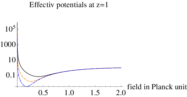
The dimensionless effective potential, of eq.(21), near the present cosmological epoch at a redshift 1 or (in our normalized unit) is illustrated in Fig(1), although the chosen parameters (for a less computer tension) are not appropriate for a realistic choice. Nonetheless, solutions derived from differential equations for graviton and scalar field exhibit a rich variety of interesting behaviors. Thus, this model is capable of solving cosmological conundrums both at inflation and at late times.
3.1 Inflationary epoch ending at thermalized hot universe
Inflation in the usual picture occurs when the potential dominates over kinetic term, . Suppose that a large field , or , exists in a pre-inflationary epoch, presumably due to fluctuation of quantum gravity effects. The slow-roll inflation [5], [6], [4] is realized under the two conditions, and (the prime ′ indicating field derivative), which read in our model as
| (24) |
We expect that inflation ends at .
With , the first condition of eq.(24) turns out more stringent than the second, and one derives a sufficient condition, which becomes a condition for initial values of , assuming tracker solution later derived (see of eq.() ),
| (25) |
This is a condition readily satisfied, for instance by taking .
We illustrate in Fig(2) a toy model example of time evolution. Initial condition for numerical simulations has been determined by seeking initial values when one imposes and .

Thermalized universe is expected to emerge using production mechanism of standard model particles as outlined in [13], [14]. Rapidly oscillating scalar field at the end of inflation gives rise to copious Higgs boson production through coupling to standard model Higgs boson of the form, . Non-perturbative parametric amplification of Floquet-type is responsible for this mechanism. Thermal energy of produced Higgs pairs is then converted to other relativistic particles, which achieves radiation dominated universe.
3.2 Epoch of accelerating universe again
Energy density of thermalized relativistic and non-relativistic particles changes with cosmic scale factor as and , hence radiation-dominated universe appears at earlier epoch and then matter dominated-universe follows. Dark energy density does not change with expansion, and the universe at later epoch may enter into dark energy dominated universe governed by the scalar field. Note that the settled potential minimum at the end of inflation differs from the true minimum at later epochs, and this mismatch accelerates the late time universe.
Detailed scalar dynamics at redshift is analyzed by solving the equation,
| (26) | |||
| (27) |
where the dark matter energy density is estimated as , from the present observed value.
We shall search solutions in which matter contribution is negligible. Assuming a small , we seek a solution in which two terms, quartic field term and centrifugal repulsion, nearly balance. This gives
| (28) |
Inserting this relation into the Einstein equation, one derives
| (29) |
Under the condition , the solution is given by
| (30) |
The present Hubble constant is defined by , which determines ; . From observational values one may estimate years (taking ) compared to years. In order to determine , we go back to the Einstein equation, which reads as
| (31) |
Thus,
| (32) |
The equation of state factor is defined by
| (33) |
and is found to be nearly , because the ratio
| (34) |
is small with for the solution we found. We call this solution the tracker solution.
The dark energy density is independent of unknown couplings of the model, and is given by
| (35) |
This is a prediction of tracker solution for a single Goldstone mode. Its value can be raised to times this value when there exist Goldstone modes.
To check how this solution is good, we analyze the linearized equation around this solution. In terms of , the linearized equation is
| (36) |
We have numerically integrated this equation in a time range , and found that . Hence deviation from the tracker solution is a minor correction.
We now analyze spatially inhomogeneous contribution of scalar field by working out linearized field equation around the tracker solution. Differential equations to be solved are
| (37) |
Coefficient of right hand side is calculated as
| (38) |
at the present epoch .
The emerging picture of this simplest two-component O(2) model is that Nambu-Goldstone centrifugal repulsion gives rise to a homogeneous dark energy with its energy density of order , while inhomogeneous part provides dark matter of mass .
4 Extension for bifurcated symmetry breaking
4.1 Trigger by spontaneous electroweak symmetry breaking
There is no reason the scalar sector is not linked to the Higgs doublet present in SU(2) U(1) electroweak theory spontaneously broken down to UEM(1). There are two possibilities, depending on whether dark scalars have SU(2) U(1) quantum numbers or not.
We first discuss the case of dark scalar being a SU(2) U(1) singlet. In this subsection we neglect temperature effects, and concentrate on tracker solutions at temperatures much below the electroweak phase transition. In the next subsection we consider the region around the electroweak critical temperature. The potential part of fundamental lagrangian is given by
| (39) |
with using real fields . By a SU(2) U(1) transformation one can take homogeneous fields parallel to . The effective Higgs-scalar potential is given by
| (40) |
It would be conceptually simpler to think of a O(N-1) broken scheme in which the potential has a form of linear combinations among with different coefficients. The potential given by eq.(40) is a special combination of minimal different coefficients. It turns out that this simplified form is sufficient for our purpose.
Potential minimum is determined by solving algebraic equations for ,
| (41) | |||
| (42) |
Assuming a small , an interesting tracker solution satisfies
| (43) |
The effective potential after eliminating is given by
| (44) | |||
| (45) |
An interesting case is given when two terms cancels such that under the condition . The tracker solution in this case is
| (46) | |||
| (47) |
Mass squared matrix for dark matter fields is given by
This model describes a dark matter mass much closer to standard particle physics, of order a few meV.
The full set of non-linear coupled equation using dimensionless fields and is given by
| (53) | |||
| (54) | |||
| (55) | |||
| (56) |

4.2 Bifurcation at electroweak critical temperature
One has to incorporate effects of high temperature in the early universe. We are particularly interested in behaviors of order parameters, around the electroweak phase transition at temperature (electroweak critical temperature). The effective potential is now replaced by the Gibbs free energy, and one has a finite temperature contribution to field squared term of the form, , with a dimensionless constant of order unity. We keep using the terminology of effective potential instead of the Gibbs free energy, to write it as
| (57) |
There is no temperature dependent correction related to scalar field due to their extremely feeble interaction of gravitational strength with ambient particles.
The equation that determines stationary points is modified by temperature dependent term; below stationary points are determined by
| (58) | |||
| (59) |
with . The obvious constraint gives a condition;
| (60) |
As , . Thus, we establish that both of vanish above the critical temperature, and the electroweak critical temperature is the point of bifurcation of dark scalar fields. From a consistency of the above equation we conclude that also approaches to zero at the critical temperature,
| (61) |
4.3 Doublet case is not viable
We have also considered the case of dark scalars being SU(2) U(1) doublet. Both complex SU(2) doublets may be described by four real fields, ,
We take an extended SU(2) U(1) symmetric potential replacing the usual Higgs potential by
| (67) |
with all taken positive.
We studied this model in great detail, but the bottom line is existence of stable charged scalars of masses, (a few meV). The charged scalars have electromagnetic interaction, and their pair production via analogue of Bethe-Heitler pair production for is our concern. Cross section is lots larger by the factor than Bethe-Heitler process, and it drastically modifies the behavior of electromagnetic showers above the shielding energy keV. We believe that this is sufficient to reject the doublet case.
5 Coupling of neutral dark scalar to matter and laboratory test
An attractive feature of presented models is the uniqueness of coupling to standard theory particles: the new degree of scalar field couples to standard particles by the conformal factor in the Einstein frame lagrangian, and in the field equation. This coupling is related to cosmological evolution of scalar fields via varying , giving prediction of testable consequences.
First of all, the tracker solution at recent epochs predicts variation of basic coupling constants. For the fine structure constant, its fractional variation is found to be of order divided by the age of universe in both viable models of Section 3 and Section 4. For instance, in genetic model of Section 3 it is given by
| (68) |
which is utterly impossible to detect.
For discussion of model tests in laboratories on earth we recapitulate in the following table results on dark energy density, masses of linearized quanta, and their coupling to standard model particles as defined by the coefficient of , which was obtained in the preceding section. The required minimal number of parameters, hence the most predictive results are assumed in the table, hence these numbers are only a guide ignoring more complexities.
| Models | Dark energy density | Dark quantum mass | Coupling to standard particles |
|---|---|---|---|
| O(2) | |||
| SU(2) U(1) singlet bifurcation |
We have studied possibilities for dark quantum search in table-top atomic experiments using coherence, but have found no good method. The best experimental method seems to be the classical approach of the firth-force search such as refined torsion balance experiments. If one could focus on the force range of scalar mediated interaction, (0.1) mm, corresponding to a few meV mass, in these experiments, the method may become ideal.
6 Summary
The multi-scalar field is a key for realization of slow-roll inflation and accelerating universe at late times. Conformal coupling to the scalar curvature in lagrangian provides to angular Nambu-Goldstone modes a centrifugal repulsive potential, a positive constant times where is the modulus of scalar field. This repulsive force shifts potential minimum location with cosmological evolution, otherwise fixed by an original fundamental lagrangian. Resulting tracker solution recognized as spatially homogeneous component follows a time varying potential minimum at late times, and gives rise to dark energy density of order (a few meV)4, with the equation of state factor -1. On the other hand, the spatially inhomogeneous component gives a dark matter candidate, its number density being inversely proportional to the volume factor, third power of cosmic scale factor. The scalar boson mass is predicted to be an order unity coupling constant times meV.
We further proposed a mechanism of bifurcated symmetry breaking triggered by the electroweak SU(2) U(1) gauge symmetry breaking. It was found that viable models preclude SU(2) U(1) quantum numbers for dark scalar. Nambu-Goldstone modes emerge as a result of bifurcation of symmetry breaking.
All models discussed in the present work pass tests of general relativity at small cosmological distances, yet it deviates from general relativity at cosmological scales. Experimental method to search for dark matter quantum in laboratories on earth has also been discussed. Considering cm range corresponding to 1 meV, search for the fifth-force type interaction of gravitational strength may be promising.
Acknowledgements
This research was partially supported by Grant-in-Aid 21K03575 from the Japanese Ministry of Education, Culture, Sports, Science, and Technology.
References
- [1] C.M. Will, The Confrontation between General Relativity and Experiment, arXiv:gr-qc/0103036v1 (2002).
- [2] B. P. Abbott et al. Phys.Rev.Lett. 116, 221101 (2016). Post-Newtonian GR tests of discovered gravitational wave are given with no indication of deviation from GR, and a graviton mass limit is given; cm roughly corresponding to length, 1 pc/3, or eV.
- [3] B. P. Abbott et al. Phys.Rev.Lett. 119, 161101 (2017). LIGO Scientific Collaboration and Virgo Collaboration, Fermi Gamma-ray Burst Monitor, and INTEGRAL, Astrophy. Journal Lett. L13, 848 (2017). It was pointed out by many that this event of simultaneous observation of gravitational wave and electromagnetic wave originating from binary neutron star merger constrains certain class of scalar-tensor gravity. Our model does not belong to this class.
- [4] A standard textbook of modern cosmology is S. Weinberg, Cosmology, Oxford University Press, New York (2008).
- [5] A. Linde, Phys. Lett. B108, 389 (1982); B114, 431 (1982).
- [6] A. Albrecht and P. Steinhardt, Phys.Rev.Lett. 48, 1220(1982).
- [7] B. Ratra and P.J.E. Peebles, Phys.Rev.D37, 3406 (1988).
- [8] C. Wetterich, Nucl. Phys. B302, 668 (1988). Astron. Astrophysics, 301, 32 (1995).
- [9] P. Jordan, Z. Phys. 157, 112 (1959).
- [10] C. Brans and H. Dicke, Phys. Rev. 124, 925(1961).
- [11] The idea of using a restored spontaneously broken symmetry is traced back to a model of discrete reflection symmetry; K. Hinterbichler and J. Khoury, Phys. Rev. Lett. 104 , 231301 (2010). Our model introduces restoration of continuously broken theory, which brings out Nambu-Goldstone modes, a crucial element for a new type of scalar-tensor gravity.
- [12] A.I. Vainshtein, Phys. Lett. 39B, 393 (1972),
- [13] M. Yoshimura, Prog. Theor. Phys. 94, 873(1995).
- [14] L. Kofman, A. Linde, and A.A. Starobinsky, Phys. Rev. Lett. 73, 3195(1994).
- [15] R. Cameron et al, Phys.Rev. D47, 3707 (1993).
- [16] P. Pugnat et al., Phys. Rev. 78, 092003 (2008).