Learning Swarm Interaction Dynamics from Density Evolution

Christos N. Mavridis Amoolya Tirumalai John S. Baras Thanks: This work was supported in part by the Defense Advanced Research Projects Agency (DARPA) under Agreement No. HR00111990027 and by ONR grant N00014-17-1-2622. Thanks: The authors are with the Department of Electrical and Computer Engineering and the Institute for Systems Research, University of Maryland, College Park, MD 20742 USA (e-mails: mavridis@umd.edu, ast256@umd.edu, baras@umd.edu).

Abstract

We consider the problem of understanding the coordinated movements of biological or artificial swarms. In this regard, we propose a learning scheme to estimate the coordination laws of the interacting agents from observations of the swarm’s density over time. We describe the dynamics of the swarm based on pairwise interactions according to a Cucker-Smale flocking model, and express the swarm’s density evolution as the solution to a system of mean-field hydrodynamic equations. We propose a new family of parametric functions to model the pairwise interactions, which allows for the mean-field macroscopic system of integro-differential equations to be efficiently solved as an augmented system of PDEs. Finally, we incorporate the augmented system in an iterative optimization scheme to learn the dynamics of the interacting agents from observations of the swarm’s density evolution over time. The results of this work can offer an alternative approach to study how animal flocks coordinate, create new control schemes for large networked systems, and serve as a central part of defense mechanisms against adversarial drone attacks.

Index Terms:

Learning, Networks of autonomous agents, Biological Networks, Swarm interaction dynamics.

I Introduction

The highly coordinated movements of animal flocks are among the most fascinating phenomena to be found in nature, and understanding their dynamics and coordination laws has been the research focus for many scientists over the last decades [1, 2, 3, 4, 5, 6].

Extracting the laws of interaction between agents of general networked systems finds applications in a wide range of fields, from power systems and chemical reaction networks, to social networks and UAV swarms [4, 5, 7, 3, 8, 9]. Statistical [10], and model-based [2, 3, 7, 11] learning approaches have been used to learn the interaction rules between agents. There are generally two broad approaches in modeling the underlying dynamics of ensembles of self-organizing agents: the microscopic particle models, described by ordinary or stochastic differential equations, and the macroscopic continuum models, described by partial differential equations (PDEs). Agent-based models assume behavioral rules at the individual level, such as velocity alignment, attraction, and repulsion [2, 3, 4, 5], while macroscopic models, consider large number of interacting agents, approaching the mean-field limit. These models typically consist of hydrodynamic PDEs defined on macroscopic quantities, such as the swarm’s density [12, 13, 14], and have been studied for the analysis and control of artificial swarms, mainly in robotic applications [15, 16, 17].

Particle models have been mainly used in numerical simulations and learning methodologies [7, 18, 11]. Recently, Mao et al. in [11] modeled the interactions with respect to a fractional differential system of equations, and Matei et al. in [7] proposed an energy-based approach by modeling the network as a port-Hamiltonian system [19]. However, useful real-life data of particle trajectories are difficult to extract and may require substantial memory and computation resources [5, 9]. The experimental measurements, which usually involve digital imaging or high-resolution GPS devices, are difficult to acquire and are subject to artificially created noise originating from both the sensors and the processing algorithms. In [5], for example, stereometric and computer vision techniques have been used to measure long-time and long-distance 3D position trajectories of starling flocks, and in [9], GPS devices were installed to homing pigeons flying in small flocks of no more than 13 individuals.

On the other hand, useful approximations of the ensemble’s density evolution can be easier to extract, often by applying simple morphological operators on vision-based recordings. For this reason, we believe that developing learning algorithms based on the macroscopic quantities can play a crucial role in the analysis of collective motion, and only remains inhibited due to computational expense; the flocking dynamics can be non-local as well as nonlinear [13], which results in a costly computation of the solution of the corresponding hydrodynamic equations [11, 20].

Contribution. In this work, we introduce a modified Cucker-Smale model of non-local particle interaction for velocity consensus [3, 21] to efficiently solve the macroscopic hydrodynamic equations. We propose a family of parametric interaction functions which are shown to correspond to Green’s functions associated with an appropriately defined differential operator. This allows for the transformation of the macroscopic hydrodynamic integro-differential equations into an augmented system of PDEs, which, in turn, results in a speed-up in the computation of the non-local interaction terms. We investigate the conditions under which time-asymptotic flocking is achieved, and utilize the computational advantages of the proposed methodology to construct an iterative optimization algorithm to learn the interaction function based on observations of the particle density evolution. Finally, we also investigate the advantages of incorporating the proposed interaction function model in learning algorithms based on particle trajectories (microscopic models). The results of this work can be used to model and understand biological and artificial flocks with applications in the control of large networked systems and artificial robotic swarms, and in defensive mechanisms against adversarial swarm attacks.

II Mathematical Models and Notation

In this section we introduce the notation that will be followed throughout the manuscript, define time-asymptotic flocking and the Cucker-Smale particle dynamics, and derive the mean-field macroscopic equations.

II-A The Cucker-Smale Model

Consider an interacting system $\mathcal{G}$ of $N$ identical particles (representing autonomous agents) with unit mass in $\mathbb{R}^{d}$ , $d\in\{1,2,3\}$ . Let $x_{i}(t),\ v_{i}(t)\in\mathbb{R}^{d}$ represent the position and velocity of the $i^{th}$ -particle at each time $t\geq 0$ , respectively, for $1\leq i\leq N$ . Then the general Cucker-Smale system [3] is a dynamical system of $(2Nd)$ ODEs:

\begin{cases}\frac{dx_{i}}{dt}&=v_{i}\\ \frac{dv_{i}}{dt}&=\frac{1}{N}\sum_{j=1}^{N}\psi(x_{j},x_{i})(v_{j}-v_{i})\end{cases}

(1)

where $x_{i}(0)$ , and $v_{i}(0)$ are given for all $i=1,\ldots,N$ , and ${\psi:\mathbb{R}^{d}\times\mathbb{R}^{d}\rightarrow\mathbb{R}}$ represents the interaction function between each pair of particles. We define the center of mass system $(x_{c},v_{c})$ of $\mathcal{G}=\left\{(x_{i},v_{i})\right\}_{i=1}^{N}$ as

x_{c}=\frac{1}{N}\sum_{i=1}^{N}x_{i},\quad v_{c}=\frac{1}{N}\sum_{i=1}^{N}v_{i}

(2)

We are interested in symmetric interaction functions $\psi(x,s)=\psi(s,x)$ , in which case system (1) implies

\frac{dx_{c}}{dt}=v_{c},\quad\frac{dv_{c}}{dt}=0

(3)

which yields a unique solution

x_{c}(t)=x_{c}(0)+tv_{c}(0),\ t\geq 0

(4)

Under additional assumptions on $\psi$ (see Section III-A), system (1) can be shown to converge to a velocity consensus, while preserving spatial coherence, a property that is known as time-asymptotic flocking, defined as follows:

Definition 1 (Time-Asymptotic Flocking).

An $N-$ body interacting system $\mathcal{G}=\left\{(x_{i},v_{i})\right\}_{i=1}^{N}$ exhibits time-asymptotic flocking with bounded fluctuation if and only if the following two relations hold:

•

(Velocity alignment): The velocity fluctuations approach zero asymptotically, i.e.

$\lim_{t\rightarrow\infty}\sum_{i=1}^{N}\left\|v_{i}(t)-v_{c}(t)\right\|^{2}=0$
•

(Spatial coherence): The position fluctuations are uniformly bounded, i.e. for some $0<\Lambda<\infty$ ,

$\sup_{t\geq 0}\left\|x_{i}(t)-x_{c}(t)\right\|<\Lambda,\ \forall i\in\left\{1,\ldots,N\right\}$

Throughout this article, we will be investigating flocking behaviors and will be working with the fluctuation variables around the center of mass system, defined as:

(\hat{x}_{i},\hat{v}_{i}):=(x_{i}-x_{c},v_{i}-v_{c})

(5)

which can be shown to satisfy the same Cucker-Smale dynamics described in (1). We will take advantage of the spatial coherence of the flocking behavior, and define the position variables $\hat{x}_{i}$ in a compact support $D:=\left\{x\in\mathbb{R}^{d}:\|x\|<L/2\right\}$ for some finite $L>0$ and for all $i\in\left\{1,\ldots,N\right\}$ , with $\|\cdot\|$ representing the standard Euclidean norm in $\mathbb{R}^{d}$ .

The set $D$ is time-dependent and represents a subset of $\mathbb{R}^{d}$ centered at the center of mass of the swarm $x_{c}(t)$ , $t\geq 0$ , outside of which, the density of the swarm is considered negligible. We note that time-dependent transformation (5) only requires the knowledge of the initial conditions $x_{i}(0)$ and $v_{i}(0)$ , $i=1,\ldots,N$ .

II-B The Mean-Field Limit

When the number of agents $N$ becomes large, the use of continuum models for the evolution of a density of individuals becomes essential. In the following, we introduce a continuum model based on the hydrodynamic description derived by studying the mean-field particle limit following the Cucker-Smale model (1).

Consider the joint probability triple of the entire particle system $\{\Omega:=\mathbb{R}^{2Nd},\mathcal{B}(\Omega),P_{xv}\}$ , the state space for each particle $\{\mathbb{R}^{2d},\mathcal{B}(\mathbb{R}^{2d})\}$ and define the empirical (random) probability measure $F_{xv}^{N}:\Omega\times[t_{0},t_{f}]\times\mathcal{B}(\mathbb{R}^{2d})\rightarrow[0,1]$ such that

F_{xv}^{N}(t,A):=\frac{1}{N}\sum_{i=1}^{N}\mathbb{I}_{A}((x_{i}(t),v_{i}(t)))

(6)

where $\mathbb{I}_{A}(\cdot)$ is the indicator function, $A\in\mathcal{B}(\mathbb{R}^{2d})$ . Some authors use Dirac measures (not the Dirac delta function) in this definition. $F_{xv}^{N}$ is a random measure which is purely atomic. Using arguments originally due to McKean and Vlasov [22, 23], it can be shown that there exists a deterministic and continuous $F^{*}_{xv}$ such that $F_{xv}^{N}\overset{a.e.}{\to}F^{*}_{xv}$ in the weak sense, and, using Ito’s lemma, that the joint probability density $f^{*}_{xv}:[t_{0},t_{f}]\times\mathbb{R}^{2d}\rightarrow\mathbb{R}_{0}^{+}$ associated with this measure, evolves according to the forward Kolmogorov equation on $[t_{0},t_{f}]\times\mathbb{R}^{2d}$ :

\begin{cases}\partial_{t}f^{*}_{xv}+\nabla_{x}\cdot(vf^{*}_{xv})+\nabla_{v}\cdot(\mathcal{F}f^{*}_{xv})=0\\ \mathcal{F}(t,x,v):=\int_{\mathbb{R}^{2d}}\psi(x,s)(w-v)f^{*}_{xv}(t,s,w)dsdw.\end{cases}

(7)

We define the marginal probability density $\rho:[t_{0},t_{f}]\times D\rightarrow\mathbb{R}^{+}_{0}$ (henceforth referred to only as density) as

\rho(t,x):=\int_{\mathbb{R}^{d}}f^{*}_{xv}(t,x,v)dv

(8)

and the momentum density $m:[t_{0},t_{f}]\times D\rightarrow\mathbb{R}^{d}$ and bulk velocity $u:[t_{0},t_{f}]\times D\rightarrow\mathbb{R}^{d}$ as

m(t,x):=\int_{\mathbb{R}^{d}}vf^{*}_{xv}(t,x,v)dv:=\rho(t,x)u(t,x)

(9)

where $D\subseteq\mathbb{R}^{d}$ . It is additionally assumed that $\rho,m,u$ are compactly supported. Substituting in (7), we obtain the $(d+1)$ compressible Euler equations on $[t_{0},t_{f}]\times D$ (see also [12]):

\begin{cases}\partial_{t}{\rho}+\nabla_{x}\cdot m=0\\ \partial_{t}{m}+\nabla_{x}\cdot(\rho^{-1}mm^{T})=\rho\mathcal{L}_{\psi}m-m\mathcal{L}_{\psi}\rho\end{cases}

(10)

where

\mathcal{L}_{\psi}\phi(t,x)=\int_{D}\psi(x,s)\phi(t,s)ds.

(11)

is an integral transform with kernel $\psi:D\times D\rightarrow\mathbb{R}$ .

III Screened Poisson Mediated Flocking

The integral transforms in the right hand side of (10), which originate from the non-local interaction terms in the Cucker-Smale model, make the compressible Euler equations (10) a system of partial integro-differential equations, which is extremely challenging to solve. We approach the solution of system (10) by transforming it into an augmented system of PDEs, in order to use existing numerical methods to solve it.

Suppose that, by construction, the interaction function $\psi$ is a Green’s function associated with some linear partial differential operator $\mathcal{L}_{x}:L^{2}(D;\mathbb{R})\rightarrow L^{2}(D;\mathbb{R})$ , such that

\mathcal{L}_{x}y(t,x)=\phi(t,x)

(12)

implies

y(t,x)=\int_{D}\psi(x,s)\phi(t,s)ds.

(13)

Then, system (10) is equivalent with the augmented system of ( $2d+2$ ) partial differential equations:

\begin{cases}\partial_{t}{\rho}+\nabla_{x}\cdot m=0\\ \mathcal{L}_{x}z=\rho\\ \mathcal{L}_{x}y=m\\ \partial_{t}{m}+\nabla_{x}\cdot(\rho^{-1}mm^{T})=\rho y-zm.\end{cases}

(14)

For the global regularity of system (14) one can refer to [13] and the references therein. A classical example for $\mathcal{L}_{x}$ is the operator associated with the Poisson equation that arises in self-gravitational hydrodynamics [24]. However, in order to alleviate the computational bottleneck introduced by the non-local integral terms in (10), the operator $\mathcal{L}_{x}$ needs to be defined in a way such that:

$(a)$

the newly introduced subsystem

$\displaystyle\mathcal{L}_{x}z=\rho$

$\displaystyle\mathcal{L}_{x}y=m$

can be efficiently solved with numerical methods, which is the case, for example, if $\mathcal{L}_{x}$ is an elliptic operator,
$(b)$

the Green’s function $\psi$ defined in (13) retain the necessary properties of an interaction function that can drive the Cucker-Smale model (1) to asymptotic flocking behavior, and
$(c)$

$\mathcal{L}_{x}$ , and consequently $\psi$ , depend on a set of parameters that make $\psi$ appropriate to model different interaction function profiles, depending on the behavior of the swarm.

With this in mind, we propose $\mathcal{L}_{x}$ to be the parametrized screened Poisson partial differential operator

\mathcal{L}_{x}:=-\frac{1}{2k}(\partial_{x}^{2}-\lambda^{2})

(15)

defined in the domain $D:=\left\{x\in\mathbb{R}^{d}:\|x\|<L/2\right\}$ with homogeneous Dirichlet boundary conditions.

Remark 1.

We note that the choice of the proposed operator $\mathcal{L}_{x}$ in (15) is not necessarily unique. However, to our knowledge, there is no formal method to construct an operator $\mathcal{L}_{x}$ , and its associated Green’s function $\psi$ , that satisfy the conditions (a), (b), and (c) as described above.

To highlight the importance of conditions (a), (b), and (c), we stress that they allow for the system of partial integro-differential equations (10) to be solved faster, as an augmented system of PDEs. This is in contrast to the use of a standard kernel, e.g., the fractional Laplacian used in [11], that results in solving a system of fractional partial integro-differential equations. In the rest of this section, we will present an analysis of the proposed family of Green’s functions as interaction functions of a Cucker-Smale model (1), in the one-dimensional case ( $d=1$ ), which, in Section IV will be generalized to higher dimensions. When $d=1$ , system (14) can be compactly written as

\begin{cases}\partial_{t}U+\partial_{x}F(U)=S(Y,U)\\ \mathcal{L}_{x}Y=U\end{cases}

(16)

where $U:=[\rho,m]^{T}$ , $F:=[m,m^{2}\rho^{-1}]^{T}$ , $S:=[0,\rho y-zm]^{T}$ , and $Y:=[z,y]^{T}$ . The Green’s function $\psi$ associated with the BVP introduced in (15) can be analytically computed as (see Appendix A):

\psi(x,s)=\begin{cases}K\sigma_{p}(s)\sigma_{m}(x)&s\leq x\\ K\sigma_{m}(s)\sigma_{p}(x)&s>x\end{cases}

(17)

where

$\displaystyle K$	$\displaystyle=-\frac{k}{\lambda}\frac{1}{e^{\lambda L}-e^{-\lambda L}}$	(18)
$\displaystyle\sigma_{p}(z)$	$\displaystyle=2\sinh\left(\lambda(z+L/2)\right)$
$\displaystyle\sigma_{m}(z)$	$\displaystyle=2\sinh\left(\lambda(z-L/2)\right)$

One of the parameters of the interaction function $\psi$ in (17), which affects the flocking behavior of the system $\mathcal{G}$ , is the size $L$ of the bounded domain $D$ in which it is defined. The effect of the boundedness of the domain is illustrated in Fig. 1, where, for different fixed values of $x$ , $\psi(x,s)$ is compared to the function

\hat{\psi}(x,s)=\frac{k}{\lambda}e^{-\lambda\|x-s\|}

(19)

which is the Green’s function corresponding to $\mathcal{L}_{x}$ defined in an infinite domain. We can interpret this effect as a tendency to avoid the spread of the swarm in large distances with respect to the swarm’s center of mass at each time step.

Refer to caption — Fig. 1: (left) Illustration of $\psi(x,\cdot)$ (17) for different values of $x$ , and for $\lambda=1$ , $k=4$ on $[-\pi,\pi]$ . The function $\hat{\psi}(x,s)=\frac{k}{\lambda}e^{-\lambda\|x-s\|}$ , is depicted in dashed lines. (right) The effect of the parameters $k$ , and $\lambda$ on the profile of the interaction function $\psi$ . The function $\hat{\psi}$ is depicted in dashed lines. Here, $x=0$ .

The parameters $k$ and $\lambda$ control the profile of the interaction function $\psi$ by affecting the influence factor of each agent to its neighborhood, essentially changing the communication radius of each agent. This effect is similar to the parameters $K,\gamma$ in the original proposed interaction function ${\psi_{CS}(x,s)=\frac{K}{(1+\|x-s\|^{2})^{\gamma}}}$ from Cucker and Smale [3]. As a result, a wide range of flocking behaviors can be modeled using the Cucker-Smale model and the proposed parametric interaction function $\psi$ .

III-A Asymptotic Flocking

In this section we investigate the sufficient conditions on the initial conditions $x_{i}(0)$ , $v_{i}(0)$ , $i=1,\ldots,N$ , and the size $L$ of the domain, such that, under the new interaction function (17), (18), the solution $\left\{(x_{i}(t),v_{i}(t))\right\}_{i=1}^{N}$ , $t\geq 0$ , of system (1) satisfies the flocking conditions of Definition • ‣ 1.

We define $\hat{x}:=(\hat{x}_{1},\ldots,\hat{x}_{N})$ , $\hat{v}:=(\hat{v}_{1},\ldots,\hat{v}_{N})$ $\in\mathbb{R}^{Nd}$ , $|\hat{x}|=\left(\frac{1}{N}\sum_{i=1}^{N}\|\hat{x}_{i}\|^{2}\right)^{1/2}$ , and $|\hat{v}|=\left(\frac{1}{N}\sum_{i=1}^{N}\|\hat{v}_{i}\|^{2}\right)^{1/2}$ , where $\|\cdot\|$ represents the standard Euclidean norm in $\mathbb{R}^{d}$ . Notice that $|\cdot|$ is equivalent to the Euclidean norm in $\mathbb{R}^{Nd}$ , which we associate with the inner product $\left<\cdot,\cdot\right>$ such that $\left<x,x\right>=|x|^{2}$ . Then the following theorem holds:

Theorem 1.

If $\frac{1}{2}\max_{1\leq i,j\leq N}\|\hat{x}_{i}(0)-\hat{x}_{j}(0)\|<\hat{x}_{M}$ for some $\hat{x}_{M}<\frac{L}{4}$ , where $L$ defines the domain $D$ in (15), and

|\hat{v}_{0}|<\int_{|\hat{x}_{0}|}^{\hat{x}_{M}}\psi(-2\hat{x}_{M},\lambda s)ds,

for some $\lambda>0$ , then the solution $\left\{(x_{i}(t),v_{i}(t))\right\}_{i=1}^{N}$ , $t\geq 0$ , of system (1) satisfies the flocking conditions of Definition • ‣ 1.

Proof.

The result follows by showing that the solution $(|\hat{x}(t)|,|\hat{v}(t)|)$ satisfies the system of dissipative differential inequalities:

\frac{d|\hat{x}|}{dt}\leq|\hat{v}|,\quad\frac{d|\hat{v}|}{dt}\leq-\phi(|\hat{x}|)|\hat{v}|

We first notice that, from the Cauchy-Schwartz inequality:

\frac{d|\hat{x}|^{2}}{dt}=\frac{2}{N}\left<\frac{d\hat{x}}{dt},\hat{x}\right>=\frac{2}{N}\left<\hat{v},\hat{x}\right>\leq 2|\hat{x}||\hat{v}|

(20)

Because $\frac{d|\hat{x}|^{2}}{dt}=2|\hat{x}|\frac{d|\hat{x}|}{dt}$ , this implies that

\frac{d|\hat{x}|}{dt}\leq|\hat{v}|.

(21)

Now we have assumed that for the initial conditions $\left\{\hat{x}_{i}(0)\right\}$ , $L$ , which is a design parameter, is large enough such that there exist an $\hat{x}_{M}\in[0,\frac{L}{4})$ for which

|\hat{x}(0)|<\hat{x}_{M}

(22)

since $|\hat{x}|\leq\nicefrac{{1}}{{2}}\max_{1\leq i,j\leq N}\|\hat{x}_{i}-\hat{x}_{j}\|$ [25]. From the definition of the $\psi$ function in (17), (18), it follows that for $|\hat{x}|\leq\hat{x}_{M}$ ,

	$\displaystyle\psi(x_{j},x_{i})$	$\displaystyle\geq\psi(-2\hat{x}_{M},\\|\hat{x}_{j}-\hat{x}_{i}\\|)$		(23)
		$\displaystyle\geq\psi(-2\hat{x}_{M},\lambda\|\hat{x}\|)$		(23)

for some $\lambda>0$ such that $\lambda|\hat{x}|\geq\max_{1\leq i,j\leq N}\|\hat{x}_{i}-\hat{x}_{j}\|$ . This implies that

$\displaystyle\frac{d\|\hat{v}\|^{2}}{dt}$	$\displaystyle=-\frac{1}{N^{2}}\sum_{1\leq i,j\leq N}\psi(\hat{x}_{j},\hat{x}_{i})\\|\hat{v}_{j}-\hat{v}_{i}\\|^{2}$	(24)
	$\displaystyle\leq-\frac{1}{N^{2}}\psi(-2\hat{x}_{M},\lambda\|\hat{x}\|)\sum_{1\leq i,j\leq N}\\|\hat{v}_{j}-\hat{v}_{i}\\|^{2}$
	$\displaystyle\overset{(*)}{=}-2\psi(-2\hat{x}_{M},\lambda\|\hat{x}\|)\|\hat{v}\|^{2}$

and, consequently,

\frac{d|\hat{v}|}{dt}\leq-\psi(-2\hat{x}_{M},\lambda|\hat{x}|)|\hat{v}|:=-\phi(|\hat{x}|)|\hat{v}|

(25)

In step $(*)$ , we have used the fact that

	$\displaystyle\sum_{1\leq i,j\leq N}\\|\hat{v}_{j}-\hat{v}_{i}\\|^{2}$	$\displaystyle=2N\sum_{i=1}^{N}\\|\hat{v}_{i}\\|^{2}-2\left<\sum_{i=1}^{N}\hat{v}_{i},\sum_{j=1}^{N}\hat{v}_{j}\right>$
		$\displaystyle=2{N^{2}}\|\hat{v}\|^{2}$

since $\sum_{i=1}^{N}\hat{v}_{i}(t)=0$ , $t\geq 0$ . Next we notice that the Lyapunov function

V(|x|,|v|):=|\hat{v}|+\int_{\alpha}^{|\hat{x}|}\phi(s)ds,\ \alpha\geq 0

(26)

is non-increasing along the solutions of $(|\hat{x}(t)|,|\hat{v}(t)|)$ of the system of dissipative differential inequalities (21) and (25), since

$\displaystyle\frac{d}{dt}V(\|\hat{x}\|,\|\hat{v}\|)$	$\displaystyle=\frac{d\|\hat{v}\|}{dt}+\phi(\|\hat{x}\|)\frac{d\|\hat{x}\|}{dt}$	(27)
	$\displaystyle\leq\phi(\|\hat{x}\|)\left(-\|v\|+\frac{d\|\hat{x}\|}{dt}\right)$
	$\displaystyle\leq 0$

which implies that

|\hat{v}(t)|+\int_{|\hat{x}_{0}|}^{|\hat{x}|}\phi(s)ds\leq|\hat{v}(0)|

(28)

and

|\hat{x}|\leq\hat{x}_{M}

(29)

as long as $|\hat{x}_{0}|\leq\hat{x}_{M}$ . This means that $\max_{1\leq i,j\leq N}\|\hat{x}_{i}-\hat{x}_{j}\|\leq\lambda\hat{x}_{M}$ and the spatial coherence requirement of Definition • ‣ 1 is satisfied for some $\Lambda>0$ .

Regarding the velocity consensus, we have assumed that the initial velocity $|\hat{v}(0)|$ satisfies

|\hat{v}(0)|<\int_{|\hat{x}(0)|}^{\hat{x}_{M}}\phi(s)ds

(30)

and, since $\phi$ is non-negative for $|\hat{x}(t)|\leq\hat{x}_{M}$ , there exists a $\bar{x}\in[|\hat{x}(0)|,\hat{x}_{M}]$ for which

|\hat{v}(0)|=\int_{|\hat{x}(0)|}^{\bar{x}}\phi(s)ds

(31)

Suppose there exists a $t^{*}\geq 0$ , such that $\hat{x}^{*}:=|\hat{x}(t^{*})|\in(\bar{x},\hat{x}_{M}]$ . Then

\int_{|\hat{x}(0)|}^{\hat{x}^{*}}\phi(s)ds>|v(0)|

(32)

which contradicts (28). Therefore, from (25) and the Grönwall-Bellman inequality

|\hat{v}(t)|\leq|\hat{v}(0)|e^{-\phi(\bar{x})t},\ t\geq 0

(33)

i.e., the flocking conditions of Definition • ‣ 1 are satisfied. ∎

We note that if the conditions of Theorem 1 do not hold, then flocking is possible but not guaranteed. In [21], similar conditions and their effect on the flocking behavior of the swarm are investigated.

III-B Conservation of Mass and Momentum

Next, we show that, in system (16) with the operator $\mathcal{L}_{x}$ as defined in (15), mass and momentum are conserved.

Lemma 2.

The operator $\mathcal{L}_{x}$ (15) is self-adjoint and invertible, and therefore has a self-adjoint inverse $\mathcal{L}_{x}^{-1}$ .

Proof.

Self-adjointness of the inverse follows immediately from self-adjointness of $\mathcal{L}_{x}$ and the existence of the inverse [26]. It is clear that $\mathcal{L}_{x}$ has an inverse since the Green’s function is nontrivial as given by its sine series. Self-adjointness of $\mathcal{L}_{x}$ follows as a direct application of integration by parts and Green’s second identity [27]. ∎

Proposition 1.

If $Y\in C^{\infty}_{\mathbb{R},\mathcal{C}}(D)$ , then mass and momentum are conserved, i.e.

\frac{d}{dt}\int_{D}Udx=\int_{D}Sdx=0.

(34)

Proof.

We obtain (34) by simply integrating the balance laws in (16) over $D$ and apply the Leibniz rule. The conclusion follows directly from the self adjointness of the inverse proved in Lemma 1. ∎

III-C Computational Methods

Adopting the proposed interaction function form (17), (18), results in the system of PDEs (16). We describe here the computational methods used to efficiently solve (16) and compute the macroscopic quantities, i.e. the momentum and density.

III-C1 Hyperbolic Solver

To solve the hyperbolic system of (16), we apply the finite volume method [28]. We define the sequence of points $x_{s}=\{x_{1},...,x_{i},...,x_{N_{s}}\}$ which are the centers of the cells $I_{i}:=[x_{i-\frac{1}{2}},x_{i+\frac{1}{2}})$ , and average the PDE over these cells, which gives

\frac{1}{\lambda(I_{i})}\frac{d}{dt}\int_{I_{i}}Udx=-\frac{1}{\lambda(I_{i})}\int_{I_{i}}\partial_{x}Fdx+\frac{1}{\lambda(I_{i})}\int_{I_{i}}Sdx

(35)

where $\lambda(\cdot)$ is the Lebesgue measure. Assuming these are identical, such that $\Delta x:=\lambda(I_{i})\forall i$ , we can make use of the divergence theorem, and replace the integrals of $U,F,S$ with their cell-averages, i.e. their midpoint values $\bar{U},\bar{F},\bar{S}$ , in order to obtain semi-discrete scheme:

\frac{d}{dt}\bar{U}_{i}=-\frac{1}{\Delta x}(\bar{F}_{i+\frac{1}{2}}-\bar{F}_{i-\frac{1}{2}})+\bar{S}_{i}

(36)

where $\bar{U}_{i}:=\bar{U}(x_{i}),\bar{F}_{i}:=\bar{F}(x_{i}),\bar{S}:=\bar{S}(x_{i})$ . For the fluxes, we assume piecewise linearity and use the Kurganov-Tadmor flux [29] given by

\begin{split}\bar{F}_{i+\frac{1}{2}}&:=\frac{1}{2}[F^{+}_{i+\frac{1}{2}}+F^{-}_{i+\frac{1}{2}}-\max_{\pm}\{|u^{\pm}_{i+\frac{1}{2}}|\}(U^{+}_{i+\frac{1}{2}}-U^{-}_{i+\frac{1}{2}})]\\ U^{+}_{i+\frac{1}{2}}&:=U_{i+1}-\frac{\Delta x}{2}minmod(\frac{U_{i+2}-U_{i+1}}{\Delta x},\frac{U_{i+1}-U_{i}}{\Delta x})\\ U^{-}_{i+\frac{1}{2}}&:=U_{i}+\frac{\Delta x}{2}minmod(\frac{U_{i+1}-U_{i}}{\Delta x},\frac{U_{i}-U_{i-1}}{\Delta x})\\ \end{split}

(37)

where $minmod(a,b):=\frac{1}{2}(sign(a)+sign(b))\min(|a|,|b|)$ .

III-C2 Elliptic Solver

To solve the elliptic equations of (16), we employ spectral methods. Noting that a basis for the space of $L^{2}((0,L);\mathbb{R})$ functions with zero BCs is the sequence $\{b_{n}(x):=\sin\frac{n\pi x}{L}\}_{n\in\mathbb{N}}$ , we propose candidate solutions to the elliptic BVP for fixed $t$ as Fourier sine series:

\phi(x,t)=\sum_{n=1}^{\infty}\hat{\phi}_{n}(t)b_{n}(x^{\prime}),

(38)

where $x^{\prime}(x)=x+\frac{L}{2}$ Now, we apply the operator $\mathcal{L}_{x}$ to $\phi$ , which yields:

\sum_{n=1}^{\infty}\frac{1}{2k}(\mu_{n}+\lambda^{2})\phi_{n}(t)b_{n}(x^{\prime})=q(x^{\prime},t)

(39)

where $\mu_{n}:=(\frac{n\pi}{L})^{2}$ are the eigenvalues of $\partial_{x}^{2}(\cdot)$ with Dirichlet BCs. Now, let $\hat{q}_{n}(t)$ denote the $n-$ th Fourier sine coefficient for $q(x,t)$ . Considering an approximation to $\phi$ with $N_{s}$ harmonics corresponding to the same $N_{s}$ as in the hyperbolic solver, we obtain the semi-discrete spectral method:

\hat{\phi}_{n}(t)=\frac{2k\hat{q}_{n}(t)}{\mu_{n}+\lambda^{2}},\text{ }1\leq n\leq N_{s}

(40)

We implement this spectral method using discrete sine transform (DST) II in the forward direction and sine transform III in the backward direction to obtain the approximation of $\phi$ from its sine coefficients. The spectral method is converted into a fully discrete scheme according to the temporal discretization of the semi-discrete scheme of the hyperbolic solver.

Remark 2.

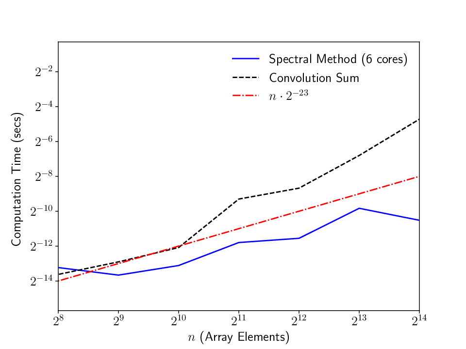
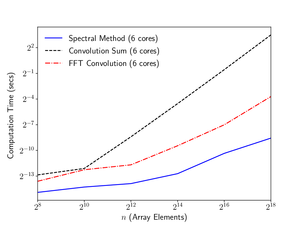
We note that, in 1D, the computation time of using a direct convolution sum (parallelized) to compute the integral term of the original system (10) has complexity $O(N_{s}^{2})$ (where $N_{s}$ is the number of cells), since a sum is required for each point on the line where the convolution is to be approximated. In contrast, the FFT-based elliptic solver has complexity $O(N_{s}\log(N_{s})+N_{s})$ , where the added $N_{s}$ corresponds to multiplication of coefficients. The difference becomes even more significant in higher dimensions, as explained in Section IV. Fig. 2 presents a quantitative comparison.

IV Higher Dimensions

The methodology outlined above is scalable and can be generalized to higher dimensions, as shown next.

IV-A Screened Poisson Mediated Flocking in Radially Symmetric Domain

It seems natural for the interaction function $\psi$ to be radially symmetric, which suggests that the domain $D$ has radial symmetry as well. In higher dimensions, i.e. for $d=2,3$ , this results in singular kernels $\psi$ [30]. Singular kernels have been extensively studied in the literature and, under mild assumptions in the initial conditions, have been shown to result in flocking behavior while, at the same time, avoiding collisions [30]. In this case, we have the BVP of the augmented system of PDEs (14) defined in the radially symmetric domain $D:=\left\{x\in\mathbb{R}^{d}:\|x\|<L/2\right\}$ , with the linear differential operator $\mathcal{L}_{x}$ defined as

\mathcal{L}_{x}=-k^{-d/2}(\nabla_{x}^{2}-\lambda^{2})

(41)

It can be shown ([14]) that this operator is associated with a Green’s function of the form

\displaystyle\psi(x,s)=\bar{\psi}(x-s)+\phi(x,s)

(42)

where $\bar{\psi}$ is given by

	$\displaystyle\bar{\psi}(x,s)$	$\displaystyle=\tilde{\psi}(\\|x-s\\|)$		(43)
		$\displaystyle=\left(\frac{k}{2\pi}\right)^{d/2}\left(\frac{\lambda}{\\|x-s\\|}\right)^{d/2-1}K_{d/2-1}(\lambda\\|x-s\\|)$		(43)

with $K_{\alpha}(\cdot)$ being the modified Bessel function of the second kind of order $\alpha$ , and

\phi(x,s)=-\tilde{\psi}(\frac{2}{L}\|x\|\|s-\frac{L^{2}}{4}\frac{x}{\|x\|^{2}}\|).

(44)

IV-B Screened Poisson Mediated Flocking in Rectangular Domain

The introduction of the operator $\mathcal{L}_{x}$ allows for the fast computation of the solution of (10) by numerically solving (14). The hyperbolic and elliptic solvers introduced in III-C, however, are computationally costly when not working in a rectangular domain $D$ . For this reason, we define the BVP of the augmented system of PDEs (14) with the same linear differential operator $\mathcal{L}_{x}$ defined as

\mathcal{L}_{x}=-\frac{1}{2k}(\nabla_{x}^{2}-\lambda^{2}),~k>0,\ ,\lambda\in\mathbb{R}

(45)

in a $d$ -dimensional rectangular domain $D:=\left[-\nicefrac{{L}}{{2}},\nicefrac{{L}}{{2}}\right]^{d}$ , $L>0$ , with homogeneous Dirichlet boundary conditions. The intuition behind this selection is that $L$ can be chosen large enough to approximately negate the effect of the rectangular domain $D$ on the interaction function $\psi$ as shown in Fig. 4.

Notice that, as shown in Section III-B, $\mathcal{L}_{x}$ is an elliptic, self-adjoint (symmetric) partial differential operator that conserves mass and momentum. Therefore, in two-dimensions, the augmented system (14) takes the form:

\begin{cases}\partial_{t}Q+\partial_{x}F(Q)+\partial_{y}G(Q)=S(Q,\Phi)\\ \mathcal{L}_{x}\Phi=Q\end{cases}

(46)

where $Q:=(\rho,m_{1},m_{2})^{T}$ , $F:=u_{1}Q$ , $G:=u_{2}Q$ , and $S:=(0,\rho\mathcal{L}_{\psi}m-m\mathcal{L}_{\psi}\rho)$ . System (46) can be generalized to three dimensions in the obvious way.

In Fig. 3, we illustrate the density and momentum density field of the solution of system (46) for the initial conditions given in Section VI-B.

In physics and computer graphics, this operator with $\lambda\neq 0$ is associated to the time-independent Klein-Gordon equation and the screened Poisson equation [31]. In the square region $D:=(-\frac{L}{2},\frac{L}{2})\times(-\frac{L}{2},\frac{L}{2})$ with homogeneous Dirichlet boundary conditions, the Green’s function for $\mathcal{L}_{x}$ is given by the solution to

\begin{cases}\mathcal{L}_{x}\psi(x,s)=\delta(x-s)&\text{ for }(x,s)\in D\times D\\ \psi(x,s)=0&\text{ for }(x,s)\in\partial D\times\partial D\end{cases}

(47)

which is the Fourier sine series

	$\displaystyle\psi(x,s)$	$\displaystyle=8k\sum_{m=1}^{\infty}\sum_{n=1}^{\infty}\frac{1}{\mu_{nm}+\lambda^{2}}$		(48)
		$\displaystyle\sin\frac{n\pi}{L}x_{1}^{\prime}\sin\frac{n\pi}{L}s_{1}^{\prime}\sin\frac{m\pi}{L}x_{2}^{\prime}\sin\frac{m\pi}{L}s_{2}^{\prime}$		(48)

where $\mu_{n,m}=(\frac{n\pi}{L})^{2}+(\frac{m\pi}{L})^{2}$ , and $s_{i}^{\prime}=s_{i}+\frac{L}{2}$ , and similarly for $x^{\prime}$ i.e. a translation of coordinates. This may be easily verified by separation of variables, or simply computing $\mathcal{L}_{x}\psi$ . It is obvious $\psi(x,s)$ is symmetric in its arguments, and that it is singular along $x=s$ . Moreover, via Hopf’s maximum principle [27, 32], it is clear immediately that $\psi(x,s)>0$ $\forall(x,s)\in D\times D$ . So, following results in [13, 30], $\psi(x,s)$ can be shown to induce flocking dynamics, as well as collision avoidance.

Numerical approximations to the Green’s function $\psi$ computed via a spectral method are presented here. The behavior of this Green’s function is similar to the 1D Green’s function in $k,\lambda$ , although in the 1D case, the Green’s function has a simple closed-form, and is nonsingular. In Fig. 4, we illustrate the effect of the parameters $k$ , $\lambda$ on the profile of the 2D interaction function. The parameter $k$ has an obvious effect on scaling, and $\lambda$ has the effect of increasing its growth rate. There are singularities along $x=s$ .

IV-C Computational Methods

IV-C1 Hyperbolic Solver

As in the 1D case, we apply the finite volume method [28] to convert the hyperbolic PDE system (14) into a system of ODEs on cells $I_{ij}$ centered on sequence of points $\{(x_{i},y_{j})\}_{i=1,j=1}^{N_{s},N_{s}}$ evenly spaced with spacing $\Delta x=\Delta y$ :

	$\displaystyle\frac{d}{dt}\bar{Q}_{i,j}$	$\displaystyle=-\frac{1}{\Delta x}(F_{i+\frac{1}{2},j}-F_{i-\frac{1}{2},j})$		(49)
		$\displaystyle-\frac{1}{\Delta y}(G_{i,j+\frac{1}{2}}-G_{i,j-\frac{1}{2}})+\bar{S}_{i,j}$		(49)

The interpolated fluxes are given by the Kurganov-Tadmor fluxes analogously to the 1D case ([29]). We use the same time integration and limiting procedure as we do in 1D. The form of the TVD limiter of the Kurganov-Tadmor flux changes slightly in 2D. See [29] for details.

IV-C2 Elliptic Solver

To solve the elliptic equations, we employ spectral methods, as in 1D. A basis for $L^{2}((0,L)^{2};\mathbb{R})$ with zero BCs is

\left\{b_{n,m}(x,s):=\sin\frac{n\pi x}{L}\sin\frac{m\pi s}{L}\right\}_{n=1,m=1}^{\infty,\infty}

(50)

As in the 1D case, candidate solutions to the elliptic BVP for fixed $t$ are Fourier sine series:

\phi(x,s,t)=\sum_{n,m=1}^{\infty}\hat{\phi}_{n,m}(t)b_{n,m}(x^{\prime},s^{\prime}),

(51)

where $s^{\prime}=s+\frac{L}{2}$ and similarly for $x^{\prime}$ . Now, we apply the 2D operator $\mathcal{L}_{x}$ to $\phi$ , which yields:

\sum_{n,m=1}^{\infty}\frac{1}{2k}(\mu_{n,m}+\lambda^{2})\hat{\phi}_{n,m}(t)b_{n,m}(x^{\prime},s^{\prime})=q(x^{\prime},s^{\prime},t)

(52)

Now, let $\hat{q}_{n,m}(t)$ denote the $n,m-$ th Fourier sine coefficient for $q(x^{\prime},s^{\prime},t)$ . Considering an approximation to $\phi$ with $N_{s}^{2}$ harmonics ( $N_{s}$ in each direction) corresponding to the same $N_{s}$ as in the hyperbolic solver, we obtain the semi-discrete spectral method:

\hat{\phi}_{n,m}(t)=\frac{2k\hat{q}_{n,m}(t)}{\mu_{n,m}+\lambda^{2}},\text{ }1\leq n\leq N_{s},1\leq m\leq N_{s}

(53)

where $\mu_{n,m}:=(\frac{n\pi}{L})^{2}+(\frac{m\pi}{L})^{2}$ are the eigenvalues of the Laplacian with Dirichlet BCs. We apply the multidimensional extension of the transforms used in the 1D case to implement this spectral method.

Remark 3.

We note that, compared to Remark 2, in higher dimensions, i.e., 2D and 3D, one can take advantage of the divide-and-conquer approach of FFTs as well as parallelization. While a direct 2D convolution sum has complexity $O(N_{s}^{4})$ , since one needs to compute a double-sum for each grid point desired, the FFT-based elliptic solver has complexity $O(2N_{s}^{2}\log(N_{s})+N_{s}^{2})$ . Please refer to Fig. 2 for quantitative results.

V Learning the Coordination Laws

We utilize the methodology and the computational methods described above to efficiently compute the macroscopic quantities, i.e. the momentum and density of the swarm, as a solution to the augmented system of equations (14). We now incorporate the computation of the swarm’s momentum and density in an iterative learning scheme to estimate the parameters of the interaction function $\psi$ .

We formulate the process of learning the interaction function $\psi$ from density data as a PDE-constrained optimization problem:

\min_{k,\lambda}\sum_{\tau=t_{0}}^{t_{f}}D_{KL}(P^{*}(\tau)||P(\tau))

(54)

where $P^{*}(t)$ and $P(t)$ are probability measures that have densities $\rho^{*}(t,\cdot)$ and $\rho(t,\cdot)$ , the observed and simulated mean-field densities, respectively. The density $\rho^{*}$ is assumed given by observation. The mean-field density $\rho$ associated with $P$ , is subject to the system of PDEs (14) and therefore dependent on the parameter vector $\theta:=(k,\lambda)$ . The Kullback-Leibler (KL) divergence $D_{KL}$ in (54) is given by:

D_{KL}(P_{i}||P_{j}):=\int_{\Omega}\log_{2}\frac{dP_{i}}{dP_{j}}dP_{i}=\int_{D}\rho_{i}\log_{2}\frac{\rho_{i}}{\rho_{j}}dx

(55)

The values of $\rho(t,\cdot),\rho^{*}(t,\cdot)$ are evaluated at the sequence of points $x_{k}$ generated by the finite volume method as described above, i.e. an approximation (more precisely, a piecewise-constant discretization) of the densities is needed, which is either observed or computed by trajectory observations (see Section VI). We approximate the solution $\theta^{*}$ of (54) with respect to $V_{d}(\theta):=\sum_{\tau=t_{0}}^{t_{f}}D_{KL}(P^{*}(\tau)||P(\tau))$ , with the iterative scheme

\theta^{n+1}=-\hat{\mathbf{H}}^{-1}(\theta^{n})\nabla_{\theta}V_{d}(\theta^{n})

(56)

where $\hat{\mathbf{H}}$ is a positive-definite approximation of the Hessian computed via the Lanczos iteration [33]. The gradient is computed by the usual two-point finite difference formula. The KL divergence is approximated by a Riemann sum over the support of the observed density which is sampled over the same grid of points as the approximated density.

We note that in each iteration of the learning algorithm, the solution of the BVP associated with the system of PDEs (10) must be numerically computed, which has become feasible due to the computational advantages originating from the use of the proposed linear operator $\mathcal{L}_{x}$ in (15) (see Remarks 2, 3).

V-A Learning the Interaction Function from Particle Trajectories

In order to better understand the computational advantages of the proposed methodology, we compare it here with a standard learning approach using trajectory data of the position and velocity $\left\{(x_{i},v_{i})\right\}_{i=1}^{N}$ of each particle for some large but finite number of particles $N$ . In general, this problem is a nonlinear system identification problem with known system form given by (1) and unknown interaction function ${\psi:\mathbb{R}^{d}\times\mathbb{R}^{d}\rightarrow\mathbb{R}}$ .

Because of the nonlinearity of (1) and the dependence of the right hand side on every pair $\left((v_{i},v_{j})\right)$ and $\left((x_{i},x_{j})\right)$ , $i\neq j$ , system identification requires the solution of an ODE-constrained optimization problem of dimension $O(N^{2})$ , which has a complexity of $O(N^{2}N_{s}^{2})$ . As a result, it is apparent that for large number of particles $N\gg N_{s}$ , the proposed mean-field methodology is quite faster (see Remarks 2, 3).

An energy-based approach is given in [7], where it is shown that the Cucker-Smale model (1) is equivalent to a fully connected N-dimensional network of generalized mass-spring-dampers with appropriately defined Hamiltonian functions, that can be written in an input-state-output port-Hamiltonian form [19]:

\dot{z}=[J(z)-R(z)]\frac{\partial H(z)}{\partial z}

(57)

where $z=(q,p)$ , with $q,p\in\mathbb{R}^{\frac{N(N-1)}{2}}$ being the vectors of relative distances and momenta between each pair of particles, and the quantities $J=-J^{T}$ , $H$ and $R$ are appropriately defined. The dependence of (57) on the interaction function $\psi$ is introduced by the resistive term $R=R(\psi)$ [7], and is modeled as an artificial neural network with a single hidden layer. The parameters are represented by a vector $\theta$ and the learning process is formulated as a least-squares optimization problem

\min_{\theta}\sum_{\tau=t_{0}}^{t_{f}}\|\dot{z}^{*}(\tau)-\dot{z}(\tau)\|^{2}

(58)

where $z^{*}$ represent the observed trajectories, and $z$ are subject to (57), and the solution $\theta^{*}$ of (58) with respect to $V_{p}(\theta):=\sum_{\tau=t_{0}}^{t_{f}}\|\dot{z}^{*}(\tau)-\dot{z}(\tau)\|^{2}$ , is approached by an iterative gradient descent method

\theta^{n+1}=\theta^{n}-\alpha_{n}(\nabla_{\theta}V_{p}(\theta^{n})),~n=0,1,2,\ldots

(59)

where the iteration maps $\alpha_{n}:\mathbb{R}^{2}\rightarrow\mathbb{R}^{2}$ , ${n\geq 0}$ are defined in accordance with the Adam method of moments for stochastic optimization [34], and the computation of the gradient vectors is implemented using automatic differentiation [35]. It is clear that the dimension of the dynamical system to be solved within the optimization problem grows quadratically with the number of particles $N$ , affecting the scalability of such approaches. Moreover, the quality of the observed trajectory data is crucial for the performance of the learning algorithm.

We note, however, that there is a potential advantage in using the proposed interaction function model (17), (18), even in learning the interaction dynamics of a swarm from particle trajectories. First, the number of parameters to be estimated is greatly reduced, compared to a general regression function such as a neural network [7], or a mixture of Gaussians [11], which reduces the amount of data required for convergence. Secondly, every update in the optimization algorithm improves the estimate of the interaction function over the entire domain $D$ , and not only over a small subset $D_{o}\subset D$ where the distances between each pair of interacting particles happen to be observed. This can result in faster, and, more importantly, robust estimation of the interaction function.

Finally, as an alternative to solving (58), in case observations of the particle trajectories are available, we can always numerically integrate to approximate $\rho$ and use this approximation in our density-based learning algorithm. We will follow this approach when comparing the experimental results in the one-dimensional case in Section VI.

VI Numerical Results

VI-A One-dimensional Case

We illustrate our results in the domain $D=[-\pi,\pi]$ ( $L=2\pi$ ), with initial density and bulk velocity given by

	$\displaystyle\rho_{0}(\hat{x})$	$\displaystyle=\frac{\pi}{2L}\cos\frac{\pi\hat{x}}{L},$		(60)
	$\displaystyle u_{0}(\hat{x})$	$\displaystyle=-\sin\frac{\pi\hat{x}}{L},\ \hat{x}\in D,\ c>0$		(61)

i.e. assuming that $\rho_{0}(\hat{x})=u_{0}(\hat{x})=0,\ \forall\hat{x}\notin D$ , where $\hat{x}$ is as defined in (5). In order to accurately evaluate the learning scheme defined in Section V, we obtain the empirical density evolution data $\rho*$ by first simulating the particle equations (1) with initial conditions randomly generated from the initial density and bulk velocity (61), and then taking the piecewise-constant density discretization

\rho^{*}[t_{i},x_{s}]:=\frac{1}{N_{s}\lambda(I_{j})}\mu(\{x_{k}([t_{i}]\in I_{j}\})

(62)

where $\lambda(\cdot)$ is the Lebesgue measure, $\mu(\cdot)$ is the counting measure, and $I_{i}$ , $x_{j}$ are defined as in the formulation of the finite volume method (Section III-C). To showcase the robustness of our approach to noisy observations, we add a Gaussian noise $\epsilon_{n}\sim N(0,\sigma_{n}^{2})$ with $\sigma_{n}^{2}=1$ to the trajectory data. We choose an interaction function $\psi^{*}$ of the form (17), (18) with $(\hat{k}^{*},\hat{\lambda}^{*})=(4,1)$ . The system of particle equations is numerically solved using the velocity Verlet algorithm [11], which, given a system of ODEs of the form

\begin{cases}\frac{dx}{dt}&=v\\ \frac{dv}{dt}&=a(x,v,t),\end{cases}

(63)

with appropriate initial conditions and a time-discretization at steps $\{0,1,...,i,...\}$ with increment $\Delta t$ , takes the form

\begin{split}v_{i+\frac{1}{2}}&=v_{i}+\frac{1}{2}a(x_{i},v_{i},t_{i})\Delta t\\ x_{i+1}&=x_{i}+\Delta tv_{i+\frac{1}{2}}\\ v_{i+1}&=v_{i}+\frac{\Delta t}{2}[a(x_{i},v_{i},t_{i})+a(x_{i+1},v_{i+\frac{1}{2}},t_{i+1})].\end{split}

(64)

The agreement between the solutions of the particle model (1) and the macro-scale model (14) for $N_{s}=2\cdot 10^{4}$ , $\Delta t=.01$ , and cell $\Delta x=\frac{2\pi}{101}$ , and is shown in Fig. 5. The training error and the reconstructed interaction function are depicted in Fig. 6. The parameters $(\hat{k}^{*},\hat{\lambda}^{*})=(3.98721701,0.98546559)\sim(4,1)$ of the interaction function $\psi$ were recovered and the Newton’s iteration converged in 11 iterations.

As a second experiment, in order to illustrate the expressiveness of the proposed family of interaction functions (17), (18), and assess the generalizability of the proposed methodology, we obtain the “observed” density evolution by simulating system (1) with the original Cucker-Smale interaction function

\psi_{CS}(x,y)=\psi^{*}(x-y)=\frac{K^{*}}{(1+\|x-y\|^{2})^{\gamma^{*}}}

(65)

for $(K^{*},\gamma^{*})=(5,2)$ .

The training error and the reconstructed interaction function are depicted in Fig. 7. We observe that the reconstruction is not ideal but closely resembles the original interaction function, while the reconstruction error of the density evolution of the swarm is negligible. These results validate our hypothesis that the proposed interaction functions can model a wide range of collective behaviors, mostly because the model parameters can control the pairwise communication of the swarm’s agents without affecting the flocking behavior.

We note that problem (54) is generally a non-convex optimization problem, and may be sensitive to initial estimates of the parameters $(k,\lambda)$ leading to sub-optimal solutions $(\hat{k}^{*},\hat{\lambda}^{*})\neq(k^{*},\lambda^{*})$ . In addition, the discretized objective function for the densities $V_{d}$ may approach very small values although $(\hat{k}^{*},\hat{\lambda}^{*})\neq(k^{*},\lambda^{*})$ , suggesting that, for a given set of observation data, certain non-global minima of (54) can produce an accepted solution for the underlying interaction function of the swarm. In this case, the reconstructed parameters $(\hat{k}^{*},\hat{\lambda}^{*})$ can be used to accurately reconstruct the actual observed trajectories.

VI-B Two-dimensional Case

We illustrate our results in the domain $D=[-\pi,\pi]\times[-\pi,\pi]$ , i.e. for $L=2\pi$ , with initial density and bulk velocity given by

	$\displaystyle\rho_{0}(\hat{x},\hat{y})$	$\displaystyle=\frac{\pi^{2}}{4L^{2}}\cos\frac{\pi\hat{x}}{L}\cos\frac{\pi\hat{y}}{L},$		(66)
	$\displaystyle u_{0}(\hat{x},\hat{y})$	$\displaystyle=-\frac{1}{4}(\sin\frac{\pi\hat{x}}{L},\sin\frac{\pi\hat{y}}{L})^{T},\hat{x},\hat{y}\in[-\pi,\pi]$		(67)

i.e. assuming that $\rho_{0}(\hat{x})=u_{0}(\hat{x})=0,\ \forall\hat{x}\notin D$ . We note that these initial conditions and compact domain, again refer to the fluctuation variables $\hat{x}$ defined in (5).

In the two-dimensional case, we obtain the density data observations by directly solving the mean-field equations (10) for two different Cucker-Smale models. First we solve (46) with the operator $\mathcal{L}_{x}$ as defined in (15) for $(\hat{k}^{*},\hat{\lambda}^{*})=(4,1)$ . An illustration of the density $\rho^{*}$ and momentum $m^{*}$ evolution over time is given in Fig. 3. The training error for our learning scheme is depicted in Fig. 8. The parameters $k,\lambda$ were estimated as $(\hat{k}^{*},\hat{\lambda}^{*})=(4.01514,1.00194)$ .

Similar to the one-dimensional case, we test the generalizability of the proposed methodology, by obtaining the density evolution observations by directly solving the Eulerian equations (10) with the original Cucker-Smale interaction function $\psi^{*}$ in (65) for $(K^{*},\gamma^{*})=(5,2)$ .

For the integral parts of (10) of the form

\phi(x,t)=\int_{D}\psi^{*}(x-s)q(s,t)ds=\int_{\mathbb{R}^{2}}\psi^{*}(x-s)q(s,t)ds,

(68)

where $\psi^{*}$ are square-integrable kernels and $q$ compactly supported on square region $D$ , we employ Fourier transform-based convolution. Via the properties of the convolution [27], and denoting $\hat{\phi}(\xi,t),\hat{\psi}(\xi),\hat{q}(\xi,t)$ as the Fourier coefficients of the given functions, we apply the Fourier transform in $\mathbb{R}^{2}$ , which gives:

\hat{\phi}(\xi,t)=\hat{\psi}(\xi)\hat{q}(\xi,t).

(69)

To implement this formula, we use the usual $2N_{s}$ zero-padded FFT on the regularly spaced points given in the hyperbolic solver to compute the coefficients and approximate the convolution integrals. This prevents circular convolution.

The training error is depicted in Fig. 8. Similar to the results in Fig. 7,we expect that the reconstruction of the interaction function may not be ideal but can closely approximate the original interaction function, while the reconstruction error of the density evolution of the swarm gets minimized. These results validate our hypothesis that the proposed interaction functions can model a wide range of collective behaviors in multi-dimensional space.

VII Conclusion and Discussion

We have considered the problem of understanding the coordinated movements of biological or artificial swarms. While current learning methodologies mainly use agent-based models, accurate observations of the position and velocity trajectories of each agent are required. Because of the difficulty to extract such observations in real life, we have proposed a learning scheme to reconstruct the coordination laws of the interacting agents from observations of the swarm’s density evolution over time. We believe that developing learning algorithms based on the macroscopic quantities of the swarm can play an important role in the analysis of collective motion and has mainly been inhibited due to the computational expense of solving the corresponding mean-field hydrodynamic equations. The results of this work can be used to model and understand biological and artificial flocks, and design controllers for large networked systems and robotic swarms. Moreover, the identification of the coordination laws of an observed swarm through its density evolution over time, can lead to the development of fast defensive mechanisms against adversarial swarm attacks.

References

[1] A. Okubo, “Dynamical aspects of animal grouping: swarms, schools, flocks, and herds,” Advances in biophysics, vol. 22, pp. 1–94, 1986.
[2] C. Reynolds, “Flocks, herds and schools: A distributed behavioral model,” in ACM SIGGRAPH computer graphics, vol. 21, no. 4. ACM, 1987, pp. 25–34.
[3] F. Cucker and S. Smale, “Emergent behavior in flocks,” IEEE Transactions on automatic control, vol. 52, no. 5, pp. 852–862, 2007.
[4] I. Giardina, “Collective behavior in animal groups: theoretical models and empirical studies,” HFSP journal, vol. 2, no. 4, pp. 205–219, 2008.
[5] M. Ballerini, N. Cabibbo, R. Candelier, A. Cavagna, E. Cisbani, I. Giardina, V. Lecomte, A. Orlandi, G. Parisi, A. Procaccini et al., “Interaction ruling animal collective behavior depends on topological rather than metric distance: Evidence from a field study,” Proceedings of the national academy of sciences, vol. 105, no. 4, 2008.
[6] I. L. Bajec and F. H. Heppner, “Organized flight in birds,” Animal Behaviour, vol. 78, no. 4, pp. 777–789, 2009.
[7] I. Matei, C. Mavridis, J. S. Baras, and M. Zhenirovskyy, “Inferring particle interaction physical models and their dynamical properties,” in 2019 IEEE Conference on Decision and Control (CDC). IEEE, 2019, pp. 4615–4621.
[8] C. N. Mavridis, N. Suriyarachchi, and J. S. Baras, “Detection of dynamically changing leaders incomplex swarms from observed dynamic data,” in 2020 Conference on Decision and Game Theory for Security (GameSec), 2020.
[9] M. Nagy, Z. Ákos, D. Biro, and T. Vicsek, “Hierarchical group dynamics in pigeon flocks,” Nature, vol. 464, pp. 890–893, 2010.
[10] F. Lu, M. Zhong, S. Tang, and M. Maggioni, “Nonparametric inference of interaction laws in systems of agents from trajectory data,” arXiv preprint arXiv:1812.06003, 2018.
[11] Z. Mao, Z. Li, and G. E. Karniadakis, “Nonlocal flocking dynamics: Learning the fractional order of pdes from particle simulations,” Communications on Applied Mathematics and Computation, vol. 1, no. 4, pp. 597–619, 2019.
[12] J. A. Carrillo, M. Fornasier, G. Toscani, and F. Vecil, “Particle, kinetic, and hydrodynamic models of swarming,” in Mathematical modeling of collective behavior in socio-economic and life sciences. Springer, 2010, pp. 297–336.
[13] R. Shvydkoy and E. Tadmor, “Eulerian dynamics with a commutator forcing ii: Flocking,” arXiv preprint arXiv:1701.07710, 2017.
[14] C. N. Mavridis, A. Tirumalai, J. S. Baras, and I. Matei, “Semi-linear poisson-mediated flocking in a cucker-smale model,” in 24th International Symposium on Mathematical Theory of Networks and Systems (MTNS), 2021.
[15] C. Sinigaglia, A. Manzoni, and F. Braghin, “Density control of large-scale particles swarm through pde-constrained optimization,” arXiv preprint arXiv:2104.06373, 2021.
[16] K. Elamvazhuthi and S. Berman, “Mean-field models in swarm robotics: a survey,” Bioinspiration & biomimetics, vol. 15, no. 1, p. 015001, 2019.
[17] M. Fornasier and F. Solombrino, “Mean-field optimal control,” ESAIM: Control, Optimisation and Calculus of Variations, vol. 20, no. 4, pp. 1123–1152, 2014.
[18] D. Chen, T. Vicsek, X. Liu, T. Zhou, and H.-T. Zhang, “Switching hierarchical leadership mechanism in homing flight of pigeon flocks,” EPL (Europhysics Letters), vol. 114, no. 6, p. 60008, 2016.
[19] A. van der Schaft and D. Jeltsema, “Port-hamiltonian systems theory: An introductory overview,” Foundations and Trends® in Systems and Control, vol. 1, no. 2-3, pp. 173–378, 2014. [Online]. Available: http://dx.doi.org/10.1561/2600000002
[20] C. N. Mavridis, A. Tirumalai, and J. S. Baras, “Learning interaction dynamics from particle trajectories and density evolution,” in 2020 59th IEEE Conference on Decision and Control (CDC). IEEE, 2020.
[21] S.-Y. Ha, J.-G. Liu et al., “A simple proof of the cucker-smale flocking dynamics and mean-field limit,” Communications in Mathematical Sciences, vol. 7, no. 2, pp. 297–325, 2009.
[22] C. Lancellotti, “On the vlasov limit for systems of nonlinearly coupled oscillators without noise,” Transport theory and statistical physics, vol. 34, no. 7, pp. 523–535, 2005.
[23] F. Golse, “The mean-field limit for the dynamics of large particle systems,” Journées équations aux dérivées partielles, pp. 1–47, 2003.
[24] J. K. Truelove, R. I. Klein, C. F. McKee, J. H. H. II, L. H. Howell, J. A. Greenough, and D. T. Woods, “Self-gravitational hydrodynamics with three-dimensional adaptive mesh refinement: Methodology and applications to molecular cloud collapse and fragmentation,” The Astrophysical Journal, vol. 495, no. 2, pp. 821–852, mar 1998.
[25] R. E. Shiffler and P. D. Harsha, “Upper and lower bounds for the sample standard deviation,” Teaching Statistics, vol. 2, no. 3, pp. 84–86, 1980.
[26] M. Taylor, Partial Differential Equations I: Basic Theory, ser. Applied Mathematical Sciences. Springer New York, 2010.
[27] L. Evans, Partial Differential Equations, ser. Graduate studies in mathematics. American Mathematical Society, 1998. [Online]. Available: https://books.google.com/books?id=5Pv4LVB_m8AC
[28] R. J. LeVeque, Finite Volume Methods for Hyperbolic Problems, ser. Cambridge Texts in Applied Mathematics. Cambridge University Press, 2002.
[29] A. Kurganov and E. Tadmor, “New high-resolution central schemes for nonlinear conservation laws and convection–diffusion equations,” Journal of Computational Physics, vol. 160, no. 1, pp. 241 – 282, 2000.
[30] S. Ahn, H. Choi, S.-Y. Ha, and H. Lee, “On collision-avoiding initial configurations to cucker-smale type flocking models,” Communications in Mathematical Sciences, vol. 10, 06 2012.
[31] P. Bhat, B. Curless, M. Cohen, and L. Zitnick, Fourier Analysis of the 2D Screened Poisson Equation for Gradient Domain Problems, 2008.
[32] K. Kreith, “Criteria for positive green’s functions,” Illinois J. Math., vol. 12, no. 3, pp. 475–478, 09 1968. [Online]. Available: https://doi.org/10.1215/ijm/1256054114
[33] S. G. Nash, “Newton-type minimization via the lanczos method,” SIAM Journal on Numerical Analysis, vol. 21, no. 4, pp. 770–788, 1984. [Online]. Available: https://doi.org/10.1137/0721052
[34] D. P. Kingma and J. Ba, “Adam: A method for stochastic optimization,” arXiv preprint arXiv:1412.6980, 2014.
[35] D. Maclaurin, D. Duvenaud, M. Johnson, and J. Townsend, “Autograd,” https://github.com/HIPS/autograd, 2018.

Appendix A Analytic Computation of the 1D Green’s Function $\psi$

The Green’s function $\psi(x,s)$ of the following BVP:

\begin{cases}-\frac{1}{2k}(y^{\prime\prime}-\lambda^{2}y)=f(x)\\ y(-\frac{L}{2})=y(\frac{L}{2})=0\\ -\frac{L}{2}\leq x\leq\frac{L}{2}\end{cases}

takes the form:

\psi(x,s)=\begin{cases}a(s)e^{-\lambda x}+b(s)e^{\lambda x},~x<s\\ c(s)e^{-\lambda x}+d(s)e^{\lambda x},~x>s\end{cases}

The first condition that $\psi(x,s)$ has to satisfy is $\psi(-\frac{L}{2},s)=0$ , which gives:

b(s)=-a(s)e^{\lambda L}

(70)

The second condition is $\psi(\frac{L}{2},s)=0$ , which gives:

d(s)=-c(s)e^{-\lambda L}

(71)

The third condition comes from the continuity of $\psi(x,s)$ at $x=s$ :

a(s)(e^{-\lambda s}-e^{\lambda L}e^{\lambda s})=c(s)(e^{-\lambda s}-e^{-\lambda L}e^{\lambda s})

(72)

and the fourth is the differentiability condition at $x=s$ :

a(s)(e^{-\lambda s}+e^{\lambda L}e^{\lambda s})=c(s)(e^{-\lambda s}+e^{-\lambda L}e^{\lambda s})-\frac{2k}{\lambda}

(73)

Adding (72) and (73) gives:

c(s)=a(s)+\frac{k}{\lambda}e^{\lambda s}

and, in addition, subtracting (73) from (72) gives:

	$\displaystyle a(s)$	$\displaystyle=K(e^{-\lambda s}-e^{\lambda s}e^{-\lambda L})$
	$\displaystyle c(s)$	$\displaystyle=K(e^{-\lambda s}-e^{\lambda s}e^{\lambda L})$

where

K=-\frac{k}{\lambda}\frac{1}{e^{\lambda L}-e^{-\lambda L}}

Therefore, the Green’s function $\psi(x,s)$ takes the form

\psi(x,s)=\begin{cases}K(e^{-\lambda s}-e^{\lambda s}e^{-\lambda L})(e^{-\lambda x}-e^{\lambda x}e^{\lambda L}),~x<s\\ K(e^{-\lambda s}-e^{\lambda s}e^{\lambda L})(e^{-\lambda x}-e^{\lambda x}e^{-\lambda L}),~x>s\end{cases}

which can be equivalently written (by multiplying by $e^{\lambda\frac{L}{2}}e^{-\lambda\frac{L}{2}}$ ) as

\psi(x,s)=\begin{cases}K\sigma_{m}(s)\sigma_{p}(x),~x<s\\ K\sigma_{p}(s)\sigma_{m}(x),~x>s\end{cases}

where

\displaystyle\sigma_{m}(z)=2\sinh\left(\lambda(z-\frac{L}{2})\right),\ \sigma_{p}(z)=2\sinh\left(\lambda(z+\frac{L}{2})\right)

As a final note, it is clear that $\psi(x,s)$ satisfies the symmetry condition:

\psi(x,s)=\psi(s,x).

$\displaystyle\frac{d\|\hat{v}\|^{2}}{dt}$	$\displaystyle=-\frac{1}{N^{2}}\sum_{1\leq i,j\leq N}\psi(\hat{x}_{j},\hat{x}_{i})\\|\hat{v}_{j}-\hat{v}_{i}\\|^{2}$	(24)
	$\displaystyle\leq-\frac{1}{N^{2}}\psi(-2\hat{x}_{M},\lambda\|\hat{x}\|)\sum_{1\leq i,j\leq N}\\|\hat{v}_{j}-\hat{v}_{i}\\|^{2}$
	$\displaystyle\overset{(*)}{=}-2\psi(-2\hat{x}_{M},\lambda\|\hat{x}\|)\|\hat{v}\|^{2}$

$\displaystyle\frac{d}{dt}V(\|\hat{x}\|,\|\hat{v}\|)$	$\displaystyle=\frac{d\|\hat{v}\|}{dt}+\phi(\|\hat{x}\|)\frac{d\|\hat{x}\|}{dt}$	(27)
	$\displaystyle\leq\phi(\|\hat{x}\|)\left(-\|v\|+\frac{d\|\hat{x}\|}{dt}\right)$
	$\displaystyle\leq 0$

	$\displaystyle\mathcal{L}_{x}z=\rho$
	$\displaystyle\mathcal{L}_{x}y=m$

Learning Swarm Interaction Dynamics from Density Evolution

Abstract

Index Terms:

I Introduction

II Mathematical Models and Notation

II-A The Cucker-Smale Model

Definition 1 (Time-Asymptotic Flocking).

II-B The Mean-Field Limit

III Screened Poisson Mediated Flocking

Remark 1.

III-A Asymptotic Flocking

Theorem 1.

Proof.

III-B Conservation of Mass and Momentum

Lemma 2.

Proof.

Proposition 1.

Proof.

III-C Computational Methods

III-C1 Hyperbolic Solver

III-C2 Elliptic Solver

Remark 2.

IV Higher Dimensions

IV-A Screened Poisson Mediated Flocking in Radially Symmetric Domain

IV-B Screened Poisson Mediated Flocking in Rectangular Domain

IV-C Computational Methods

IV-C1 Hyperbolic Solver

IV-C2 Elliptic Solver

Remark 3.

V Learning the Coordination Laws

V-A Learning the Interaction Function from Particle Trajectories

VI Numerical Results

VI-A One-dimensional Case

VI-B Two-dimensional Case

VII Conclusion and Discussion

References

Appendix A Analytic Computation of the 1D Green’s Function ψ\psi

Appendix A Analytic Computation of the 1D Green’s Function $\psi$