Topological graph states and quantum error correction codes

Pengcheng Liao Affiliation: Institute for Quantum Science and Technology and Department of Physics and Astronomy, University of Calgary, Calgary, Alberta T2N 1N4, Canada Barry C. Sanders Affiliation: Institute for Quantum Science and Technology and Department of Physics and Astronomy, University of Calgary, Calgary, Alberta T2N 1N4, Canada David L. Feder Affiliation: Institute for Quantum Science and Technology and Department of Physics and Astronomy, University of Calgary, Calgary, Alberta T2N 1N4, Canada

Abstract

Deciding if a given family of quantum states is topologically ordered is an important but nontrivial problem in condensed matter physics and quantum information theory. We derive necessary and sufficient conditions for a family of graph states to be in TQO-1, which is a class of quantum error correction code states whose code distance scales macroscopically with the number of physical qubits. Using these criteria, we consider a number of specific graph families, including the star and complete graphs, and the line graphs of complete and completely bipartite graphs, and discuss which are topologically ordered and how to construct the codewords. The formalism is then employed to construct several codes with macroscopic distance, including a three-dimensional topological code generated by local stabilizers that also has a macroscopic number of encoded logical qubits. The results indicate that graph states provide a fruitful approach to the construction and characterization of topological stabilizer quantum error correction codes.

I Introduction

Topologically ordered states have been the focus of much research activity because of their novel features and properties in condensed matter physics Qi and Zhang 2011; Wang and Zhang 2017; Rachel 2018 and their potential use in fault-tolerant quantum information processing Kitaev 2003; Mong et al. 2014; Kraus et al. 2013; Sau et al. 2010; Alicea et al. 2011. The characterization and detection of topological order is a non-trivial task in general because of intrinsically long-range entanglement and the difficulty of distinguishing different topological phases using only local operators Chen et al. 2010. Approaches to the characterization of topological order include the entanglement entropyKitaev and Preskill 2006; Levin and Wen 2006, quantum Fisher information Zhang et al. 2018, quantum circuit complexity for state generation Chen et al. 2010, and irreducible multiple-party correlation Zhou 2008; Liu et al. 2016, among others. These suffer from a number of problems. For example, the determination of topological entanglement entropy relies heavily on the smoothness of the boundary; otherwise, subtle correction terms may be needed Papanikolaou et al. 2007; Williamson et al. 2019. State generation complexity also does not provide sufficient information about the topological order; topologically ordered states cannot be prepared within the quantum cicuit model in constant depth Liao and Feder 2021, and there also exist states that cannot be generated in constant depth but are nevertheless not topologically ordered, such as GHZ states and cube states Aharonov and Touati 2018.

There is an important bilateral relationship between quantum error correction codes (QECCs) Lidar and Brun 2013 and topological order. An $[[n,k,d]]$ QECC, where $n$ is the number of qubits, $k$ is the number of logical (encoded) qubits, and $d$ is the code distance, is defined as a subspace of dimension $2^{k}$ ( $1\leq k\leq n$ ) in Hilbert space $\mathscr{H}_{2}^{\otimes n}$ that is able correct arbitrary independent errors that occur on $t=\lfloor(d-1)/2\rfloor$ qubits. On the one hand, QECCs can be constructed from topologically ordered states, such as the toric code Kitaev 2003, color code Bombin and Martin-Delgado 2006, and surface code Dennis et al. 2002. On the other hand, the formulation of QECCs can itself provide a natural characterization of topologically ordered states: QECC states with ‘macroscopic’ distance Bravyi et al. 2010a, i.e. where the code distance $d$ scales as $d\sim n^{c}$ where $0<c\leq 1$ . The quantum states in the macroscopic-distance QECCs are called TQO-1 states.

Graph theory has been used extensively to construct QECCs Schlingemann and Werner 2001; Tonchev 2002; MacKay et al. 2004; Danielsen 2005; Couvreur et al. 2013; Cafaro et al. 2014, providing a rich toolkit for the exploration of topological codes based on graph states. Furthermore, restrictions on the geometrical locality of stabilizer generators or the dimension of physical qubits pose fundamental limits on the performance of stabilizer QECCs Bravyi et al. 2010b; as there are no such restrictions on the graphs associated with stabilizer codes, one can potentially circumvent these limits and construct better LDPC codes. In recent work Liao and Feder 2021, the toric code stabilizer states were mapped to graph states using local Clifford operations Van den Nest et al. 2004, giving a specific graph configuration corresponding to topologically ordered states and opening a new window into the construction of topological codes. The graph associated with the toric code was found to be composed of only two simple graphs (star and half graphs). This naturally leads to the possibility that particular graphs are most conducive to the construction of topological QECCs, and for the characterization of topological order. In this work, we show how to decide if a given family of graphs corresponds to TQO-1 states.

In addition to providing a characterization of topological order, our graph-theoretical framework can be used to construct QECCs with macroscopic distance and macroscopic scaling in the number of encoded qubits. This behavior is expected to be important for fault tolerant logical operations on practical quantum devices, and might also shed light on an quantum complexity. For example, the existence of good quantum low-density parity check (LDPC) codes Kovalev and Pryadko 2013; Breuckmann and Eberhardt 2021, where both $d$ and $k$ scale linearly with $n$ and the weight of the stabilizer generators is constant, is related to important quantum complexity problems Aharonov et al. 2013; Eldar and Harrow 2017; Freedman and Hastings 2013, so the exploration of topological codes might shed light on this open quantum complexity problem. Most generally, the construction of new topological codes provides insights about the nature of the special order underpinning topological states.

In this work, we derive necessary and sufficient conditions for graph states to be topologically ordered, under the definition of TQO-1. To illustrate the use of this condition, we first discuss several families of graph states that are not in TQO-1: graphs with constant vertex degree, and the star and complete graphs whose maximum vertex degree grows with the number of vertices. We then show that, in contrast, the family of graph states corresponding to multiple copies of the star graph is in TQO-1, as are the graphs associated with the toric code (hitherto referred to as the toric graph), and the line graphs of the complete graph and the complete bipartite graph; the last three all correspond to $[[n,1,\sqrt{n}]]$ QECCs. By embedding a classical LDPC code into the multi-star graph state, we can also obtain a $[[ckd,k,d]]$ QECC where $c$ is an independent constant. These families of states all share a common feature, which is necessary (but not sufficient) for the graphs to be in TQO-1: the maximum vertex degree must scale macroscopically. Using these insights, we construct a topological QECC based on a generalization of the toric graph. This QECC corresponds to qubits located on the vertices of a three-torus, stabilized by six-local Pauli operators, and corresponds to a $[[n,n^{1/3},n^{1/3}]]$ QECC. The distance and the number of logical qubits of our constructed code is similar to some of the known 3D topological codes Vijay et al. 2016; Bravyi et al. 2011; Shirley et al. 2019.

This work is organized as follows. The background information is reviewed in Sec. II. The criteria for a family of graph states to be in TQO-1 are derived in Sec. III. In Sec. IV, several families of graph states are discussed that both do and do not satisfy the criteria for TQO-1. For these graph state that are TQO-1, QECCs with macroscopic distance are also constructed from the graph states. Sec. V provides an example of a topological QECC derived from an extension of the toric graph, with qubits on the vertices of three-torus. The results are discussed in Sec. VI. Some technical details are included in the appendices.

II Background

In this section, the background formalism to the main results is provided. Key definitions and concepts include the TQO-1 class, the quantum error correction conditions, graph theory, and graph states. Some of the definitions are rephrased so that they can be repurposed for this work.

II.1 TQO-1 class and QECC condition

This subsection provides a review of the class of quantum states called TQO-1 Bravyi et al. 2010a. This class is defined using QECC and captures some of the main features of topological order. As TQO-1 is described using QECC, the quantum error correction conditions are also discussed.

The state $\Ket{\mathbf{x}}$ is the computational basis state labeled by $\mathbf{x}\in\set{0,1}^{n}$ in the $n$ -qubit Hilbert space $\mathscr{H}_{2}^{\otimes n}$ . A quantum state is understood to mean a trace-class positive-definite operator on Hilbert space, and a pure state is any idempotent operator in this class. Each pure state is identified with a specific vector in the Hilbert space. We define $\mathbf{P}_{*}(\mathbb{C}):=\bigoplus_{n\in\mathbb{N}}\mathbf{P}_{2^{n}}(\mathbb{C})$ , the direct sum of all complex projective spaces of dimension that is a power of 2; here, $\mathbb{N}_{s}\subseteq\mathbb{N}$ is a subset of integers containing countably infinite elements.

Definition 1 (Quantum-state oracle).

A quantum-state oracle

\textsc{qState}:\mathbb{N}_{s}\to\mathbf{P}_{*}(\mathbb{C}):n\mapsto\psi_{n}:=\begin{pmatrix}\alpha_{0}\\ \vdots\\ \alpha_{2^{n}-1}\end{pmatrix}

(1)

maps a non-negative integer to a vector in a complex projective space.

Definition 2 (Family of quantum states).

Given qState, a family of quantum states for this oracle is $\mathtt{S}:=\Set{\Ket{\psi_{n}}\in\mathscr{H}_{2}^{\otimes n}}_{n\in\mathbb{N}_{s}}$ , where

\Ket{\psi_{n}}:=\sum_{\mathbf{x}\in\set{0,1}^{n}}\alpha_{\mathbf{x}}\Ket{\mathbf{x}}.

(2)

Whenever the term ‘a family of quantum states’ is used in this work, a qState oracle and $\mathbb{N}_{s}$ are implied and are often not stated explicitly. For $N\in\mathbb{N}$ , $\left(\mathbf{P}_{N}(\mathbb{C})\right)^{\otimes*}:=\bigoplus_{i\in[N]}\left(\mathbf{P}_{N}(\mathbb{C})\right)^{\otimes i}$ is the direct of sum of $i$ -fold ( $i\in[N]:=\set{1,\ldots,N}$ ) $N$ -dimensional complex projective spaces, and $\left(\mathbf{P}_{*}(\mathbb{C})\right)^{\otimes*}:=\bigoplus_{n}\left(\mathbf{P}_{2^{n}}(\mathbb{C})\right)^{\otimes*}$ .

Definition 3.

A quantum-code oracle maps two non-negative integers $n$ and $k$ to $2^{k}$ independent vectors in the complex projective space $\mathbf{P}_{2^{n}}(\mathbb{C})$ :

	qCode	$\displaystyle:\mathbb{N}\times\mathbb{N}\to\left(\mathbf{P}_{}(\mathbb{C})\right)^{\otimes}$		(3)
		$\displaystyle:(n,k)\mapsto(\psi_{n}^{(0)},\ldots,\psi_{n}^{(2^{k}-1)}).$

Definition 4 (Family of subspaces).

Given a qCode oracle and function $k:\mathbb{N\to\mathbb{N}}$ , a family of subspaces is

\mathtt{C}=\Set{\mathscr{C}_{n}:=\operatorname{span}\Set{\Ket{\psi_{n}^{(0)}},\ldots,\Ket{\psi_{n}^{(2^{k_{n}}-1)}}}}_{n\in\mathbb{N}_{s}},

(4)

where $\psi_{n}^{(i)}$ is one of the vectors in the range of $\textsc{qcode}(n,k_{n})$ and $\Ket{\psi_{n}^{(i)}}\in\mathscr{H}_{2}^{\otimes n}(0\leq i\leq 2^{k_{n}}-1)$ is constructed according to Eq. (2).

Definition 5 (Family of QECCs).

Given a family of subspaces $\mathtt{C}=\Set{\mathscr{C}_{n}}_{n\in\mathbb{N}_{s}}$ and $d:\mathbb{N}\to\mathbb{N}$ , if every $\mathscr{C}_{n}\in\mathtt{C}$ is also a QECC of distance $d_{n}$ , then $\mathtt{C}$ is a family of $[[n,k,d]]$ QECCs.

In this work, whenever the ‘family of subspaces / codes’ term is employed, functions $k$ and $d$ are implied yet not always stated explicitly. A family of $[[n,k,d]]$ QECCs has ‘macroscopic distance’ if $d\in\operatorname{sublin}(n):=\cup_{0<c\leq 1}\Theta(n^{c})$ , which is the set of polynomials with power less than 1.

Definition 6 (Class TQO-1).

TQO-1 is the set of families of quantum states such that for every family $\mathtt{S}=\Set{\Ket{\psi_{n}}}_{n\in\mathbb{N}_{s}}\in\text{TQO-1}$ , there exists a family of macroscopic-distance QECCs $\mathtt{C}=\Set{\mathscr{C}_{n}}_{n\in\mathbb{N}_{s}}$ , satisfying $\Ket{\psi_{n}}\in\mathscr{C}_{n}\forall n\in\mathbb{N}_{s}$ .

In order to evaluate the distance of a QECC, we restate the quantum error correction condition from Knill and Laflamme 1997; Nielsen and Chuang 2000. Let $\mathcal{D}(\mathscr{H}_{2}^{\otimes n})$ denote the set of density matrices on $n$ qubits.

Theorem 1 (Quantum error correction condition Knill and Laflamme 1997; Nielsen and Chuang 2000).

Suppose $\mathscr{C}\subset\mathscr{H}_{2}^{\otimes n}$ is a QECC, $P$ is the projector into $\mathscr{C}$ from $\mathscr{H}_{2}^{\otimes n}$ , $\mathcal{E}:\mathcal{D}(\mathscr{H}_{2}^{\otimes n})\to\mathcal{D}(\mathscr{H}_{2}^{\otimes n})$ is a quantum channel with Kraus operators $\left\{E_{i}\right\}_{i\in[2^{n}]}$ . A necessary and sufficient condition for the existence of an error-correction operation $\mathcal{R}$ correcting $\mathcal{E}$ on $\mathscr{C}$ is that

PE_{i}^{\dagger}E_{j}P=\alpha_{ij}P

(5)

for some Hermitian matrix $\alpha\in\mathbb{C}^{2^{n}\times 2^{n}}$ .

A simplified quantum error correction condition derived from the Theorem 1 is used later in this work. The Pauli group on $n$ qubits is $\mathcal{P}_{n}:=\set{\pm i,\pm 1}\times\set{I,X,Y,Z}^{\otimes n}$ , where $X,Y,Z$ are 1-qubit Pauli operators. The weight of a Pauli operator $\text{wt}(O)$ corresponds to the number of qubits acted on by $O$ non-trivially. Then, $\mathcal{P}_{n}^{t}:=\{O\in\mathcal{P}_{n}|w(O)\leq t\}$ contains every operator in the Pauli group whose weight is no greater than $t$ .

Corollary 1.

Given $d<n\in\mathbb{N}$ and two states $\Ket{\phi},\Ket{\psi}\in\mathscr{H}_{2}^{\otimes n}$ , then $\operatorname{span}_{\mathbb{C}}\{\Ket{\phi},\Ket{\psi}\}\subseteq\mathscr{H}_{2}^{\otimes n}$ is a $[[n,1,d]]$ QECC iff

	$\displaystyle\braket{\phi\|O\|\phi}=$	$\displaystyle\braket{\psi\|O\|\psi}$		(6)
	$\displaystyle\braket{\phi\|O\|\psi}=$	$\displaystyle 0$		(7)

hold $\forall O\in\mathcal{P}_{n}^{d-1}$ .

Proof.

A quantum error code of distance $d$ can correct any errors on less than or equal to $t=\frac{d-1}{2}$ qubits. Thus, to prove $C$ is a distance- $d$ code is equivalent to proving that $\mathcal{P}_{n}^{t}$ is a set of correctable errors on $C=\operatorname{span}_{\mathbb{C}}\{|\psi_{1}\rangle,|\psi_{2}\rangle\}$ , as any Hermitian operator on $t$ qubits can be decomposed into the sum of operators in $\mathcal{P}_{n}^{t}$ .

For any $E_{i},E_{j}\in\mathcal{P}_{n}^{t}$ , one has $E_{j}^{\dagger}E_{i}\in\mathcal{P}_{n}^{2t}$ , so that

P=|\psi_{1}\rangle\langle\psi_{1}|+|\psi_{2}\rangle\langle\psi_{2}|

(8)

and

$\displaystyle PE_{j}^{\dagger}E_{i}P$	$\displaystyle=$	$\displaystyle\|\psi_{1}\rangle\langle\psi_{1}\|\langle\psi_{1}\|E_{j}^{\dagger}E_{i}\|\psi_{1}\rangle$	(9)
	$\displaystyle+$	$\displaystyle\|\psi_{2}\rangle\langle\psi_{2}\|\langle\psi_{2}\|E_{j}^{\dagger}E_{i}\|\psi_{2}\rangle$
	$\displaystyle+$	$\displaystyle\|\psi_{1}\rangle\langle\psi_{2}\|\langle\psi_{1}\|E_{j}^{\dagger}E_{i}\|\psi_{2}\rangle$
	$\displaystyle+$	$\displaystyle\|\psi_{2}\rangle\langle\psi_{1}\|\langle\psi_{2}\|E_{j}^{\dagger}E_{i}\|\psi_{1}\rangle.$

Thus, $PE_{j}^{\dagger}E_{i}P=\alpha_{ij}P$ is equivalent to

	$\displaystyle\langle\psi_{1}\|E_{j}^{\dagger}E_{i}\|\psi_{1}\rangle=$	$\displaystyle\langle\psi_{2}\|E_{j}^{\dagger}E_{i}\|\psi_{2}\rangle=\alpha_{ij}$		(10)
	$\displaystyle\langle\psi_{1}\|E_{j}^{\dagger}E_{i}\|\psi_{2}\rangle=$	$\displaystyle 0.$		(11)

The requirement that $\alpha$ is a Hermitian matrix

\alpha_{ij}^{*}=\braket{\psi_{1}|E_{j}^{\dagger}E_{i}|\psi_{1}}^{*}=\braket{\psi_{1}|E_{i}^{\dagger}E_{j}|\psi_{1}}=\alpha_{ji}

(12)

is also satisfied. ∎

II.2 Graph theory

Graph theory has been used extensively to construct QECCs Schlingemann and Werner 2001; Tonchev 2002; MacKay et al. 2004; Danielsen 2005; Couvreur et al. 2013, providing a rich toolkit for the exploration of topological codes based on graph states. A graph $G=(V,E)$ is composed of a set of vertices $V$ and a set of edges $E$ , in which an edge $e=(v_{i},v_{j})$ corresponds to a pair of vertices. In this work, we only consider undirected graphs, where $(v_{i},v_{j})$ and $(v_{j},v_{i})$ define the same edge. The graph $G$ can be represented by its adjacency matrix $A\in\mathbb{Z}_{2}^{|V|\times|V|}$ such that

A_{ij}=1\iff(v_{i},v_{j})\in E.

(13)

One can obtain a subgraph of $G$ by deleting an edge $e$ , which is denoted by $G\backslash e$ , or deleting a vertex $v$ and every edge incident to this vertex, which is denoted by $G-v$ . In this work, only subgraphs obtained by edge deletion are considered. The degree of a vertex $\operatorname{deg}(v)$ is the number of edges which are incident to $v$ . The handshaking lemma states that for every graph, the number of vertices with odd degree is even Biggs et al. 1986.

In this work, we consider a small number of special graphs. The complete graph, denoted by $K_{n}$ , has every pair of vertices connected by an edge, so that there are ${n(n-1)}/{2}$ edges. The graph $G$ is bipartite if its vertices can be partitioned into two complementary subsets $X\sqcup Y=V$ , such that there is no edge in $G$ connecting two vertices in $X$ or two vertices in $Y$ . The graph $G$ is a complete bipartite graph if all vertices in $X$ are connected to all vertices in $Y$ ; this is usually denoted as $K_{n,m}$ when $|X|=n$ and $|Y|=m$ . The line graph of $G$ , denoted by $L(G)=(V^{\prime},E^{\prime})$ , is constructed as follows. Every edge in $E$ is mapped to a vertex in $V^{\prime}$ , and two vertices $v_{1}^{\prime}$ and $v_{2}^{\prime}$ in $V^{\prime}$ are connected iff their corresponding edges $e_{1}$ and $e_{2}$ in $E$ share a common vertex. The line graph of the complete graph $L(K_{m})$ is therefore an ${m(m-1)}/{2}$ -vertex graph, and the line graph of the complete bipartite graph $L(K_{m,m})$ has $m^{2}$ vertices.

A path in a graph $G$ is sequence of distinct edges $\{E_{1},\ldots,E_{i},\ldots\}$ , in which every edge $E_{i}$ (except for the first one) starts with the vertex that edge $E_{i-1}$ ends with. A cycle is a path where the last edge ends at the vertex that the first edge started with. An Eulerian cycle in a finite graph is the cycle that visits each edge exactly once. Based on Euler’s theorem, a connected graph has an Eulerian cycle iff every vertex has even degree Biggs et al. 1986.

As bitstrings are extensively employed in this work, it behooves us to define some basic notation related to bitstring operations. For two bitstrings $\mathbf{k},\mathbf{l}\in\set{0,1}^{n}$ , $(\mathbf{k}+\mathbf{l})\in\set{0,1}^{n}$ is the bitwise XOR; $(\mathbf{k}\vee\mathbf{l})\in\set{0,1}^{n}$ is the bitwise OR; and $\mathbf{k}\cdot\mathbf{l}=\sum_{i\in[n]}\mathbf{k}_{i}\cdot\mathbf{l}_{i}\mod 2\in\set{0,1}$ is the ‘inner product’ between two bitstrings. Given matrix $A\in\mathbb{Z}_{2}^{n\times n}$ and bitstring $\mathbf{k}\in\set{0,1}^{n}$ , $(A\cdot\mathbf{k})\in\set{0,1}^{n}$ is the bitstring mapped from $\mathbf{k}$ by $A$ such that $(A\cdot\mathbf{k})_{i}=\sum_{j\in[n]}A_{ij}\mathbf{k}_{j}\mod 2$ . A set of bitstrings $B=\Set{\mathbf{k}^{1},\ldots,\mathbf{k}^{m}}\subseteq\mathbb{Z}_{2}^{n}$ is independent if for every subset $B_{s}\subseteq B$ the following holds:

\sum_{\mathbf{k}\in B_{s}}\mathbf{k}\neq 0^{n}.

(14)

The $i$ -th basis bitstring is denoted by $\mathbf{b}^{i}$ , $(i\in[n])\in\set{0,1}^{n}$ , i.e. $\mathbf{b}^{i}_{j}=1$ iff $j=i$ .

For a graph $G=(V,E)$ , $\mathcal{E}(G)$ denotes the set of all subsets of $E$ . It is easy to see for arbitrary two subsets $E_{1},E_{2}\subseteq E$ , $E_{1}\triangle E_{2}$ is also a subset of $E$ , where $\triangle$ is the set symmetric difference. As a result, $(\mathcal{E}(G),\triangle)$ spans a vector space of dimension $|E|$ over $\mathbb{Z}_{2}$ . Alternatively, one can assign a 0 or 1 to each edge and obtain a bitstring $\mathbf{k}\in\set{0,1}^{|E|}$ , the set of which also spans a vector space. There is therefore a bijective mapping between the bitstring and edge subsets:

\mathbf{k}\in\set{0,1}^{|E|}\leftrightarrow E_{\mathbf{k}}:=\Set{e\in E}{\mathbf{k}_{e}=1}.

(15)

The symmetric difference and bitwise XOR are mapped to one another, and the vector space $(\mathcal{E}(G),\triangle)$ is isomorphic to $(\mathbb{Z}_{2}^{|E|},+)$ .

Let $G_{\mathbf{k}}=(V_{\mathbf{k}},E_{\mathbf{k}})$ denote the subgraph of $G$ comprised of edges corresponding to the non-zero entries in $\mathbf{k}$ . Then, two bitstrings $\mathbf{k}^{i}$ and $\mathbf{k}^{j}$ are orthogonal, $\mathbf{k}^{i}\cdot\mathbf{k}^{j}=0$ , iff the subgraph $G_{\mathbf{k}^{i}}$ and $G_{\mathbf{k}^{j}}$ share an even number of edges. Consider for example the complete graph $K_{4}$ with edge set $\{e_{1},e_{2},e_{3},e_{4},e_{5},e_{6}\}$ . Bitstrings $\mathbf{k}^{1}=111100$ and $\mathbf{k}^{2}=100110$ correspond to the edge subsets $\{e_{1},e_{2},e_{3},e_{4}\}$ and $\{e_{1},e_{4},e_{5}\}$ , respectively. The bitstring $\mathbf{k}^{3}=\mathbf{k}^{1}+\mathbf{k}^{2}=011010$ corresponds to edge subset $\{e_{2},e_{3},e_{5}\}$ , which equals $\{e_{1},e_{2},e_{3},e_{4}\}\triangle\{e_{1},e_{4},e_{5}\}$ . $G_{\mathbf{k}^{1}}$ and $G_{\mathbf{k}^{2}}$ have two common edges and $\mathbf{k}^{1}\cdot\mathbf{k}^{2}=1+1\mod 2=0$ ; $G_{\mathbf{k}^{2}}$ and $G_{\mathbf{k}^{3}}$ share only one edge and $\mathbf{k}^{2}\cdot\mathbf{k}^{3}=1$ .

II.3 Graph states and graph basis states

Operators in the Pauli group $\mathcal{P}_{n}$ without the prefactor $\set{\pm i,\pm 1}$ can be written as

O=X^{\mathbf{k}}Z^{\mathbf{l}}:=\bigotimes_{i\in[n]}X_{i}^{\mathbf{k}_{i}}\bigotimes_{j\in[n]}Z_{j}^{\mathbf{l}_{j}},

(16)

where $\mathbf{k},\mathbf{l}\in\set{0,1}^{n}$ and $X_{i}^{0}=Z_{j}^{0}=I$ . The set ${\mathcal{S}}:=\{S\in{\mathcal{P}}_{n}|\;S\Ket{\psi}=\Ket{\psi}\}$ is said to stabilize the state $\ket{\psi}\in\mathscr{H}_{2}^{\otimes n}$ Gottesman 1997. The set of states simultaneously stabilized by $m$ independent operators $\{S_{1},\ldots,S_{m}\}$ from $\mathcal{P}_{n}$ then yields a state subspace $V_{\mathcal{S}}\subseteq\mathscr{H}_{2}^{\otimes n}$ of dimension $2^{n-m}$ . A stabilized subspace $V_{\mathcal{S}}$ that corresponds to a $[[n,n-m,d]]$ QECC is denoted a $[[n,n-m,d]]$ stabilizer QECC. When $m=n$ , the subspace contains only one state called the stabilizer state, and the $n$ independent operators are the generators of ${\mathcal{S}}$ .

Graph states are special stabilizer states where the stabilizer generators are related to simple graphs Hein et al. 2004. Given a graph $G=(V,E)$ , where $|V|=n$ , the corresponding graph state is

\displaystyle\Ket{G}:=\prod_{(i,j)\in E}\operatorname{CZ}(i,j)H^{\otimes n}\Ket{0^{n}}\in\mathscr{H}_{2}^{\otimes n},

(17)

in which $i,j\in[n]$ labels vertices (qubits) in graph $G$ and $\operatorname{CZ}(i,j)$ is the controlled- $Z$ gate. The stabilizer generators for state (17) are

\{S_{i}\}_{i\in[n]}=\left\{X_{i}\prod_{(i,j)\in E}Z_{j}\right\}.

(18)

For a given graph state $\Ket{G}$ , the set

\set{\Ket{\mathbf{h}}_{G}:=\otimes_{i}Z_{i}^{\mathbf{h}}\Ket{G}=Z^{\mathbf{h}}\Ket{G};\mathbf{h}\in\{0,1\}^{n}}

(19)

is an orthogonal basis in $\mathscr{H}_{2}^{\otimes n}$ , where state $\Ket{\mathbf{h}}_{G}$ is called a graph basis state Hein et al. 2006. Evidently, the graph state $\Ket{G}$ is $\Ket{0^{n}}_{G}$ . The subscript $G$ is used in the graph basis state notation in order to prevent any confusion with the computational basis.

III Topological graph state

This section presents necessary and sufficient conditions for a family of graph states to be in TQO-1 and begins with a definition and notation. A family of graph states is a family of states with the restriction that all states are graph states. Given a family of graph states $\mathtt{S}=\{\Ket{G_{n}}\in\mathscr{H}_{2}^{\otimes n}\}_{n\in\mathbb{N}_{s}}$ , is $\mathtt{S}$ in the TQO-1 class, defined using a macroscopic-distance QECC containing at least 2 quantum states? This question can be answered by investigating if there exists another family of states $\Set{\Ket{\psi_{n}}}_{n\in\mathbb{N}_{s}}$ such that $\left\{\mathscr{C}_{n}=\operatorname{span}_{\mathbb{C}}\{\Ket{G_{n}},\Ket{\psi_{n}\}}\right\}_{n\in\mathbb{N}_{s}}$ is a family of QECCs with macroscopic distance.

It is convenient and insightful to start with a special case: given $n,d\in\mathbb{N}$ satisfying $d<n$ , and a graph state $\Ket{G}\in\mathscr{H}_{2}^{\otimes n}$ , decide the existence of a state $\Ket{\psi}\in\mathscr{H}_{2}^{\otimes n}$ such that $\operatorname{span}_{\mathbb{C}}\{\Ket{G},\Ket{\psi}\}$ is a $[[n,1,d]]$ QECC. In principle, every state orthogonal to $\Ket{G}$ could be a potential candidate $\Ket{\psi}$ to make a $d$ -distance QECC. In order to simplify the analysis, one can restrict to the case where the QECC $\operatorname{span}_{\mathbb{C}}\{\Ket{G},\Ket{\psi}\}$ is a stabilizer QECC. This restriction leads to the following result, the proof for which is given in the Appendix A

Lemma 1.

Given $n\in\mathbb{N}$ and two orthogonal quantum states $\Ket{G},\Ket{\psi}\in\mathscr{H}_{2}^{\otimes n}$ , in which $\Ket{G}$ is a graph state, the subspace $\operatorname{span}_{\mathbb{C}}\{\Ket{G},\Ket{\psi}\}\subseteq\mathscr{H}_{2}^{\otimes n}$ is a stabilized subspace iff $\Ket{\psi}$ is a graph basis state $\Ket{\mathbf{h}}_{G}$ for some $\mathbf{h}\in\set{0,1}^{n}$ .

It therefore suffices to analyze the case where $\Ket{\psi}$ is a graph basis state $\Ket{\mathbf{h}}_{G}$ . Given $\Ket{G}$ and $\Ket{\mathbf{h}}_{G}$ , the next task is to determine if $\operatorname{span}\{\Ket{G},\Ket{\mathbf{h}}_{G}\}$ is a $[[n,1,d]]$ QECC, which can be accomplished using Corollary 1. Alternatively, one must determine if conditions $\braket{G|O|G}={}_{G}\!\braket{\mathbf{h}|O|\mathbf{h}}_{G}$ and $\braket{G|O|\mathbf{h}}_{G}=0$ are satisfied for all $O\in\mathcal{P}_{n}^{d-1}$ . As any operator in the Pauli group $\mathcal{P}_{n}$ can be expressed as $O=X^{\mathbf{k}}Z^{\mathbf{l}}$ , the condition $O=X^{\mathbf{k}}Z^{\mathbf{l}}\in\mathcal{P}_{n}^{d-1}$ in Corollary 1 is equivalent to

	$\displaystyle(\mathbf{k},\mathbf{l})\in\mathcal{B}_{n}^{d-1}:=\{(\mathbf{m}_{1},\mathbf{m}_{2})\in\{0,1\}^{n}\times\{0,1\}^{n}\|$		(20)
	$\displaystyle\text{wt}(\mathbf{m}_{1}\vee\mathbf{m}_{2})\leq d-1\},$

in which ${\rm wt}$ is the Hamming weight.

Lemma 2.

Given $d,n\in\mathbb{N}$ satisfying $d\leq n$ , the graph state $\Ket{G}\in\mathscr{H}_{2}^{\otimes n}$ , and $\mathbf{h}\in\set{0,1}^{n}\backslash\{0^{n}\}$ , $\operatorname{span}_{\mathbb{C}}\{\Ket{G},\Ket{\mathbf{h}}_{G}\}$ is an $[[n,1,d]]$ stabilizer QECC iff

	$\displaystyle{}_{G}\!\braket{\mathbf{h}\|X^{\mathbf{k}}Z^{\mathbf{l}}\|\mathbf{h}}_{G}=$	$\displaystyle\braket{0^{n}\|X^{\mathbf{k}}Z^{\mathbf{l}}\|0^{n}}_{G},\forall(\mathbf{k},\mathbf{l})\in\mathcal{B}_{n}^{d-1},$		(21)
	$\displaystyle{}_{G}\!\braket{\mathbf{h}\|X^{\mathbf{k}}Z^{\mathbf{l}}\|0^{n}}_{G}=$	$\displaystyle 0,\forall(\mathbf{k},\mathbf{l})\in\mathcal{B}_{n}^{d-1},$		(22)

holds.

In order to proceed further, one must calculate the value of ${}_{G}\!\braket{\mathbf{h}|X^{\mathbf{k}}Z^{\mathbf{l}}|\mathbf{g}}_{G}$ for given $\mathbf{h},\mathbf{g}\in\set{0,1}^{n}$ . The following result is proven in Appendix B.

Lemma 3.

Given $n$ -vertex graph $G$ and $\mathbf{h},\mathbf{g},\mathbf{k},\mathbf{l}\in\set{0,1}^{n}$ , $A\in\mathbb{Z}_{2}^{n\times n}$ is the adjacency matrix of $G$ . The value of ${}_{G}\!\braket{\mathbf{h}|X^{\mathbf{k}}Z^{\mathbf{l}}|\mathbf{g}}_{G}$ is

\displaystyle{}_{G}\!\braket{\mathbf{h}|X^{\mathbf{k}}Z^{\mathbf{l}}|\mathbf{g}}_{G}=\begin{cases}(-1)^{\mathbf{h}\cdot\mathbf{k}+\sigma(A,\mathbf{k})},&\text{if}~A\cdot\mathbf{k}+\mathbf{l}=\mathbf{h}+\mathbf{g},\\ 0,&\text{otherwise},\end{cases}

(23)

in which

\sigma(A,\mathbf{k})=\sum_{j=2}^{n}\mathbf{k}_{j}\left(\sum_{i=1}^{j-1}\mathbf{k}_{i}A_{ij}\right).

(24)

With Lemma 3, one can easily verify if conditions (21) and (22) hold. It is convenient at this stage to introduce subsets of bitstrings which are closely related to these conditions. Given $d<n\in\mathbb{N}$ , an $n$ -vertex graph $G$ , and its adjacency matrix $A\in\mathbb{Z}_{2}^{n\times n}$ , four sets of length- $n$ bitstrings can be defined as follows:

$\displaystyle Z(G,n,d):=$	$\displaystyle\left\{\mathbf{k}\in\set{0,1}^{n}\|(\mathbf{k},A\cdot\mathbf{k})\in\mathcal{B}_{n}^{d-1}\right\},$	(25)
$\displaystyle Z^{\perp}(G,n,d):=$	$\displaystyle\left\{\mathbf{k}\in\set{0,1}^{n}\|\right.\mathbf{k}\cdot\mathbf{l}=0\forall l\in Z(G,n,d)\},$	(26)
$\displaystyle W(G,n,d):=$	$\displaystyle\{\mathbf{k}\in\{0,1\}^{n}\|$
	$\displaystyle\quad\mathbf{k}=A\cdot m+\mathbf{l},(m,\mathbf{l})\in\mathcal{B}_{n}^{d-1}\},$	(27)
$\displaystyle C(G,n,d):=$	$\displaystyle Z^{\perp}(G,n,d)\backslash W(G,n,d).$	(28)

When focusing on specific graphs, $G$ and $n$ are implicitly known, so the notation is sometimes simplified as $Z(d)\equiv Z(G,n,d)$ (likewise for the other three sets) when it does not cause any confusion. With these definitions, the quantum error correction condition for $\operatorname{span}_{\mathbb{C}}\{\Ket{G},\Ket{\mathbf{h}}_{G}\}$ can be expressed compactly as follows.

Lemma 4.

Proof.

It suffices to prove that Eqs. (21) and (22) are equivalent to $\mathbf{h}\in C(G,n,d)$ . Consider Eq. (21). If $A\cdot\mathbf{k}\neq\mathbf{l}$ , then ${}_{G}\!\braket{\mathbf{h}|X^{\mathbf{k}}Z^{\mathbf{l}}|\mathbf{h}}_{G}=\braket{0^{n}|X^{\mathbf{k}}Z^{\mathbf{l}}|0^{n}}_{G}=0$ ; if $A\cdot\mathbf{k}=\mathbf{l}$ , then ${}_{G}\!\braket{\mathbf{h}|X^{\mathbf{k}}Z^{\mathbf{l}}|\mathbf{h}}_{G}=(-1)^{\mathbf{h}\cdot\mathbf{k}}$ and $\braket{0^{n}|X^{\mathbf{k}}Z^{\mathbf{l}}|0^{n}}_{G}=0$ . Therefore, Eq. (21) is equivalent to $\mathbf{h}\cdot\mathbf{k}=0$ when $A\cdot\mathbf{k}=\mathbf{l}$ and $(\mathbf{k},\mathbf{l})\in\mathcal{B}_{n}^{d-1}$ , which can be compactly described as $\mathbf{h}\in Z^{\perp}(G,n,d)$ .

For Eq. (22), one has ${}_{G}\!\braket{\mathbf{h}|X^{\mathbf{k}}Z^{\mathbf{l}}|0^{n}}_{G}=0$ iff $A\cdot\mathbf{k}+\mathbf{l}\neq h$ , so Eq. (22) is equivalent to $\mathbf{h}\neq A\cdot\mathbf{k}+\mathbf{l}~\forall(\mathbf{k},\mathbf{l})\in\mathcal{B}_{n}^{d-1}$ , i.e. $\mathbf{h}\notin W(G,n,d)$ . As both Eqs. (21) and (22) need to be satisfied, $\mathbf{h}\in Z^{\perp}(G,n,d)$ and $\mathbf{h}\notin W(G,n,d)$ , i.e. $\mathbf{h}\in C(G,n,d)$ . ∎

From the proof of Lemma 4, the meaning of the subsets defined above are: $Z^{\perp}(G,n,d)$ represents the graph basis states that satisfy the first constraints of the QECC condition; the complementary set of $W(G,n,d)$ represents the graph basis states that satisfy the second constraint of the QECC condition; and $C(G,n,d)$ represents the graph basis state such that the spanned subspace with the graph state is a $[[n,1,d]]$ QECC. With Lemma 4 in hand, it is now possible to provide a necessary and sufficient condition for the existence of another state $\Ket{\psi}$ such that $\operatorname{span}\{\Ket{G},\Ket{\psi}\}$ is a $[[n,1,d]]$ stabilizer QECC.

Lemma 5.

Given $d,n\in\mathbb{N}$ satisfying $d\leq n$ and the graph state $\Ket{G}\in\mathscr{H}_{2}^{\otimes n}$ , $\Ket{G}$ is in a $[[n,1,d]]$ stabilizer QECC iff the membership class $C(G,n,d)\neq\emptyset$ .

Proof.

If $C(G,n,d)$ is non-empty, assume $h$ is one of the bitstrings in it. Based on Lemma 4, $\operatorname{span}_{\mathbb{C}}\{\Ket{G},\Ket{\mathbf{h}}_{G}\}$ is a $[[n,1,d]]$ stabilizer QECC, so $\Ket{G}$ is in a $[[n,1,d]]$ stabilizer QECC. Or, if $\Ket{G}$ is in a $[[n,1,d]]$ stabilizer QECC, which is assumed to be $\operatorname{span}_{\mathbb{C}}\{\Ket{G},\Ket{\psi}\}$ for some $n$ -qubit state $\Ket{\psi}\in\mathscr{H}_{2}^{\otimes n}$ , then Lemma 1 ensures that $\Ket{\psi}$ is a graph basis state $\Ket{\mathbf{h}}_{G}$ . From Lemma 4, one obtains $\mathbf{h}\in C(G,n,d)$ , and therefore $C(G,n,d)\neq\emptyset$ . ∎

The necessary and sufficient condition stated in Lemma 5 is restricted to the case where $\operatorname{span}\{\Ket{G},\Ket{\psi}\}$ is a stabilizer QECC, but the defintion of TQO-1 states doesn’t require this condition. An immediate question is if the non-emptiness of $C(G,n,d)$ is still necessary if the restriction to a stabilizer QECC is lifted. It turns out that the answer is yes:

Lemma 6.

Given $d,n\in\mathbb{N}$ satisfying $d\leq n$ and graph state $\Ket{G}\in\mathscr{H}_{2}^{\otimes n}$ , $\Ket{G}$ is in a $[[n,1,d]]$ QECC iff the membership class $C(G,n,d)\neq\emptyset$ .

A rigorous proof is provided in Appendix C.

It is useful at this stage to point out that for a given $n$ -vertex graph $G$ , there is a maximum distance $d^{\rm max}$ for all QECCs containing the graph state $\Ket{G}$ . Start with the observation that $Z(G,n,d)\subseteq Z(G,n,d+1)$ and $W(G,n,d)\subseteq W(G,n,d+1)$ ; as a result, $Z^{\perp}(G,n,d+1)\subseteq Z^{\perp}(G,n,d)$ and $C(G,n,d+1)\subseteq C(G,n,d)$ . Next, note that $\mathbf{k}\in Z(G,n,n+1)$ for every $\mathbf{k}\in\set{0,1}^{n}$ . As a result, $Z^{\perp}(G,n,n+1)=\emptyset$ and so is $C(G,n,n+1)$ . If $d=1$ , then the only bitstring in $Z(G,n,1)$ and $W(G,n,1)$ is $\mathbf{k}=0^{n}$ , so $C(G,n,1)=\set{0,1}^{n}\backslash\set{0^{n}}$ . One therefore has the following sequence

	$\displaystyle\emptyset=$	$\displaystyle C(G,n,n+1)\subseteq C(G,n,n)\subseteq C(G,n,n-1)\subseteq\cdots$
	$\displaystyle\subseteq$	$\displaystyle C(G,n,2)\subseteq C(G,n,1)=\set{0,1}^{n}\backslash\set{0}.$		(29)

There exists a critical value $d^{\rm max}\in[n]$ such that $C(G,n,d^{\rm max})\neq\emptyset$ while $C(G,n,d^{\rm max}+1)=\emptyset$ ; in other words, $d^{\rm max}$ is the largest code distance of all QECCs containing the graph state $\Ket{G}$ . If $C(G,n,d)=\emptyset$ for some $d$ , then $d^{\rm max}<d$ ; similarly, if $C(G,n,d)\neq\emptyset$ for some $d$ , then $d^{\rm max}\geq d$ . In practice, one can increase the value of $d$ in unit increments and test the membership of $C(G,n,d)$ until $C(G,n,d^{\rm max}+1)=\emptyset$ .

From Lemma 6 and the definition of TQO-1, it is now possible to give a necessary and sufficient condition for a family of graph states to be in TQO-1:

Theorem 2.

A family of graph states $\mathtt{S}=\{\Ket{G_{n}}\in\mathscr{H}_{2}^{\otimes n}\}_{n\in\mathbb{N}_{s}}$ is in TQO-1 iff $d^{\rm max}\in\operatorname{sublin}(n)$ .

Proof.

If $d^{\rm max}\in\operatorname{sublin}(n)$ such that $C(G_{n},n,d_{n}^{\rm max})\neq\emptyset$ , assume $\mathbf{h}\in C(G_{n},n,d_{n}^{\rm max})$ . From Lemma 5, $C_{n}=\operatorname{span}_{\mathbb{C}}\{\Ket{G_{n}},\Ket{\mathbf{h}}_{G}\}$ is a $[[n,1,d_{n}^{\rm max}]]$ QECC, so $\set{C_{n}}_{n\in\mathbb{N}_{s}}$ is a family of QECCs with macroscopic distance and contains $\Set{\Ket{G_{n}}}$ . Therefore, $\Set{\Ket{G_{n}}}$ is in TQO-1.

On the other hand, if $\Set{\Ket{G_{n}}}$ is in TQO-1, then by definition there exists $d\in\operatorname{sublin}(n)$ and a family of QECCs $\{\mathscr{C}_{n}\}$ such that every $\mathscr{C}_{n}$ has distance $d_{n}$ and contains the graph state $\Ket{G_{n}}$ . From Lemma 6, $C(G_{n},n,d_{n})\neq\emptyset$ for every $n\in\mathbb{N}_{s}$ . One thus, obtains $d_{n}^{\rm max}\geq d_{n}$ . From the definition of $d^{\rm max}$ , $d^{\rm max}\in\operatorname{sublin}(n)$ . ∎

Let us now generalize Lemma 4 to a $[[n,k,d]]$ QECC, where $k>1$ , i.e. the QECC encodes more than a single logical qubit. Suppose that the subspace $\mathscr{C}=\operatorname{span}_{\mathbb{C}}\left\{\Ket{\psi_{1}},\ldots,|\psi_{2^{k}}\rangle\right\}$ is spanned by $2^{k}$ orthogonal states. Assume that $\Ket{\psi_{1}}$ is a graph state and $\mathscr{C}$ is a stabilizer QECC. Following the same reasoning behind Lemma 1, one obtains that every $\Ket{\psi_{i}}$ is a graph basis state $\Ket{\mathbf{h}^{i}}_{G}$ , so that $\mathscr{C}=\operatorname{span}_{\mathbb{C}}\{\Ket{\mathbf{h}^{1}}_{G},\ldots,|\mathbf{h}^{2^{k}}\rangle_{G}\}$ , where $\mathbf{h}^{1}=0^{n}$ . Using the same argument in the proof of Corollary 1, $\mathscr{C}$ is a $[[n,k,d]]$ QECC iff the conditions

	$\displaystyle{}_{G}\!\braket{\mathbf{h}^{i}\|O\|\mathbf{h}^{i}}_{G}$	$\displaystyle=$	$\displaystyle{}_{G}\!\braket{\mathbf{h}^{j}\|O\|\mathbf{h}^{j}}_{G};$		(30)
	$\displaystyle{}_{G}\!\braket{\mathbf{h}^{i}\|O\|\mathbf{h}^{j}}_{G}$	$\displaystyle=$	$\displaystyle 0,$		(31)

hold for every $O\in\mathcal{P}_{n}^{d-1}$ and every $1\leq i\neq j\leq 2^{k}$ . Based on the proof of Lemma 4, the first condition is equivalent to $\mathbf{h}^{i}\in Z^{\perp}(G,n,d)$ for every $i,j\in[2^{k}]$ and the second condition is equivalent to $\mathbf{h}^{i}+\mathbf{h}^{j}\notin W(G,n,d)$ for every pair $i\neq j$ .

Corollary 2.

Given $d,n\in\mathbb{N}$ satisfying $d\leq n$ , the graph state $\Ket{G}\in\mathscr{H}_{2}^{\otimes n}$ , and $2^{k}-1$ different bitstrings $\mathbf{h}^{i}\in\set{0,1}^{n}\backslash\{0^{n}\}\,(2\leq i\leq 2^{k})$ , the subspace $\operatorname{span}_{\mathbb{C}}\{\Ket{\mathbf{h}^{1}}_{G},\ldots,|\mathbf{h}^{2^{k}}\rangle_{G}\}$ , where $\mathbf{h}^{1}=0^{n}$ , is a $[[n,k,d]]$ QECC iff

	$\displaystyle\mathbf{h}^{i}\in Z^{\perp}(G,n,d)~\forall i\in[2^{k}],$		(32)
	$\displaystyle\mathbf{h}^{i}+\mathbf{h}^{j}\notin W(G,n,d)~\forall 1\leq i\neq j\leq 2^{k}.$		(33)

If $\operatorname{span}_{\mathbb{C}}\{\Ket{\mathbf{h}^{1}}_{G},\ldots,|\mathbf{h}^{2^{k}}\rangle_{G}\}$ is a $[[n,k,d]]$ QECC, then $\mathbf{h}^{i}\in C(G,n,d)$ for every $i\geq 2$ . However, given a non-empty set $C(G,n,d)$ for a given graph $G$ , one cannot claim that the subspace

\operatorname{span}_{\mathbb{C}}\left\{\Ket{G},\Ket{\mathbf{h}^{1}}_{G},\Ket{\mathbf{h}^{2}}_{G},\cdots\right\},

(34)

where $\mathbf{h}^{i}\in C(G,n,d)$ , is a QECC with distance $d$ ; it is possible that $\mathbf{h}^{i}+\mathbf{h}^{j}\in W(G,n,d)$ which would violate the second QECC condition, Eq. (33). To construct a $[[n,k,d]]$ QECC with $k>1$ , one needs to carefully choose a subset of $C(G,n,d)$ to ensure that both conditions, Eqs. (32) and (33) are simultaneously satisfied.

For an arbitrary given graph and a set of bitstrings $\set{\mathbf{h}^{i}}$ , it may not be straightforward to verify the conditions in Corollary 2. But by making use of the special structure of the given graph, it is often possible to obtain some useful results, as discussed in detail in the next section.

IV Examples

In this section, we consider various examples of graph-state families. Using the conditions derived in the last section, particularly Theorem 2, we show which families are in TQO-1 and which are not, leading to both topologically trivial and non-trivial states, respectively. Examples of topologically trivial graph states include regular lattices in arbitrary dimensions, as well as the star and complete graphs (which are equivalent to one another); graph states in TQO-1 include the state associated with the toric code graph, the line graph of the complete graph, the line graph of the complete bipartite graph, and a generalized toric graph. These particular graphs are given as examples because their connectivity is simply described for arbitrary sizes, and they provide contrasting cases for the existence of a graph family to exhibit topological order.

Before considering specific examples, it is important to mention that one does not need to know the exact value of $d^{\rm max}$ to decide whether a given family of graph states is in TQO-1 or is topologically trivial, despite the statement in Theorem 2. For example, if one can prove that $C(G,n,d)=\emptyset$ for some $d\in O(1)$ , then immediately one also knows that $d^{\rm max}\in O(1)$ because $d^{\rm max}<d$ ; thus, the corresponding family of graph states is not in TQO-1. In contrast, if $C(G,n,d)\neq\emptyset$ for some $d\in\operatorname{sublin}(n)$ , then $d^{\rm max}\in\operatorname{sublin}(n)$ because $d^{\rm max}\geq d$ ; thus, the corresponding family of graph states is in TQO-1.

If it is not possible to infer the value of $d^{\rm max}$ directly from the graph properties, then one can nevertheless use the bisection method to identify $d^{\rm max}$ by brute force. First set $d=\lfloor n/2\rfloor$ and decide if $C(G,n,d)=\emptyset$ by enumerating and checking every possible bitstring (note that this task scales exponentially in $n$ ). If $C(G,n,\lfloor n/2\rfloor)=\emptyset$ , then $d^{\rm max}<\lfloor n/2\rfloor$ ; whereas if $C(G,n,\lfloor n/2\rfloor)\neq\emptyset$ , then $d^{\rm max}\geq\lfloor n/2\rfloor$ . Repeating the procedure about $\log(n)$ times, one obtains the value of $d^{\rm max}$ .

In practice, knowing specific details about the graph can significantly streamline the process of determining if $C(G,n,d)=\emptyset$ . The calculation of the set $Z^{\perp}(G,n,d)$ does not require knowledge of all the bitstrings in $Z(G,n,d)$ . Rather, a maximum independent subset of $Z(G,n,d)$ is sufficient to calculate $Z^{\perp}(G,n,d)$ : every bitstring in $Z(G,n,d)$ are written as a linear combination of bitstrings from such a subset. For example, a maximum independent subset of $\{0^{n},\mathbf{k},\mathbf{l},\mathbf{k}+\mathbf{l}\}$ is $\{\mathbf{k},\mathbf{l}\}$ . In fact, it may be sufficient to identify a sufficiently large independent subset of $Z(G,n,d)$ rather than a maximum one. If $Z_{s}\subseteq Z(G,n,d)$ is an independent subset, then $Z^{\perp}(G,n,d)\subseteq Z_{s}^{\perp}$ ; if $Z_{s}^{\perp}\backslash W(G,n,d)=\emptyset$ , then $C(G,n,d)$ is also empty. This technique will be used often in the analyses of various graphs.

IV.1 Topologically trivial graph states

IV.1.1 Graphs with constant degree

In this section we show that all states represented by constant-degree graphs are not in TQO-1; rather, $d^{\rm max}$ is upper bounded by the graph degree $\Delta(G)$ . Notice that, for every basis bitstring $\mathbf{b}^{i}$ :

\text{wt}(A\cdot\mathbf{b}^{i}\vee\mathbf{b}^{i})=\Delta(G)+1.

(35)

Then $\mathbf{b}^{i}\in Z(G,n,\Delta(G)+2)$ for every basis bitstring, where $d=\Delta(G)+2$ . Evidently the $\mathbf{b}^{i}$ span all possible bitstrings, so $Z^{\perp}(\Delta(G)+2)=\{0^{n}\}$ and likewise $C(\Delta(G)+2)=\emptyset$ , so $d^{\rm max}\leq\Delta(G)+1$ . If a family of states is represented by graphs with constant degree, then $d^{\rm max}\in O(1)$ and it is not in TQO-1.

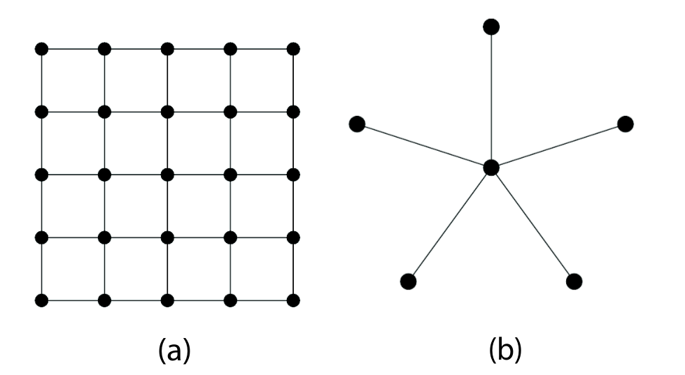
For example, consider the $D$ -dimensional square lattice of linear size $L$ , which has $L^{D}$ vertices, as shown in Fig. 1(a). The associated cluster states have symmetry-protected topological order Son et al. 2011, but they are not in TQO-1. The vertex degree is $\Delta(G)=2D$ regardless of the size of the lattice, and the maximum code distance is at most $2D+1$ , which is a constant for fixed dimension even if $L$ increases.

From above discussion, a necessary condition for a family of graph states to be in TQO-1 is that the graph degree has to be macroscopic: $\Delta(G)\in\operatorname{sublin}(n)$ . This requirement is not sufficient, however, because there are families of macroscopic-degree graphs that are not in TQO-1. Examples include the star graph and complete graph discussed in the next two sections.

Refer to caption — Figure 1: Examples of graphs that are not in TQO-1: (a) 2D regular lattice and (b) six-vertex star graph.

IV.1.2 Star graph

Consider next the star graph on $n$ vertices $K_{1,n-1}$ , as shown in Fig. 1(b), which defines GHZ states on $n$ qubits. The adjacency matrix, where the first vertex is chosen to have high degree, is

A_{1,n-1}=\begin{bmatrix}0&1&1&\cdots 1\\ 1&0&0&\cdots 0\\ \vdots&\vdots&\vdots&\cdots\vdots\\ 1&0&0&\cdots 0\end{bmatrix}.

(36)

When $i>1$ , $\text{wt}\left[\left(A_{1,n-1}\cdot\mathbf{b}^{1}\right)\vee\mathbf{b}^{1}\right]=n$ and $\text{wt}\left[\left(A_{1,n-1}\cdot\mathbf{b}^{i}\right)\vee\mathbf{b}^{i}\right]=2$ . The second of these yields $\left\{\mathbf{b}^{i}\,(i>1)\right\}\subseteq Z(G_{\rm star},n,3)$ and

Z(K_{1,n-1},n,3)^{\perp}\subseteq\left\{\mathbf{b}^{i}\,(i>1)\right\}^{\perp}=\{0^{n},\mathbf{b}^{1}\}.

However, the bitstrings $\{0^{n},\mathbf{b}^{1}\}\subseteq W(G_{\rm{star}},n,3)$ because their Hamming weights are smaller than 3. Thus, $C(K_{1,n-1},n,3)=\emptyset$ and $d^{\rm max}<3$ , and the family of star graph states is therefore not in TQO-1.

IV.1.3 Complete graph

Consider next the complete graph on $n$ vertices, $K_{n}$ , which is local-Clifford equivalent (LC-equivalent) to the star graph Van den Nest et al. 2004. An example is shown in Fig. 5(a). The adjacency matrix is $A_{K}=J-I$ , where $J$ is the matrix of all ones. In this case, $\text{wt}\left[\left(A_{K}\cdot\mathbf{b}^{i}\right)\vee\mathbf{b}^{i}\right]=n\,\forall i$ , which would imply that $d=n+1$ , an impossibility. Next consider weight-two bitstrings, corresponding to the $n-1$ independent pairings of the basis states, $\mathbf{c}^{i}=\mathbf{b}^{i}+\mathbf{b}^{i+1}$ , $i<n$ . Then $\text{wt}\left(A_{K}\cdot\mathbf{c}^{i}\right)=w\left[\left(A_{K}\cdot\mathbf{c}^{i}\right)\vee\mathbf{c}^{i}\right]=2$ , so that $\left\{\mathbf{c}^{1},\ldots,\mathbf{c}^{n-1}\right\}\subseteq Z(K_{n},n,3)$ . Only the all-zero and all-one bitstrings are orthogonal to $\mathbf{c}^{i}\;(i<n)$ , so that

Z^{\perp}(K_{n},n,3)\subseteq\left\{\mathbf{c}^{1},\ldots,\mathbf{c}^{n-1}\right\}^{\perp}=\{0^{n},1^{n}\}.

But as was the case for star graphs, both $0^{n}$ and $1^{n}$ are also in $W(K_{n},n,3)$ because $1^{n}=A_{K}\cdot\mathbf{b}^{i}+\mathbf{b}^{i}\,\forall i$ . One therefore again obtains $C(K_{n},n,3)=Z^{\perp}(K_{n},n,3)\backslash W(K_{n},n,3)=\emptyset$ , and $d^{\rm max}<3$ for the family of complete graph states. The results for the star and complete graphs are consistent with the fact that the GHZ state is not topologically ordered.

IV.2 Topologically non-trivial graph states and codes

In this section, we present some topologically non-trivial graph states and construct their associated QECCs with macroscopic distance. By embedding a classical LDPC code into the multi-star graph state, we obtain an $[[n,k,d]]$ QECC where $n=\Theta(kd)$ . Two $[[n,1,\Theta(\sqrt{n})]]$ QECCs are based on the line graphs of the complete and completely bipartite graphs, corresponding to the triangular and rook’s graph, respectively.

Despite the macroscopic distance of the QECCs presented here, it might be considered an abuse of notation to refer to them as topological codes. They do not necessarily all have local stabilizer generators, and it is not clear if the degeneracy of the code subspace has a topological origin like is the case for the 2D toric code and color code. Nevertheless, the constructions presented below are all rather simple while possessing a code distance that scales sublinearly in the number of physical qubits. Thus, we hope that these examples might be helpful in the understanding of how to construct general topological states and QECCs.

IV.2.1 Multiple copies of the star graph

Perhaps surprisingly, multiple copies of star graphs lead to a different conclusion than was found for a single copy of the star graph. Consider an $n=qm$ -vertex graph $G_{\rm{mstar}}$ composed of $q$ disconnected components, each of which is a star graph on $m$ vertices and $q\geq m$ . The adjacency matrix of this graph is block diagonal, $A_{\rm mstar}=A_{1,m-1}^{\oplus q}$ , where $A_{1,m-1}\in\mathbb{Z}_{2}^{m\times m}$ is of same form as in Eq. (36). For this family of graph states, $d^{\rm max}=m=n/q$ , which scales macroscopically with $n$ .

As in the case of a single star graph, $\text{wt}(A_{\rm mstar}\cdot\mathbf{b}^{i})=1$ and $\text{wt}\left[(A_{\rm mstar}\cdot\mathbf{b}^{i})\vee\mathbf{b}^{i}\right]=2$ when $(i\,{\rm mod}\,m)\neq 1$ , so that $\left\{\mathbf{b}^{i}|(i\,{\rm mod}\,m)\neq 1\right\}\subseteq Z(G_{\rm{mstar}},n,3)$ . Furthermore, $\left\{\mathbf{b}^{i}|i\mod m\neq 1\right\}$ is the maximum independent subset of $Z(G_{\rm{mstar}},n,m)$ , because any linear combination of these bitstrings will have maximum weight $m-1$ but each only has the first vertex as a neighbor. For any bitstring $\mathbf{k}$ with a 1 at position $i\mod m=1$ , $\text{wt}[(A\cdot\mathbf{k})\vee\mathbf{k}]\geq m$ regardless the bit value in other positions. Furthermore, all linear combinations of $\mathbf{b}^{i}$ with $(i\,{\rm mod}\,m)=1$ are orthogonal to bitstrings in $Z(G_{\rm{mstar}},n,m)$ :

Z^{\perp}(G_{\rm{mstar}},n,m)=\operatorname{span}_{\mathbb{Z}_{2}}\left\{\mathbf{b}^{i}|(i\,{\rm mod}\,m)=1\right\}.

(37)

For TQO-1, $Z^{\perp}(m)\backslash W(m)$ must not be an empty set; in the present case, we show that every bitstring in $Z^{\perp}(m)$ with Hamming weight greater or equal to $m$ is not in $W(m)$ .

Consider first the conditions where $h=A\cdot\mathbf{k}+\mathbf{l}=\mathbf{b}^{1}$ : $(A\cdot\mathbf{k})_{1}=0$ and $\mathbf{l}_{1}=1$ , and $(A\cdot\mathbf{k})_{1}=1$ and $\mathbf{l}_{1}=0$ . In both cases, $\text{wt}(\mathbf{k}\vee\mathbf{l})\geq\text{wt}(A\cdot\mathbf{k}+\mathbf{l})=1$ . Next, consider the case where $h=\mathbf{b}^{1}+\mathbf{b}^{m+1}$ . Similarly, either $(A\cdot\mathbf{k})_{m+1}=0$ and $\mathbf{l}_{m+1}=1$ , or $(A\cdot\mathbf{k})_{m+1}=1$ and $\mathbf{l}_{m+1}=0$ . Thus, $\{(A\cdot\mathbf{k})_{1},\mathbf{l}_{1},(A\cdot\mathbf{k})_{m+1},\mathbf{l}_{m+1}\}=\{1,0,1,0\},\;\{1,0,0,1\},\;\{0,1,1,0\}$ , and $\{0,1,0,1\}$ . In the first case, $(A\cdot\mathbf{k})_{1}=(A\cdot\mathbf{k})_{m+1}=1$ , so there are an odd number of indices $i\in[2,m]$ where $\mathbf{k}_{i}=1$ and an odd number of indices $j\in[m+2,2m]$ where $\mathbf{k}_{j}=1$ ; therefore $\text{wt}(\mathbf{k}\vee\mathbf{l})\geq 2$ . In the second case, there are again an odd number of indices $i\in[2,m]$ where $\mathbf{k}_{i}=1$ ; together with $\mathbf{l}_{m+1}=1$ , one again obtains $\text{wt}(\mathbf{k}\vee\mathbf{l})\geq 2$ . Likewise for the third case. Finally, $\text{wt}(\mathbf{k}\vee\mathbf{l})\geq\text{wt}(\mathbf{l})\geq 2$ in the fourth case because of $\mathbf{l}_{1}=\mathbf{l}_{m+1}=1$ . Every non-zero entry in $A\cdot\mathbf{k}+\mathbf{l}$ either requires an entry in $l$ or $\mathbf{k}$ to be non-zero. Generalizing the above argument to arbitrary linear combinations of bitstrings from $\left\{\mathbf{b}^{i}|(i\,{\rm mod}\,m)=1\right\}$ , one obtains $\text{wt}(\mathbf{k}\vee\mathbf{l})\geq\text{wt}(\mathbf{h})$ if $\mathbf{h}\in Z^{\perp}$ . Therefore, if the $\text{wt}(\mathbf{h})\geq m$ then $\text{wt}(\mathbf{k}\vee\mathbf{l})\geq m$ , i.e. $\mathbf{h}\notin W(m)$ ; thus $C(G_{\rm mstar},n,m)\neq\emptyset$ .

Increasing $d$ to $m+1$ would result in $\mathbf{b}^{i}\in Z(G_{\rm{mstar}},n,m+1)$ when $i=1\mod m$ , because $\text{wt}(A\cdot\mathbf{b}^{i}\vee\mathbf{b}^{i})=m\leq m+1$ . In that case, every basis bitstring is in $Z(m+1)$ so that $Z^{\perp}(m+1)=\{0^{n}\}$ and $C(m+1)=\emptyset$ . One therefore concludes that for the family of multi-star graph states, $d^{\rm max}=m$ . If $q=\Theta(m)$ , then $d^{\rm max}=\Theta(\sqrt{n})$ and this family of graph states is in TQO-1. The same conclusion evidently also holds for multiple copies of complete graphs.

In summary, for an $n=qm$ -vertex multi-star graph, composed of $q$ disconnected $m$ -vertex star graphs ( $q\geq m$ ):

	$\displaystyle C(G_{\rm mstar},n,m)$	$\displaystyle=$	$\displaystyle\{\mathbf{h}\in\operatorname{span}_{\mathbb{Z}_{2}}\left\{\mathbf{b}^{i}\|(i\,{\rm mod}\,m)=1\right\}$		(38)
			$\displaystyle\quad\|\text{wt}(\mathbf{h})\geq m\}.$		(38)

Combining this result with Corollary 2, one can construct a $[[qm,\Theta(q),m]]$ QECC using a classical LDPC code. Suppose one is given a classical linear code $\mathtt{C}=[q,c_{1}q,c_{2}q]$ , where $c_{1}$ and $c_{2}$ are constant and $c_{2}q\geq m$ . Each codeword in this classical code are mapped to a logical state in a QECC in the following way:

	$\displaystyle\mathbf{h}\in\mathtt{C}\subseteq\{0,1\}^{q}$	$\displaystyle\mapsto$	$\displaystyle r(\mathbf{h})=\sum_{i\in[q]}\mathbf{h}_{i}\mathbf{b}^{1+m(i-1)}\in\set{0,1}^{n}$		(39)
		$\displaystyle\mapsto$	$\displaystyle\Ket{r(\mathbf{h})}_{G_{\rm mstar}}\in\mathscr{H}_{2}^{\otimes n}.$		(39)

As the Hamming weight of every bitstring in $\mathtt{C}$ is no less than $c_{2}q$ , every $r(\mathbf{h})$ mapped from the classical code also has Hamming weight no less than $c_{2}q$ .

Theorem 3.

Subspace $\operatorname{span}_{\mathbb{C}}\{\Ket{r(\mathbf{h})}_{G_{\rm mstar}}\}$ is a $[[qm,c_{1}q,m]]$ QECC.

Proof.

From Corollary 2, one only need show that the following conditions hold for all $\mathbf{h}\neq\mathbf{h}^{\prime}\in\mathtt{C}$ :

	$\displaystyle r(\mathbf{h})\in C(G_{\rm mstar},n,m);$		(40)
	$\displaystyle r(\mathbf{h})+{r(\mathbf{h}^{\prime})}\notin W(G_{\rm mstar},n,m).$		(41)

Following the arguments presented in Sec. IV.2.1, Eq. 40 holds because $r(\mathbf{h})$ is a linear combination of $\left\{\mathbf{b}^{i}|(i\,{\rm mod}\,m)=1\right\}$ . In the classical LDPC code $\mathtt{C}$ , one has $\text{wt}(h+\mathbf{h}^{\prime})\geq c_{2}q$ for every $h,\mathbf{h}^{\prime}\in\mathtt{C}$ . Therefore,

\text{wt}(r(\mathbf{h})+r(\mathbf{h}^{\prime}))\geq c_{2}q,\forall\mathbf{h},\mathbf{h}^{\prime}\in\mathtt{C},

(42)

leading to Eq. (41). ∎

IV.2.2 Toric graph

The toric graph is a $2L^{2}$ -vertex graph representing a graph state, and is LC-equivalent to one of the ground states in the toric code Liao and Feder 2021. The toric graph state is in TQO-1 because the toric code has macroscopic distance $d=L\in O(\sqrt{n})$ . Nevertheless, it might be helpful to the reader to confirm this result using the method discussed in this work, by showing that set $C(G_{\rm toric},2L^{2},L)$ is non-empty. The qubits in the 2D toric code are placed on the edges of a square $L\times L$ lattice. Qubits are labelled by $(i,j,d)\in[L]\times[L]\times\{x,y\}$ , where $(i,j)$ are the spatial coordinates and $x$ and $y$ denote the orientation of the qubit on horizontal or vertical edges. The adjacency matrix of the toric graph is Liao and Feder 2021

$\displaystyle A_{ijd_{1},lmd_{2}}$	$\displaystyle=$	$\displaystyle\delta_{d_{1},x}\delta_{d_{2},x}\delta_{m,j}(\delta_{l,L}\theta_{i,L-1}+\delta_{i,L}\theta_{l,L-1})$	(43)
	$\displaystyle+$	$\displaystyle\delta_{d_{1},y}\delta_{d_{2},y}\delta_{m,j}(\delta_{i,1}\theta_{2,l}+\delta_{l,1}\theta_{2,i})$
	$\displaystyle+$	$\displaystyle\delta_{d_{1},y}\delta_{d_{2},x}(\delta_{m,j}+\delta_{m-1,j})\theta_{l,i-1}\theta_{2,i}$
	$\displaystyle+$	$\displaystyle\delta_{d_{1},x}\delta_{d_{2},y}(\delta_{m,j}+\delta_{j-1,m})\theta_{i+1,l}\theta_{i,L-1},\hphantom{aa}$

where $\delta_{i,j}$ and $\theta_{i,j}$ are the usual Kronecker and Heaviside theta functions, respectively:

\delta_{i,j}=\begin{cases}1&j=i\\ 0&{\rm otherwise}\end{cases}\;{\rm and}\;\theta_{i,j}=\begin{cases}1&i\leq j\\ 0&{\rm otherwise}.\end{cases}

(44)

While it might not be immediately apparent from the form of the adjacency matrix, the toric graph in fact corresponds to multiple copies of the star graph, which are then connected by half graphs Liao and Feder 2021, as shown in Fig. 3. Appendix D shows that

C(G_{\rm toric},2L^{2},L)=\left\{\sum_{j=1}^{L}\mathbf{b}^{Ljx},\sum_{i=1}^{L}\mathbf{b}^{1jy},\sum_{i=1}^{L}(\mathbf{b}^{Ljx}+\mathbf{b}^{1jy})\right\}.

(45)

These three bitstrings correspond to the three graph basis states that are LC-equivalent to the logical states of the toric code. Together with the toric graph state itself (the zero state in this representation), they span a subspace that is locally equivalent to the 2D toric code.

IV.2.3 Connected multiple star graphs

Given that both multiple star graphs and the toric graph (multiple star graphs connected via half graphs) are in TQO-1, one might wonder if any connected graph $G_{\rm cmstar}$ that is formed by a regular linking of multiple star graphs is also in TQO-1. It turns out that this is in fact the case, as is proven here. An example $G_{\rm cmstar}$ is depicted in Fig. 4.

As was the case for the toric graph, label the vertices as $(i,j,d)\in[L]\times[L]\times\{x,y\}$ . There are $2L(L-1)$ vertices in the middle two layers that are labelled by $[2,L]\times[L]\times\{y\}$ and $[L-1]\times[L]\times\{x\}$ . As the corresponding vertices have constant degree $\text{wt}(A\cdot\mathbf{b}^{ijd})$ (which is 3 in the example shown in Fig. 4), one obtains $\mathbf{b}^{ijd}\in Z(G_{\rm cmstar},2L^{2},L)$ if $(i,j,d)\in[2,L]\times[L]\times\{y\}\cup[L-1]\times[L]\times\{x\}$ . On the other hand, the neighborhood of vertices $(1,i,y)$ and $(L,j,x)$ , $i,j\in[L]$ , is composed of $L-1$ vertices, and each of these neighborhoods is disjoint. As a result, if bitstring $\mathbf{k}$ has non-zero entry at $(1,i,y)$ or $(L,j,x)$ , then $\text{wt}(\mathbf{k}\vee A\mathbf{k})\geq L$ and so $\mathbf{b}^{1iy},\mathbf{b}^{Ljx}\notin Z(G_{\rm cmstar},2L^{2},L)$ for every $i,j\in[L]$ . Thus $Z^{\perp}(L)=\operatorname{span}\{\mathbf{b}^{11y},\cdots,\mathbf{b}^{1Ly},\mathbf{b}^{L1x},\cdots,\mathbf{b}^{LLx}\}$ and

\left\{\sum_{j=1}^{L}\mathbf{b}^{Ljx},\sum_{i=1}^{L}\mathbf{b}^{1jy},\sum_{i=1}^{L}(\mathbf{b}^{Ljx}+\mathbf{b}^{1jy})\right\}\subseteq Z^{\perp}(L).

(46)

These three bitstrings are not in $W(L)$ for reasons similar to those discussed in Sec. (IV.2.1), so one obtains the result that $C(G_{\rm cmtar},2L^{2},L)\neq\emptyset$ and the family of connected multi-star states is also in TQO-1.

IV.2.4 Line graph of the complete graph

One of the distinguishing features of the previous two examples, multiple copies of the star graph and the toric graph, is that the maximum vertex degree (the maximum value of the vertex degree taken over all vertices) increases with the total number of vertices. Evidently the examples of a single copy of the star and complete graph show that this condition is not sufficient for a family of graphs to be in TQO-1. It is nevertheless worthwhile to consider other examples of graphs with this behaviour. One candidate is the line graph of the complete graph, $L(K_{m})$ , also known as the triangular graph $T_{m}$ , considered here. An example of a complete graph and its triangular graph are depicted in Fig. 5.

The graph $K_{m}=(V,E)$ is the $m$ -vertex complete graph where each pair of vertices shares an edge, so the number of edges is $|E|=\binom{m}{2}={m(m-1)}/{2}$ . The line graph of $K_{m}$ is $L(K_{m})=T_{m}=(V^{\prime},E^{\prime})$ ; by definition, $|V^{\prime}|=|E|=n$ ; the number of edges is $|E^{\prime}|=2(m-2)$ . The adjacency matrices of $K_{m}$ and $T_{m}$ are denoted $A\in\mathbb{Z}_{2}^{m\times m}$ and $A^{\prime}\in\mathbb{Z}_{2}^{n\times n}$ , respectively. The main result in this section is Theorem 4, which is proven by showing that the set $C(T_{m},\binom{m}{2},\lfloor m/2\rfloor)$ is non-empty for all $2\leq m\in\mathbb{N}$ .

Theorem 4.

The family of line graph states $\mathtt{S}=\Set{\Ket{T_{m}}}_{m\geq 2}$ is in TQO-1.

Proof.

A full proof is given in Appendix E, but the main ideas are sketched here. Consider a bitstring $\mathbf{s}^{v}\in\set{0,1}^{|E|}$ , which only has non-zero entries at edges incident to vertex $v$ in graph $K_{m}$ . From the construction of the line graph, the column vector of the adjacency matrix $A^{\prime}\cdot\mathbf{b}^{e_{ij}}$ only has non-zero entries at edges incident to either $v_{i}$ or $v_{j}$ (except for $e_{ij}$ itself), which are formally expressed as $A^{\prime}\cdot\mathbf{b}^{e_{ij}}=\mathbf{s}^{v_{i}}+\mathbf{s}^{v_{j}}$ ; then

A^{\prime}\cdot\mathbf{k}=\sum_{e_{ij}}\mathbf{k}_{e_{ij}}(A^{\prime}\cdot\mathbf{b}^{e_{ij}})=\sum_{e_{ij}}\mathbf{k}_{e_{ij}}(\mathbf{s}^{v_{i}}+\mathbf{s}^{v_{j}}).

(47)

The sum (bitwise XOR) of $\mathbf{s}^{v}$ over edges are equivalently expressed as a sum over a subset of vertices

A^{\prime}\cdot\mathbf{k}=\sum_{v\in V_{\mathbf{k}}^{\rm o}}\mathbf{s}^{v},

(48)

where $V_{\mathbf{k}}^{\rm o}$ is the subset of vertices with odd degree in subgraph $(K_{m})_{\mathbf{k}}$ . Using this relation, one can obtain the Hamming weight $\text{wt}(A^{\prime}\cdot\mathbf{k})=l_{\mathbf{k}}(m-l_{\mathbf{k}})$ , where $l_{\mathbf{k}}=|V_{\mathbf{k}}^{\rm{o}}|$ . Next, one can show that $\text{wt}(A^{\prime}\cdot\mathbf{k})<\lfloor m/2\rfloor$ only if $l_{\mathbf{k}}=0$ , i.e. that all the vertices in subgraph $(K_{m})_{\mathbf{k}}$ have even degree. As a result, every bitstring $\mathbf{k}$ in $Z(T_{m},\binom{m}{2},\lfloor m/2\rfloor)$ corresponds to a subgraph $(K_{m})_{\mathbf{k}}$ that is an Eulerian cycle or sum (edge symmetric difference) of Eulerian cycles. Because of the special structure of the complete graph, every cycle in $K_{m}$ can be decomposed into a sum of triangles, which allows for the determination of a maximum independent subset of $Z(\lfloor m/2\rfloor)$ with every member a bitstring corresponding to a triangle; furthermore, the bitstring $\mathbf{s}^{v}$ can be shown to be orthogonal to all of these bitstrings, so that $\mathbf{s}^{v}\in Z^{\perp}(T_{m},\binom{m}{2},\lfloor m/2\rfloor)$ for every $v\in V$ . Finally, using standard algebraic arguments, one can prove that $\mathbf{s}^{v}\notin W^{\perp}(T_{m},\binom{m}{2},\lfloor m/2\rfloor)$ , so that $\mathbf{s}^{v}\in C(T_{m},\binom{m}{2},\lfloor m/2\rfloor)$ for every $v\in V$ . Given that $C(T_{m},\binom{m}{2},\lfloor m/2\rfloor)\neq\emptyset$ and the code distance is macroscopic, the family of line graphs of the complete graph is in TQO-1. ∎

Because of Lemma 4 and $\mathbf{s}^{v_{1}}\in C(L(K_{m}),\binom{m}{2},\lfloor m/2\rfloor)$ , the following result holds:

Corollary 3.

Subspace $\operatorname{span}_{\mathbb{C}}\Set{\Ket{L(K_{m})},\Ket{\mathbf{s}^{v_{1}}}_{L(K_{m})}}$ is a $[\binom{m}{2},1,\lfloor m/2\rfloor]$ QECC.

An immediate question is: is it possible to expand this code using Corollary 2, so that it can encode more than one logical qubit while simultaneously keeping the same code distance $d=\lfloor m/2\rfloor$ . It turns out that this is not possible, unfortunately. Given that $C(L(K_{m}),\binom{m}{2},\lfloor m/2\rfloor)$ contains more than one bitstring, one would be tempted to choose another one, for example $\mathbf{s}^{v_{2}}$ , so that

\operatorname{span}_{\mathbb{C}}\Set{\Ket{L(K_{m})},\Ket{\mathbf{s}^{v_{1}}}_{L(K_{m})},\Ket{\mathbf{s}^{v_{2}}}_{L(K_{m})}}

is also a QECC with distance $d=\lfloor m/2\rfloor$ . However, from Corollary 2, for the expanded three-dimensional subspace to be a QECC with $d=\lfloor m/2\rfloor$ , $\mathbf{s}^{v_{2}}$ needs to be in $Z^{\perp}(\lfloor m/2\rfloor)$ while $\mathbf{s}^{v_{1}}+\mathbf{s}^{v_{2}}$ cannot be in $W$ . The second condition does not hold because $\mathbf{s}^{v_{1}}+\mathbf{s}^{v_{2}}$ is one of the column vectors of the adjacency matrix $A^{\prime}$ . For any other bitstring $\mathbf{h}\in C(L(K_{m}),\binom{m}{2},\lfloor m/2\rfloor)$ , similar problems will be present, so that it is not possible to expand $\operatorname{span}_{\mathbb{C}}\{\Ket{L(K_{m})},\Ket{\mathbf{s}^{v_{1}}}_{L(K_{m})}\}$ to encode more logical qubits without sacrificing the code distance.

IV.2.5 Line graph of the complete bipartite graph

The second example considered here is similar to the first one: the graph state represented by the line graph of the balanced complete bipartite graph $L(K_{m,m})$ , which is also called a rook’s graph because the edges represent all the possible moves a rook can take in the game of chess. An example of a complete bipartite graph and its associated rook’s graph are depicted in Fig. 6.

The complete bipartite graph $K_{m,m}$ has $2m$ vertices divided into two complementary subsets of the same size $V=X\sqcup Y=\set{v^{x}_{1},\ldots,v_{m}^{x}}\sqcup\set{v^{y}_{1},\ldots,v_{m}^{y}}$ . Similarly, $V,E,A$ denote the set of vertices, the set of edges, and the adjacency matrix of $K_{m,m}$ , respectively, while $V^{\prime},E^{\prime},A^{\prime}$ are used for the line graph $L(K_{m,m})$ . In $K_{m,m}$ , every vertex in the set $X$ is connected to every vertex in the $Y$ , but there are no edges connecting two vertices in $X$ or two vertices in $Y$ ; there are therefore $m^{2}$ edges in total: $|E|=m^{2}$ and $|V^{\prime}|=n=m^{2}$ .

The main result of this section is Theorem 5, which is proven by showing that $C(L(K_{m,m}),m^{2},m)\neq\emptyset$ :

Theorem 5.

The family of line graph states $\mathtt{S}=\Set{\Ket{L(K_{m,m})}}_{m\geq 4}$ is in TQO-1.

Proof.

Again, only a sketch of the proof is provided here, and the full proof is found in Appendix F. Analogously, $\mathbf{s}^{v}$ represents the bitstring that only has non-zero entries at edges incident to $v$ in graph $K_{m,m}$ . The column vector $A^{\prime}\cdot\mathbf{b}^{e}$ , where $e=(v_{i}^{x},v_{j}^{y})$ , only has non-zero entries at edges incident to either $v_{i}^{x}$ or $v_{j}^{y}$ , so that $A^{\prime}\cdot\mathbf{b}^{e}=\mathbf{s}^{v_{i}^{x}}+\mathbf{s}^{v_{j}^{y}}$ . Similarly, $A^{\prime}\cdot\mathbf{k}=\sum_{v\in V_{\mathbf{k}}^{\rm o}}\mathbf{s}^{v}$ , where $V_{\mathbf{k}}^{\rm{o}}$ can be partitioned into two complementary sets $V_{\mathbf{k}}^{\rm o}=X_{\mathbf{k}}^{\rm o}\cup Y_{\mathbf{k}}^{\rm o}$ . Using this expression, one can calculate the Hamming weight of $\text{wt}(A^{\prime}\cdot\mathbf{k})=(l_{\mathbf{k}}^{x}+l_{\mathbf{k}}^{y})m-2l_{\mathbf{k}}^{x}l_{\mathbf{k}}^{y}$ , where $l_{\mathbf{k}}^{x}=|X_{\mathbf{k}}^{\rm o}|$ and $l_{\mathbf{k}}^{y}=|Y_{\mathbf{k}}^{\rm o}|$ . With this in hand, one obtains $\text{wt}[(A^{\prime}\cdot\mathbf{k})\vee\mathbf{k})]<m$ only if $l_{\mathbf{k}}^{x}=l_{\mathbf{k}}^{y}=0$ by a simple algebraic argument, i.e. all the vertices in subgraph $(K_{m,m})_{\mathbf{k}}$ has even degree.

According to Euler’s theorem, every bitstring in $Z\left(L(K_{m,m}),n,m\right)$ corresponds to an Eulerian cycle or sum (edge symmetric difference) of Eulerian cycles. Furthermore, because of the special structure of $K_{m,m}$ , every cycle in $K_{m,m}$ can be decomposed into the sum of 4-edge cycles so that a maximum independent subset of $Z(m)$ are chosen where each bitstring corresponds to a 4-edge cycle. Proving that $\mathbf{s}^{v}$ is orthogonal to every bitstring corresponding to $4$ -edge cycles, one obtains the set $\mathbf{s}^{v}\in Z^{\perp}(m)$ for every $v\in V$ . Finally, one can prove $\mathbf{s}^{v}\notin W(m)$ by some algebraic arguments, so that $\mathbf{s}^{v}\in C(m)$ for every $v\in V$ . ∎

For the graph state represented by the line graph of the complete bipartite graph, the following result holds from Lemma 4 and the fact that $\mathbf{s}^{v}\in C(L(K_{m,m}),m^{2},m)$ :

Corollary 4.

The subspace

\operatorname{span}_{\mathbb{C}}\Set{\Ket{L(K_{m,m})},\Ket{\mathbf{s}^{v}}_{L(K_{m,m})}}

is a $[m^{2},1,m]$ QECC.

The line graph $L(K_{m,m})$ resembles $L(K_{m})$ in this respect, and the corresponding graph state suffers a similar expansion problem; it is not possible to expand this code without decreasing the code distance.

V 3D toric graph code

In this section we first present the structure of a generalized toric graph. A family of $[[n,n^{1/3},n^{1/3}]]$ QECCs with geometrically local stabilizers is then obtained. This is considered as a generalization of toric code, and is referred as a 3D toric graph code in this work.

In the toric code, qubits are divided into two complementary subsets $X\cup Y$ , corresponding to their placement on horizontal and vertical edges of the two-dimensional lattice, respectively. In the associated toric graph, the induced subgraphs in $X$ and $Y$ separately are comprised of multiple star graphs, while the subgraph connecting $X$ and $Y$ are half graphs. One can consider the toric graph to have a two-layer structure: each layer is an $L^{2}$ -vertex multi-star graph, and different layers are connected by half graphs. It is natural to extend this two-layer structure to $L$ layers. In this way one obtains an $L^{3}$ -vertex generalized toric graph $G_{\rm gtoric}$ . Vertices are denoted by $(i,j,k)\in[L]^{3}$ , where $i,j,k\in[L]$ .

The adjacency matrix of the generalized toric graph $G_{\rm gtoric}$ is a straightforward generalization of Eq. (43):

	$\displaystyle A_{i_{1}j_{1}k_{1},i_{2}j_{2}k_{2}}$	(49)
$\displaystyle=$	$\displaystyle\delta_{j_{1},j_{2}}\delta_{k_{1},k_{2}}\left(\delta_{i_{1},1}\theta_{2,i_{2}}+\delta_{i_{2},1}\theta_{2,i_{1}}\right)$
$\displaystyle+$	$\displaystyle\delta_{j_{1}j_{2}}(\delta_{k_{1},k_{2}+1}\theta_{i_{2},i_{1}}\theta_{2,i_{2}}+\delta_{k_{2},k_{1}+1}\theta_{i_{1},i_{2}}\theta_{2,i_{1}})$
$\displaystyle+$	$\displaystyle\delta_{j_{1},j_{2}+1}\delta_{k_{1},k_{2}+1}\theta_{i_{2},i_{1}}\theta_{2,i_{2}}$
$\displaystyle+$	$\displaystyle\delta_{j_{2},j_{1}+1}\delta_{k_{2},k_{1}+1}\theta_{i_{1},i_{2}}\theta_{2,i_{1}},$

where $i_{1},i_{2},j_{1},j_{2},k_{1},k_{2}\in[L]$ . Similar to the $2L^{2}$ -vertex toric graph, the vertices in $G_{\rm gtoric}$ can be partitioned into $L$ disjoint subsets $X_{1}\cup\cdots\cup X_{L}$ of the same size $L^{2}$ , where $X_{i}=[L]\times[L]\times\{i\}$ . The induced subgraphs on $X_{i}$ are also composed of multiple star graphs and $X_{i}$ and $X_{i+1}$ are connected by half graphs, similar to $X$ and $Y$ in the toric graph.

Theorem 6.

The family of generalized toric graph state $\mathtt{S}=\Set{\Ket{G_{\rm gtoric}}\in\mathscr{H}_{2}^{\otimes L^{3}}}_{L\in\mathbb{N}}$ is in class TQO-1.

The graph state $\Ket{G_{\rm gtoric}}\in\mathscr{H}_{2}^{\otimes L^{3}}$ is topologically ordered, as stated in Theorem 6. The proof that $\Set{\Ket{G_{\rm gtoric}}}$ is in TQO-1 takes a different approach than was pursued in previous sections (i.e. via showing that $d^{\rm max}\in\operatorname{sunlin}(n)$ ). Rather, $G_{\rm gtoric}$ is a generalization of the toric graph, and recall that the toric graph state is LC-equivalent to one of the ground states in 2D toric code. We show that it is possible to construct a generalized toric code such that $\Ket{G_{\rm gtoric}}$ is (or is LC-equivalent to) one of the states in this code. Next, we present the construction of an $[[L^{3},L,L]]$ QECC with growing distance, a large number of logical qubits, and local stabilizer generators, using the generalized toric graph state.

From the adjacency matrix Eq. (49), one readily obtains the stabilizer generators of the generalized toric graph state $\Ket{G_{\rm gtoric}}$ :

$\displaystyle S_{1jk}$	$\displaystyle:=$	$\displaystyle X_{1jk}\prod_{l=2}^{L}Z_{ljk};$	(50)
$\displaystyle S_{ijk}$	$\displaystyle:=$	$\displaystyle X_{ijk}Z_{1jk}\left(\prod_{l=i}^{L}Z_{lj,k+1}\right)\left(\prod_{l=2}^{i}Z_{lj,k-1}\right)$	(51)
	$\displaystyle\times$	$\displaystyle\left(\prod_{l=i}^{L}Z_{l,j+1,k+1}\right)\left(\prod_{l=2}^{i}Z_{l,j-1,k-1}\right),i\geq 2,\hphantom{aa}$	(51)

which act on $L$ and $2L$ qubits, respectively. First, transform the non-local stabilizer generators of $\Ket{G_{\rm gtoric}}$ to a set of local but not all independent stabilizers. Let $B=\set{1}\times[L]\times[L]$ denote the subset of qubits labeled by $i=1$ and $H_{B}$ denote the Hadamard gate acting on the qubits in $B$ :

H_{B}=\prod_{j,k\in[L]}H_{1jk}.

(52)

Lemma 7.

The state $H_{B}\Ket{G_{\rm gtoric}}$ is stabilized by

	$\displaystyle S_{ijk}^{\prime\prime}=$	$\displaystyle X_{ijk}X_{i+1,j,k}Z_{i,j,k+1}Z_{i,j+1,k+1}$
		$\displaystyle\times Z_{i+1,j,k-1}Z_{i+1,j-1,k-1}~{\rm mod}~L$		(53)

for all $i,j,k\in[L]$ .

Proof.

Multiplying neighboring stabilizer generators, one obtains a new set of local stabilizer generators:

•

$2\leq i\leq L-1$ :

		$\displaystyle S_{ijk}^{\prime}=S_{ijk}S_{i+1,jk}$		(54)
	$\displaystyle=$	$\displaystyle X_{ijk}X_{i+1,j,k}Z_{i,j,k+1}Z_{i,j+1,k+1}Z_{i+1,j,k-1}Z_{i+1,j-1,k-1};$

•

$i=1$ :

	$\displaystyle S_{1jk}^{\prime}=$	$\displaystyle S_{2jk}S_{1,j,k+1}S_{1,j+1,k+1}$		(55)
	$\displaystyle=$	$\displaystyle X_{2jk}Z_{1jk}Z_{2,j-1,k-1}Z_{2,j,k-1}X_{1,j,k+1}X_{1,j+1,k+1};$

•

$i=L$ :

	$\displaystyle S_{Ljk}^{\prime}=$	$\displaystyle S_{Ljk}S_{1,j,k-1}S_{1,j-1,k-1}$		(56)
	$\displaystyle=$	$\displaystyle X_{Ljk}Z_{1jk}Z_{L,j,k+1}Z_{L,j+1,k+1}X_{1,j,k-1}X_{1,j-1,k-1}.$

These $S^{\prime}_{ijk}$ stabilize the state $\Ket{G_{\rm gtoric}}$ , but they are not all expressed as the same combination of Pauli operators. Because $HXH=Z$ and $HZH=X$ , applying the Hadamard conjugation $S^{\prime\prime}_{ijk}=H_{B}S^{\prime}_{ijk}H_{B}$ one obtains

$\displaystyle S_{1jk}^{\prime\prime}=$	$\displaystyle X_{1jk}X_{2jk}Z_{1,j,k+1}Z_{1,j+1,k+1}Z_{2,j-1,k-1}Z_{2,j,k-1},$	(57)
$\displaystyle S_{Ljk}^{\prime\prime}=$	$\displaystyle X_{Ljk}X_{1jk}Z_{L,j,k+1}Z_{L,j+1,k+1}Z_{1,j,k-1}Z_{1,j-1,k-1},$	(58)
$\displaystyle S_{ijk}^{\prime\prime}=$	$\displaystyle S_{ijk}^{\prime},2\leq i\leq L-1,$	(59)

which is translationally invariant, subject to the condition that all indices of Pauli operators are evaluated modulo $L$ . ∎

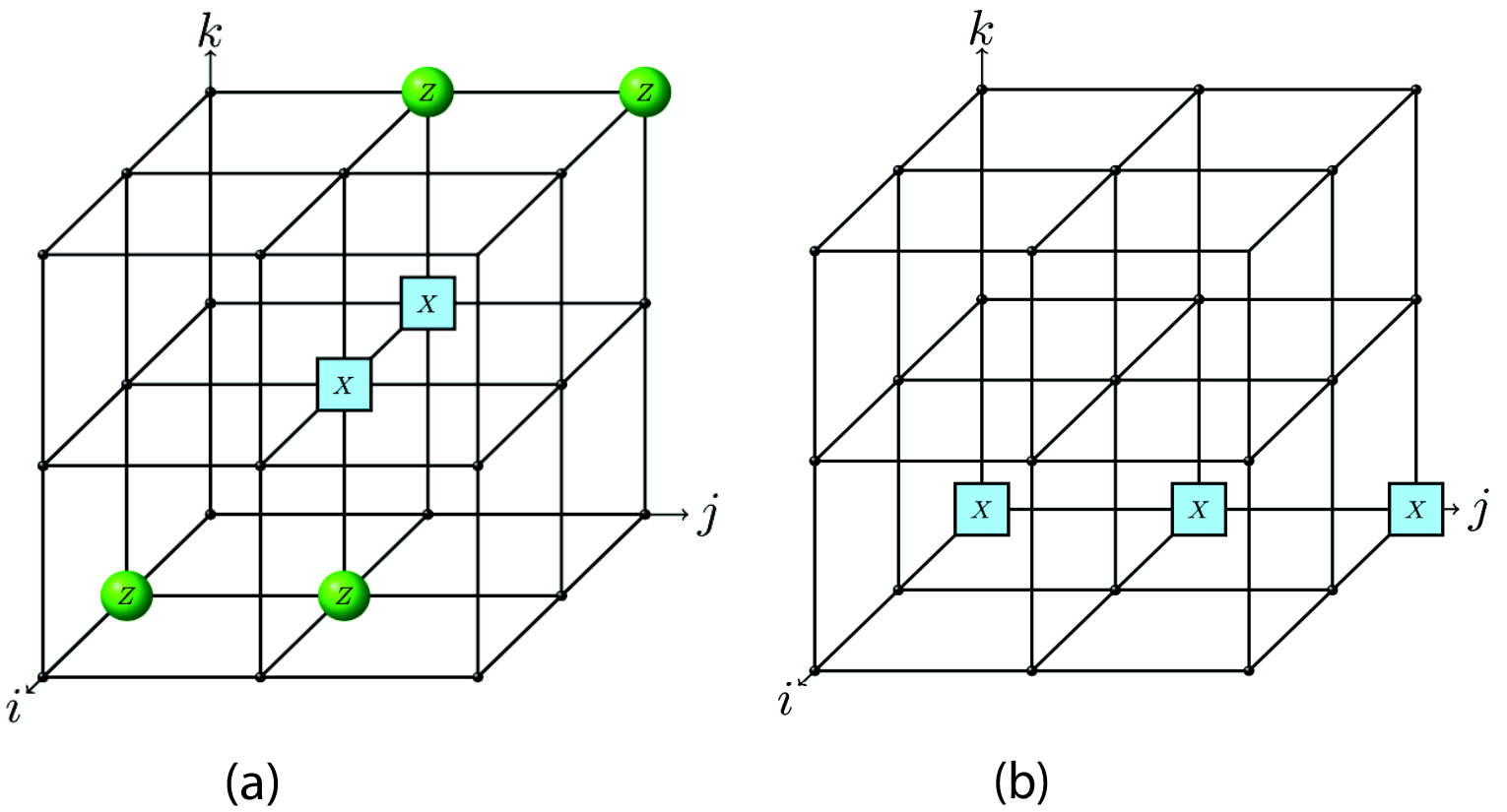
Thus, the physical qubits can be arranged on the vertices of a three-dimensional lattice subject to periodic boundary conditions, i.e. a 3-torus, and the stabilizer generators are six-local. The geometry and stabilizers $S_{ijk}^{\prime\prime}$ are shown in Fig. 7(a) .

Theorem 7.

The subspace $C_{\rm T}\subseteq\mathscr{H}_{2}^{\otimes L^{3}}$ stabilized by $\{S_{ijk}^{\prime\prime}\}$ is an $[[L^{3},L,L]]$ stabilizer QECC.

This result is rigorously proven in Appendix G. There are some known 3D codes that share a similar scaling in the distance and the number of logical qubits with this 3D toric graph code. For example, the ground-state subspace of the X-cube model Vijay et al. 2016, with qubits on the edges of an $L\times L\times L$ 3D lattice, is a $[[3L^{3},6L-3,\Omega(L)]]$ stabilizer QECC (this scaling is in contrast with that of the 3D toric code Castelnovo and Chamon 2008 which has a similar geometry, but which is a $[[3L^{3},3,L]]$ QECC); the Chamon model defined on a $2L\times 2L\times 2L$ lattice is a $[[4L^{3},4L,\Omega(L)]]$ stabilizer QECC Bravyi et al. 2011; and the Checkerboard model Shirley et al. 2019 is locally equivalent to two copies of the X-cube model. Haah’s cubic code Haah 2011 has two qubits on each vertex, and has a growing number of logical qubits and macroscopic distance, neither of which unfortunately cannot be calculated easily.

VI Conclusions

In this work, we derive a set of necessary and sufficient conditions for a family of graph states to be topologically ordered under the definition of TQO-1 in Sec. III. Using the derived criteria, we provide various pertinent examples in Sec. IV; we show that graphs with constant vertex degree and the star and complete graphs are not in TQO-1 in Sec. IV.1, whereas the toric graph, multiple star graph, connected multiple star graph, the line graphs of the complete and the line graphs of complete bipartite graphs are in TQO-1 (shown in Sec. IV.2). Lastly, by generalizing the toric graph obtained from the 2D toric code, we developed a topological code with qubits on the vertices of a three-torus in Sec. V, with six-local stabilizers. The code distance and the number of logical qubits both scale as $n^{1/3}$ , where $n$ is the number of qubits.

The line graphs of the complete and the line graphs of complete bipartite graphs are chosen because they are both strongly regular graphs with vertex degree that grows with the total number of vertices, and not because their connectivity is necessarily simple to generate in practice; in fact, they are unlikely to be related to stabilizer codes with geometrically local operators. These families are relatively straightforward to analyze at the cost of being somewhat artificial; whether they are related to any known topological codes Dua et al. 2019 would is unknown. In addition, the 3D toric graph code developed in this paper has similar behaviors to some cubic codes, such as the X-cube model and the Chamon model and their relation would be an interesting avenue for future investigation.

The potential of this graph-theoretic framework has not been fully exploited. For example, is there a signature in the graph connectivity that could allow the construction of improved LDPC codes, i.e. where the number of encoded qubits and the code distance scales better than $n^{1/3}$ , where $n$ is the number of physical qubits? In the current formalism there is no presumption of geometric locality; on the one hand this allows for the consideration of a wide range of graph families, but on the other could make a physical implementation of the code potentially daunting. Another fruitful line of inquiry is: can the criteria for TQO-1 developed here be used to determine if a given code is self-correcting? We hope to address these and related questions in future work.

Acknowledgements.

This work was supported by the Natural Sciences and Engineering Research Council of Canada and the Major Innovation Fund of the Government of Alberta.

Appendix A Stabilized subspace

Remark.

Proof.

If $\operatorname{span}_{\mathbb{C}}\{\Ket{G},\Ket{\psi}\}$ is a stabilized subspace, one can always choose $n-1$ independent and commuting stabilizers $\Set{S^{\prime}_{1},\ldots,S^{\prime}_{n-1}}$ satisfying

\displaystyle S^{\prime}_{i}\Ket{G}=\Ket{G},S^{\prime}_{i}\Ket{\psi}=\Ket{\psi}\forall i\in[n-1].

(60)

State $\Ket{G}$ is a stabilizer state, so there exists an element $S_{n}^{\prime}$ independent of $\Set{S^{\prime}_{1},\ldots,S^{\prime}_{n-1}}$ which commutes with every $S_{i}^{\prime}(i\in[n-1])$ , such that $S_{n}^{\prime}\Ket{G}=\Ket{G}$ . As commuting operators share eigenstates and the eigenvalues of $S_{n}^{\prime}$ are $\pm 1$ , either $S_{n}^{\prime}\Ket{\psi}=\Ket{\psi}$ or $S_{n}^{\prime}\Ket{\psi}=-\Ket{\psi}$ . Because $S_{n}^{\prime}\Ket{\psi}=\Ket{\psi}$ leads to $\Ket{\psi}=\Ket{G}$ , contradicting the fact that $\Ket{G}$ and $\Ket{\psi}$ are orthogonal, one must conclude that $S_{n}^{\prime}\Ket{\psi}=-\Ket{\psi}$ .

As the graph state $\Ket{G}$ is also stabilized by the $\{S_{i}\}_{i\in[n]}$ from Eq. (18), one can transform the stabilizer generator set $\Set{S_{i}^{\prime}}_{i\in[n]}$ to $\Set{S_{i}}_{i\in[n]}$ using an invertible matrix $R\in\mathbb{Z}_{2}^{n\times n}$ :

S_{i}=\prod_{j=1}^{n}{S_{j}^{\prime}}^{R_{ij}},i\in[n],

(61)

where ${S_{j}^{\prime}}^{0}=\mathds{1}$ . With Eq. (60) and $S_{n}^{\prime}\Ket{\psi}=-\Ket{\psi}$ , one obtains

	$\displaystyle S_{i}\Ket{\psi}=$	$\displaystyle\prod_{j=1}^{n}{S_{j}^{\prime}}^{R_{ij}}\Ket{\psi}={S_{n}^{\prime}}^{R_{in}}\Ket{\psi}$		(62)
	$\displaystyle=$	$\displaystyle(-1)^{R_{in}}\Ket{\psi}\forall i\in[n].$

The graph basis state $\Ket{\mathbf{h}}_{G}$ , where $\mathbf{h}\in\set{0,1}^{n}$ and $h_{i}=R_{in}$ for every $i\in[n]$ , also satisfies

$\displaystyle S_{i}\Ket{\mathbf{h}}_{G}=$	$\displaystyle X_{i}\prod_{(i,j)\in E}Z_{j}Z_{1}^{\mathbf{h}_{1}}\otimes Z_{2}^{\mathbf{h}_{2}}\otimes\cdots\otimes Z_{n}^{\mathbf{h}_{n}}\Ket{G}$
$\displaystyle=$	$\displaystyle(-1)^{\mathbf{h}_{i}}Z_{1}^{\mathbf{h}_{1}}\otimes Z_{2}^{\mathbf{h}_{2}}\otimes\cdots\otimes Z_{n}^{\mathbf{h}_{n}}X_{i}\prod_{(i,j)\in E}Z_{j}\Ket{G}$
$\displaystyle=$	$\displaystyle(-1)^{\mathbf{h}_{i}}\Ket{\mathbf{h}}_{G}=(-1)^{R_{in}}\Ket{\mathbf{h}}_{G}.$	(63)

Therefore, $\Ket{\psi}$ and $\Ket{\mathbf{h}}_{G}$ are both eigenstates of $S_{i}$ with eigenvalue $(-1)^{R_{ni}}$ for every $i\in[n]$ . As only one state in $\mathscr{H}_{2}^{\otimes n}$ satisfies the above condition, $\Ket{\mathbf{h}}_{G}=\Ket{\psi}$ .

Furthermore, if $\Ket{\psi}=\Ket{\mathbf{h}}_{G}$ for some $\mathbf{h}\in\set{0,1}^{n}$ , one can choose $n-1$ independent bitstrings $\{\mathbf{r}^{1},\ldots,\mathbf{r}^{n-1}\}$ such that $\mathbf{r}^{i}\cdot\mathbf{h}=0$ for $i\in[n-1]$ . Using $\mathbf{r}^{i}$ , one can obtain a new set of stabilizers $\set{S_{i}^{\prime}}_{i\in[n-1]}$ :

S_{i}^{\prime}=\prod_{j=1}^{n}S_{j}^{\mathbf{r}^{i}_{j}}.

(64)

Stabilizers in $\set{S_{i}^{\prime}}_{i\in[n-1]}$ are independent because of the independence of the $\Set{\mathbf{r}^{i}}_{i\in[n-1]}$ . Then, both $S^{\prime}_{i}\Ket{G}=\Ket{G}$ and

S^{\prime}_{i}\Ket{\mathbf{h}}_{G}=\prod_{j=1}^{n}S_{j}^{\mathbf{r}^{i}_{j}}Z^{\mathbf{h}}\Ket{G}=(-1)^{\mathbf{r}^{i}\cdot\mathbf{h}}Z^{\mathbf{h}}S^{\prime}_{i}\Ket{G}=\Ket{\mathbf{h}}_{G},

(65)

hold $\forall i\in[n-1]$ because $S_{j}Z_{j}=-Z_{j}S_{j}$ for every $j\in[n]$ and $S_{j}Z_{k}=Z_{k}S_{j}$ for $j\neq k$ . Thus, $\operatorname{span}_{\mathbb{C}}\Set{\Ket{G},\Ket{\mathbf{h}}_{G}}$ is a stabilized subspace. ∎

Appendix B An identity involving Pauli operators and graph basis states

Remark.

\displaystyle{}_{G}\!\braket{\mathbf{h}|X^{\mathbf{k}}Z^{\mathbf{l}}|\mathbf{g}}_{G}=\begin{cases}(-1)^{\mathbf{h}\cdot\mathbf{k}+\sigma(A,\mathbf{k})},&\text{if}~A\cdot\mathbf{k}+\mathbf{l}=\mathbf{h}+\mathbf{g},\\ 0,&\text{otherwise}.\end{cases}

(66)

Proof.

By the definition of graph basis state in Eq. (19) one easily obtains

	$\displaystyle{}_{G}\!\braket{\mathbf{h}\|X^{\mathbf{k}}Z^{\mathbf{l}}\|\mathbf{g}}_{G}=$	$\displaystyle\braket{G\|Z^{\mathbf{h}}X^{\mathbf{k}}Z^{\mathbf{l}}Z^{g}\|G}$		(67)
	$\displaystyle=$	$\displaystyle(-1)^{{h}\cdot{\mathbf{k}}}\braket{G\|X^{\mathbf{k}}Z^{h+\mathbf{l}+\mathbf{g}}\|G}.$

Because $X_{i}\operatorname{CZ}(i,j)=Z_{j}\operatorname{CZ}(i,j)X_{i}$ ,

$\displaystyle X^{\mathbf{k}}\Ket{G}$	$\displaystyle=$	$\displaystyle X_{1}^{\mathbf{k}_{1}}\cdots X_{n}^{\mathbf{k}_{n}}\prod_{(i,j)\in E}\operatorname{CZ}(i,j)\Ket{+}^{\otimes n}$	(68)
	$\displaystyle=$	$\displaystyle X_{1}^{\mathbf{k}_{1}}\cdots X_{n-1}^{\mathbf{k}_{n-1}}(Z^{A\cdot\mathbf{b}^{n}})^{\mathbf{k}_{n}}$
	$\displaystyle\times$	$\displaystyle\prod_{(i,j)\in E}\operatorname{CZ}(i,j)X_{n}^{\mathbf{k}_{n}}\Ket{+}^{\otimes n},$

where $\mathbf{b}^{i}\in\set{0,1}^{n}(i\in[n])$ is the bitstring whose only non-zero entry is in the $i$ th position. Then the product $A\cdot\mathbf{b}^{i}\in\set{0,1}^{n}$ corresponds to the $i$ th column vector of $A$ . The operator $(Z^{A\cdot\mathbf{b}^{n}})^{\mathbf{k}_{n}}$ is $Z^{A\cdot\mathbf{b}^{n}}$ if $\mathbf{k}_{n}=1$ and is identity otherwise. When the $X_{n}$ gates are pushed through the series of $\operatorname{CZ}$ gates, a correction gate $Z_{i}$ appears on the left iff $(i,n)$ is a edge in graph $G$ . The neighbors of $n$ th vertex in graph $G$ correspond to the nonzero entries of the $n$ th column vector of the adjacency matrix, so all the correction $Z$ gates can be compactly described as $Z^{A\cdot\mathbf{b}^{n}}$ .

Moving $(Z^{A\cdot\mathbf{b}^{n}})^{\mathbf{k}_{n}}$ to the leftmost side, one obtains

\displaystyle X^{\mathbf{k}}\Ket{G}=(-1)^{\sigma_{n}}(Z^{A\cdot\mathbf{b}^{n}})^{\mathbf{k}_{n}}X_{1}^{\mathbf{k}_{1}}\cdots X_{n-1}^{\mathbf{k}_{n-1}}\Ket{G}

(69)

where $\sigma_{n}=\mathbf{k}_{n}\cdot(\sum_{i=1}^{n-1}\mathbf{k}_{i}\cdot A_{in})$ . Repeating the above procedures for different $X_{i}$ yields

	$\displaystyle X^{\mathbf{k}}\Ket{G}=$	$\displaystyle(-1)^{\sum_{j=2}^{n}\sigma_{j}}(Z^{A\cdot\mathbf{b}^{1}})^{\mathbf{k}_{1}}\cdots(Z^{A\cdot\mathbf{b}^{n}})^{\mathbf{k}_{n}}\Ket{G}$		(70)
	$\displaystyle=$	$\displaystyle(-1)^{\sum_{j=2}^{n}\sigma_{j}}Z^{A\mathbf{k}}\Ket{G},$		(70)

in which $\sigma_{j}=\mathbf{k}_{j}\cdot\left(\sum_{i=1}^{j-1}\mathbf{k}_{i}\cdot A_{ij}\right)$ and $\sum_{j=2}^{n}\sigma_{j}=\sigma(A,\mathbf{k})$ . Therefore, the value of Eq. (67) is

	$\displaystyle{}_{G}\!\braket{\mathbf{h}\|X^{\mathbf{k}}Z^{\mathbf{l}}\|\mathbf{g}}_{G}=$	$\displaystyle(-1)^{{h}\cdot{\mathbf{k}}}\braket{G\|X^{\mathbf{k}}Z^{\mathbf{l}+\mathbf{h}+\mathbf{g}}\|G}$		(71)
	$\displaystyle=$	$\displaystyle(-1)^{{\mathbf{h}}\cdot{\mathbf{k}}+\sigma(A,\mathbf{k})}\braket{G\|Z^{A\mathbf{k}+\mathbf{l}+\mathbf{h}+\mathbf{g}}\|G}$		(71)

If $A\mathbf{k}+\mathbf{l}+\mathbf{h}+\mathbf{g}=0^{n}$ , then the expectation value is $(-1)^{\mathbf{h}\cdot\mathbf{k}+\sigma(A,\mathbf{k})}$ ; otherwise, the result is 0. ∎

Appendix C Graph state in a $d$ -distance QECC

Remark.

Given $d,n\in\mathbb{N}$ satisfying $d\leq n$ and graph state $\Ket{G}\in\mathscr{H}_{2}^{\otimes n}$ , $\Ket{G}$ is in an $[[n,1,d]]$ QECC iff the membership class $C(G,n,d)\neq\emptyset$ .

Proof.

Assume $\operatorname{span}\{\Ket{G},\Ket{\psi}\}$ is an $[[n,1,d]]$ QECC, where

\Ket{\psi}=\sum_{\mathbf{h}\in\set{0,1}^{n}\backslash\{0^{n}\}}\alpha_{h}\Ket{\mathbf{h}}_{G}.

(72)

$\Ket{0^{n}}_{G}$ is excluded from the superposition because $\Ket{G}$ and $\Ket{\psi}$ are orthogonal. From Corollary 1, the following conditions are satisfied:

	$\displaystyle\braket{G\|X^{\mathbf{k}}Z^{\mathbf{l}}\|G}=$	$\displaystyle\braket{\psi\|X^{\mathbf{k}}Z^{\mathbf{l}}\|\psi},\forall(\mathbf{k},\mathbf{l})\in\mathcal{B}_{n}^{d-1},$		(73)
	$\displaystyle\braket{G\|X^{\mathbf{k}}Z^{\mathbf{l}}\|\psi}=$	$\displaystyle 0,\forall(\mathbf{k},\mathbf{l})\in\mathcal{B}_{n}^{d-1}.$		(74)

Lemma 3 ensures that the first condition satisfies

\displaystyle\braket{G|X^{\mathbf{k}}Z^{\mathbf{l}}|G}=\begin{cases}(-1)^{\sigma(A,\mathbf{k})},&\text{if}~A\cdot\mathbf{k}=\mathbf{l},\\ 0,&\text{otherwise}.\end{cases}

(75)

If $\mathbf{k}\in Z(G,n,d)$ and $l=A\cdot\mathbf{k}$ , then $X^{\mathbf{k}}Z^{A\cdot\mathbf{k}}\in\mathcal{P}_{n}^{d-1}$ and $\braket{G|X^{\mathbf{k}}Z^{A\cdot\mathbf{k}}|G}=(-1)^{\sigma(A,\mathbf{k})}$ . Consider next the expectation value with respect to $|\psi\rangle$ :

	$\displaystyle\braket{\psi\|X^{\mathbf{k}}Z^{A\cdot\mathbf{k}}\|\psi}$	(76)
$\displaystyle=$	$\displaystyle\sum_{\mathbf{h},\mathbf{g}\in\set{0,1}^{n}\backslash\{0^{n}\}}\alpha_{\mathbf{h}}^{*}\alpha_{g}{}_{G}\!\braket{\mathbf{h}\|X^{\mathbf{k}}Z^{A\cdot\mathbf{k}}\|\mathbf{g}}_{G}$
$\displaystyle=$	$\displaystyle\sum_{\mathbf{h},\mathbf{g}\in\set{0,1}^{n}\backslash\{0^{n}\}}\alpha_{\mathbf{h}}^{*}\alpha_{g}\begin{cases}(-1)^{\mathbf{h}\cdot\mathbf{k}+\sigma(A,\mathbf{k})},&\text{if}~h=g,\\ 0,&\text{otherwise}.\end{cases}$
$\displaystyle=$	$\displaystyle(-1)^{\sigma(A,\mathbf{k})}\sum_{\mathbf{h}\in\set{0,1}^{n}\backslash\{0^{n}\}}\|\alpha_{\mathbf{h}}\|^{2}(-1)^{\mathbf{h}\cdot\mathbf{k}}$

For the condition $\braket{G|X^{\mathbf{k}}Z^{A\cdot\mathbf{k}}|G}=\braket{\psi|X^{\mathbf{k}}Z^{A\cdot\mathbf{k}}|\psi}$ to hold when $\mathbf{k}\in Z(G,n,d)$ requires

\sum_{\mathbf{h}\in\set{0,1}^{n}\backslash\{0^{n}\}}|\alpha_{\mathbf{h}}|^{2}(-1)^{\mathbf{h}\cdot\mathbf{k}}=1.

(77)

But the normalization condition is

\sum_{\mathbf{h}\in\set{0,1}^{n}\backslash\{0^{n}\}}|\alpha_{\mathbf{h}}|^{2}=1.

(78)

Combining these two equations, one obtains

\sum_{\mathbf{h}\in\set{0,1}^{n}\backslash\{0^{n}\}\atop\mathbf{h}\cdot\mathbf{k}=1}|\alpha_{\mathbf{h}}|^{2}=0

(79)

and $\alpha_{\mathbf{h}}=0$ if there exist $\mathbf{k}\in Z(G,n,d)$ such that $\mathbf{h}\cdot\mathbf{k}=1$ . Thus, if $\alpha_{\mathbf{h}}\neq 0$ then $\mathbf{h}\cdot\mathbf{k}=0$ for every $\mathbf{k}\in Z(G,n,d)$ , i.e. $\mathbf{h}\in Z^{\perp}(G,n,d)$ .

Finally, consider the second condition, $\braket{G|X^{\mathbf{k}}Z^{\mathbf{l}}|\psi}=0$ which should hold when $\text{wt}(\mathbf{k}\vee\mathbf{l})\leq d-1$ :

	$\displaystyle\braket{G\|X^{\mathbf{k}}Z^{\mathbf{l}}\|\psi}$	(80)
$\displaystyle=$	$\displaystyle\sum_{\mathbf{h}\in\set{0,1}^{n}\backslash\{0^{n}\}}\alpha_{\mathbf{h}}\braket{G\|X^{\mathbf{k}}Z^{\mathbf{l}}\|\mathbf{h}}_{G}$
$\displaystyle=$	$\displaystyle\sum_{\mathbf{h}\in\set{0,1}^{n}\backslash\{0^{n}\}}\alpha_{\mathbf{h}}\begin{cases}(-1)^{\sigma(A,\mathbf{k})},&\text{if}~A\cdot\mathbf{k}+\mathbf{l}=\mathbf{h},\\ 0,&\text{otherwise},\end{cases}$
$\displaystyle=$	$\displaystyle\alpha_{A\cdot\mathbf{k}+\mathbf{l}}(-1)^{\sigma(A,\mathbf{k})}=0,$

when $\text{wt}(\mathbf{k}\vee\mathbf{l})\leq d-1$ . In other words, $\alpha_{\mathbf{h}}=0$ if there exist $\mathbf{k},\mathbf{l}\in\set{0,1}^{n}$ satisfying $\text{wt}(\mathbf{k}\vee\mathbf{l})\leq d-1$ and $A\mathbf{k}+\mathbf{l}=\mathbf{h}$ ; more compactly, $\alpha_{\mathbf{h}}=0$ if $\mathbf{h}\in W(G,n,d)$ .

In summary, if $\alpha_{\mathbf{h}}\neq 0$ then $\mathbf{h}\in Z^{\perp}(G,n,d)$ and $\mathbf{h}\notin W(G,n,d)$ , i.e. $\mathbf{h}\in C(G,n,d)$ . As $\Ket{\psi}$ is a quantum state orthogonal to $\Ket{G}$ , there must be at least one $\alpha_{\mathbf{h}}$ that is not zero, so the set $C(G,n,d)$ is not empty. ∎

Appendix D Toric graph

Here we show that $C(G_{\rm toric},2L^{2},L)$ is not an empty set. Using Eq. (43), one can express the action of the adjacency matrices on the basis vectors:

$\displaystyle A\cdot\mathbf{b}^{Ljx}=$	$\displaystyle\sum_{l=1}^{L-1}\mathbf{b}^{ljx};\quad A\cdot\mathbf{b}^{1jy}=\sum_{l=2}^{L}\mathbf{b}^{ljy};$	(81)
$\displaystyle A\cdot\mathbf{b}^{ijx}=$	$\displaystyle\mathbf{b}^{Ljx}+\sum_{l=i+1}^{L}\mathbf{b}^{ljy}+\mathbf{b}^{l(j-1)y},\;i<L;$	(82)
$\displaystyle A\cdot\mathbf{b}^{ijy}=$	$\displaystyle\mathbf{b}^{1jy}+\sum_{l=1}^{i-1}\mathbf{b}^{ljx}+\mathbf{b}^{l(j+1)x},\;i>1.$	(83)

These imply the following:

		$\displaystyle A\cdot(\mathbf{b}^{ijx}+\mathbf{b}^{(i+1)jx})=\mathbf{b}^{(i+1)jy}+\mathbf{b}^{(i+1)(j-1)y},\;i<L-1;$
		$\displaystyle A\cdot\mathbf{b}^{(L-1)jx}=\mathbf{b}^{Ljx}+\mathbf{b}^{(L-1)jy}+\mathbf{b}^{(L-1)(j-1)y};$
		$\displaystyle A\cdot(\mathbf{b}^{ijy}+\mathbf{b}^{(i+1)jy})=\mathbf{b}^{ijx}+\mathbf{b}^{i(j+1)x},\;i\in[2,L-1]$
		$\displaystyle A\cdot\mathbf{b}^{2jy}=\mathbf{b}^{1jy}+\mathbf{b}^{1jx}+\mathbf{b}^{1(j+1)x};$
		$\displaystyle A\cdot(\mathbf{b}^{Ljx}+\mathbf{b}^{L(j+1)x}+\mathbf{b}^{Ljy})=\mathbf{b}^{1jy};$
		$\displaystyle A\cdot(\mathbf{b}^{1jy}+\mathbf{b}^{1(j+1)y}+\mathbf{b}^{1(j+1)x})=\mathbf{b}^{L(j+1)x}.$

All of the bitstrings on the left sides above are in $Z(G_{\rm toric},n,L)$ , assuming that $L$ is larger than 4. Consider the bitstrings in the first two rows, $\mathbf{b}^{ijx}+\mathbf{b}^{(i+1)jx}$ for $i<L-1$ and $\mathbf{b}^{(L-1)jx}$ . If $\mathbf{k}\in Z^{\perp}(L)$ then $\mathbf{k}^{ijx}=0$ for every $j$ and $i<L$ . Analogously, orthogonality to the states $\mathbf{b}^{ijy}+\mathbf{b}^{(i+1)jy},\;i\in[2,L-1]$ and $\mathbf{b}^{2jy}$ requires $\mathbf{k}^{ijy}=0$ for every $j$ and $i\in[2,L]$ . At this point, $\mathbf{k}\in\operatorname{span}_{\mathbb{Z}_{2}}\{\mathbf{b}^{Ljx},\mathbf{b}^{1jy}\}$ for all $j$ . Moreover, because $\mathbf{b}^{Ljx}+\mathbf{b}^{L(j+1)x}+\mathbf{b}^{Ljy},\mathbf{b}^{1jy}+\mathbf{b}^{1(j+1)y}+\mathbf{b}^{1(j+1)x}\in Z(L)$ , the only possible $\mathbf{k}\in Z^{\perp}(L)$ are $\sum_{j=1}^{L}\mathbf{b}^{Ljx}$ , $\sum_{i=1}^{L}\mathbf{b}^{1jy}$ , and $\sum_{i=1}^{L}\left(\mathbf{b}^{Ljx}+\mathbf{b}^{1jy}\right)$ . Given that these six bitstrings comprise a maximum independent subset of $Z(L)$ ,

Z^{\perp}(L)=\left\{\sum_{j=1}^{L}\mathbf{b}^{Ljx},\sum_{i=1}^{L}\mathbf{b}^{1jy},\sum_{i=1}^{L}(\mathbf{b}^{Ljx}+\mathbf{b}^{1jy})\right\}.

(84)

The three bitstrings constituting $Z^{\perp}(L)$ are not in $W(L)$ for reasons similar to those discussed in Sec. (IV.2.1), so they are in $C(L)$ , and the family of toric graph states is therefore in TQO-1.

Appendix E Line graph of the complete graph

In this section, we present a rigorous proof of Theorem 4.

Remark.

The family of line graph states $\mathtt{S}=\Set{\Ket{T_{m}}}_{m\geq 2}$ is in TQO-1.

Proof.

This is proven by showing that

C\left(T_{m},\binom{m}{2},\lfloor m/2\rfloor\right)\neq\emptyset.

As has been the case for other examples, the determination of this set requires the analysis of which bitstrings are in the sets $Z(\lfloor m/2\rfloor)$ and $W(\lfloor m/2\rfloor)$ , both of which involve bitstrings $A^{\prime}\cdot\mathbf{k}$ for $\mathbf{k}\in\set{0,1}^{|V^{\prime}|}=\set{0,1}^{|E|}$ (recall that $A^{\prime}$ is the adjacency matrix of the line graph of $K_{m}$ ). For the complete graph $K_{m}=(V,E)$ and bitstring $\mathbf{k}\in\set{0,1}^{|E|}$ , $(K_{m})_{\mathbf{k}}=(V_{\mathbf{k}},E_{\mathbf{k}})$ is a subgraph of $K_{m}$ whose edges are labeled by the non-zero entries in $\mathbf{k}$ . Denote the set of vertices in $V_{\mathbf{k}}$ with odd degree in subgraph $(K_{m})_{\mathbf{k}}$ as $V_{\mathbf{k}}^{\rm o}$ and its size as $l_{\mathbf{k}}=|V_{\mathbf{k}}^{\rm o}|$ .

Lemma 8.

$\text{wt}(A^{\prime}\cdot\mathbf{k})=l_{\mathbf{k}}(m-l_{\mathbf{k}})$ .

Proof.

Let $e$ denote both an edge in $K_{m}$ and a vertex in $T_{m}$ . With $\mathbf{k}=\sum_{e}\mathbf{k}_{e}\mathbf{b}^{e}$ , where $\mathbf{k}_{e}$ is the $e$ th bit in $\mathbf{k}$ , one obtains $A^{\prime}\cdot\mathbf{k}=\sum_{e}\mathbf{k}_{e}(A^{\prime}\cdot\mathbf{b}^{e})$ , where $A^{\prime}\cdot\mathbf{b}^{e}$ is the $e$ th column vector of $A^{\prime}$ . The column vector of $A^{\prime}$ corresponding to the edge $e_{ij}=(v_{i},v_{j})$ only has non-zero entries at edges (not including $e$ itself) incident to $v_{i}$ or $v_{j}$ ; mathematically, ${A^{\prime}}\cdot\mathbf{b}^{e_{ij}}=\mathbf{s}^{v_{i}}+\mathbf{s}^{v_{j}}$ , where $\mathbf{s}^{v}\in\{0,1\}^{|E|}(v\in V)$ denotes the length- $n$ bitstring only having nonzero entries at edges incident to $v$ in $K_{m}$ , i.e.

\mathbf{s}^{v}_{e_{ij}}=1~\text{if}~v=v_{i}~\text{or}~v=v_{j},\forall e_{ij}=(v_{i},v_{j})\in E.

(85)

For example, $\mathbf{s}^{v_{1}}$ only has non-zero entries at edges $\{(v_{1},v_{2}),(v_{1},v_{3}),\ldots,(v_{1},v_{m})\}$ and $\mathbf{s}^{v_{2}}$ only has non-zero entries at edges $\{(v_{2},v_{1}),(v_{2},v_{3}),\ldots,(v_{2},v_{m})\}$ . As a result, $\mathbf{s}^{v_{1}}+\mathbf{s}^{v_{2}}$ only has nonzero entries at $\{(v_{1},v_{3}),\ldots,(v_{1},v_{m}),(v_{2},v_{3}),\ldots,(v_{2},v_{m})\}$ ; likewise for $A^{\prime}\cdot\mathbf{b}^{e_{12}}$ . Thus, $A^{\prime}\cdot\mathbf{b}^{e_{12}}=\mathbf{s}^{v_{1}}+\mathbf{s}^{v_{2}}$ .

One therefore obtains

\displaystyle A^{\prime}\cdot\mathbf{k}=\sum_{e_{ij}\in E}\mathbf{k}_{e_{ij}}(\mathbf{s}^{v_{i}}+\mathbf{s}^{v_{j}}).

(86)

If $\mathbf{k}_{e_{ij}}=0$ then $e_{ij}$ makes no contribution to the sum, and the sum is only over the edges where $\mathbf{k}$ has non-zero entries. For a given ${\mathbf{k}}\in\set{0,1}^{|E|}$ and $E_{\mathbf{k}}$ the subset of edges corresponding to non-zero entries in $\mathbf{k}$ , Eq. (86) becomes

\displaystyle A^{\prime}\cdot\mathbf{k}=\sum_{e_{ij}\in E_{\mathbf{k}}}(\mathbf{s}^{v_{i}}+\mathbf{s}^{v_{j}}).

(87)

The sum over edges in $E_{\mathbf{k}}$ can also be written as a sum over all vertices in $V_{\mathbf{k}}$ . The number of times $\mathbf{s}^{v_{i}}$ appears in the sum corresponds to the degree of $v_{i}$ in subgraph $(K_{m})_{\mathbf{k}}$ , leading to

A^{\prime}\cdot\mathbf{k}=\sum_{v\in V_{\mathbf{k}}}\operatorname{deg}(v)_{\mathbf{k}}\mathbf{s}^{v},

(88)

where $\operatorname{deg}(v)_{\mathbf{k}}$ is the degree of vertex $v$ in subgraph $(K_{m})_{\mathbf{k}}$ . If $\operatorname{deg}(v)_{\mathbf{k}}$ is even, then $\operatorname{deg}(v)_{\mathbf{k}}\mathbf{s}^{v}=0^{n}$ ; if $\operatorname{deg}(v)_{\mathbf{k}}$ is odd, then $\operatorname{deg}(v)_{\mathbf{k}}\mathbf{s}^{v}=\mathbf{s}^{v}$ . As a result, one obtains

A^{\prime}\cdot\mathbf{k}=\sum_{v\in V^{\rm o}_{\mathbf{k}}}\mathbf{s}^{v}.

(89)

To calculate the Hamming weight of $A^{\prime}\cdot\mathbf{k}$ , one must determine whether $(A^{\prime}\cdot\mathbf{k})_{e_{ij}}=0$ or $(A^{\prime}\cdot\mathbf{k})_{e_{ij}}=1$ for an arbitrary edge ${e_{ij}}=(v_{i},v_{j})\in E$ :

(A^{\prime}\cdot\mathbf{k})_{e_{ij}}=\sum_{v\in V_{\mathbf{k}}^{\rm o}}\mathbf{s}^{v}_{e_{ij}}\mod 2.

(90)

Recall that $\mathbf{s}^{v}_{e_{ij}}=1$ iff $v=v_{i}$ or $v=v_{j}$ . There are three possibilities for an arbitrary edge ${e_{ij}}$ :

•

both $v_{i}$ and $v_{j}$ are in $V_{\mathbf{k}}^{\rm o}$ :
$(A^{\prime}\cdot\mathbf{k})_{e_{ij}}=(1+1)~\mbox{mod}~2=0$ ;
•

none of $v_{i}$ and $v_{j}$ are in $V_{\mathbf{k}}^{\rm o}$ : $(A^{\prime}\cdot\mathbf{k})_{e_{ij}}=0$ ;
•

one of $v_{i},v_{j}$ is in $V_{\mathbf{k}}^{\rm o}$ and the other is not: $(A^{\prime}\cdot\mathbf{k})_{e_{ij}}=1$ .

As there are $l_{\mathbf{k}}$ vertices in $V_{\mathbf{k}}^{\rm o}$ and $m-l_{\mathbf{k}}$ vertices not in $V_{\mathbf{k}}^{\rm o}$ , $l_{\mathbf{k}}(m-l_{\mathbf{k}})$ edges satisfy the third condition and therefore $\text{wt}(A^{\prime}\cdot\mathbf{k})=l_{\mathbf{k}}(m-l_{\mathbf{k}})$ . ∎

Lemma 9.

Defining $\operatorname{deg}(v)_{\mathbf{k}}$ as the degree of vertex $v$ in the subgraph $(K_{m})_{\mathbf{k}}$ , the bitstring ${\mathbf{k}}\in\set{0,1}^{|E|}$ is in $Z(\lfloor m/2\rfloor)$ iff $\operatorname{deg}(v)_{\mathbf{k}}=even$ for all vertices in $(K_{m})_{\mathbf{k}}$ and $\text{wt}(\mathbf{k})<\lfloor m/2\rfloor$ .

Proof.

In every graph, the number of vertices is no greater than twice the number of edges, as every edge only contributes at most two distinct vertices, so that $|V_{\mathbf{k}}|\leq 2|E_{\mathbf{k}}|$ in subgraph $(K_{m})_{\mathbf{k}}$ . When $l_{\mathbf{k}}=m$ , $\text{wt}(A^{\prime}\cdot\mathbf{k})=0$ and one obtains

	$\displaystyle w\left[\left(A^{\prime}\cdot\mathbf{k}\right)\vee\mathbf{k}\right]$	$\displaystyle=w(\mathbf{k})=\|E_{\mathbf{k}}\|$		(91)
		$\displaystyle\geq\|V_{\mathbf{k}}\|/2\geq\|V_{\mathbf{k}}^{\rm o}\|/2.$

As $|V_{\mathbf{k}}^{\rm o}|/2=\lfloor m/2\rfloor$ , the bitstrings $\mathbf{k}$ satisfying $|V_{\mathbf{k}}^{\rm o}|=m$ are not in $Z(\lfloor m/2\rfloor)$ . When $l_{\mathbf{k}}=0$ , $\text{wt}(A^{\prime}\cdot\mathbf{k})=0$ and $\text{wt}\left[\left(A^{\prime}\cdot\mathbf{k}\right)\vee\mathbf{k}\right]=\text{wt}(\mathbf{k})$ . For any other cases where $l_{\mathbf{k}}\neq 0$ and $l_{\mathbf{k}}\neq m$ , $\text{wt}(A^{\prime}\cdot\mathbf{k})>\lfloor m/2\rfloor$ from Lemma 8. Thus, ${\mathbf{k}}\in Z(\lfloor m/2\rfloor)$ iff $l_{\mathbf{k}}=0$ and $\text{wt}(\mathbf{k})<\lfloor m/2\rfloor$ so that $\text{wt}\left[\left(A^{\prime}\cdot\mathbf{k}\right)\vee\mathbf{k}\right]<\lfloor m/2\rfloor$ . As $l_{\mathbf{k}}$ denotes the number vertices with odd degree in the subgraph $(K_{m})_{\mathbf{k}}$ , $l_{\mathbf{k}}=0$ means that all the vertices in $(K_{m})_{\mathbf{k}}$ have even degree. ∎

Euler’s Theorem states that a finite connected graph has an Eulerian cycle iff all vertices have even degree. From Lemma 9, if bitstring $\mathbf{k}\in Z(\lfloor m/2\rfloor)$ , then all the vertices in subgraph $(K_{m})_{\mathbf{k}}$ have even degree. As $(K_{m})_{\mathbf{k}}$ is not necessarily connected, every component of $(K_{m})_{\mathbf{k}}$ has an Eulerian cycle. Thus, every bitsring in the set $Z(\lfloor m/2\rfloor)$ corresponds to an Eulerian cycle or sum (symmetric difference) of Eulerian cycles in $K_{m}$ . The special structure of the complete graph ensures that every cycle in $K_{m}$ can be decomposed into the sum of triangles.

Lemma 10.

Given $K_{m}=(V,E)$ and ${\mathbf{k}}\in\set{0,1}^{|E|}$ , if $(K_{m})_{\mathbf{k}}$ is an Eulerian cycle, then there exist ${\mathbf{k}}^{1},\ldots,{\mathbf{k}}^{i}\in\set{0,1}^{|E|}$ such that ${\mathbf{k}}^{1}+\cdots+{\mathbf{k}}^{i}={\mathbf{k}}$ and $(K_{m})_{{\mathbf{k}}^{i^{\prime}}}$ is a triangle for every $1\leq i^{\prime}\leq i$ .

Proof.

As $(K_{m})_{\mathbf{k}}$ is an Eulerian cycle, without loss of generality one can represent it as

\{(v_{1},v_{2}),(v_{2},v_{3}),\ldots,(v_{j-1},v_{j}),(v_{j},v_{1})\}.

(92)

Partition the edges in the cycle into two subsets: $\{(v_{1},v_{2}),(v_{j},v_{1})\}$ , $\{(v_{2},v_{3}),\ldots,(v_{j-1},v_{j})\}$ . Adding edge $(v_{2},v_{j})$ to both subsets yields bitstrings $\mathbf{k}_{1}=\{(v_{1},v_{2}),(v_{2},v_{j}),(v_{j},v_{1})\}$ and $\mathbf{k}^{1^{\prime}}=\{(v_{2},v_{3}),\ldots,(v_{j-1},v_{j}),(v_{j},v_{2})\}$ , $\mathbf{k}^{1},\mathbf{k}^{1^{\prime}}\in\set{0,1}^{|E|}$ , respectively. Evidently, $(K_{m})_{\mathbf{k}^{1}}$ is a triangle, and $(K_{m})_{\mathbf{k}^{1^{\prime}}}$ is a cycle of smaller length than $(K_{m})_{\mathbf{k}}$ (note that $\mathbf{k}=\mathbf{k}^{1}+\mathbf{k}^{1^{\prime}}$ ). Applying this procedure recursively, one proves the lemma. ∎

Recall that two bitstrings ${\mathbf{k}}^{1},{\mathbf{k}}^{2}\in\set{0,1}^{|E|}$ are orthogonal to each other iff $(K_{m})_{{\mathbf{k}}^{1}}$ and $(K_{m})_{{\mathbf{k}}^{2}}$ share an even number of common edges. To prove a bitstring $\mathbf{k}$ is in $Z^{\perp}(T_{m},\binom{m}{2},\lfloor m/2\rfloor)$ , it is necessary to prove that $\mathbf{k}$ is orthogonal to every bitstring in $Z(\lfloor m/2\rfloor)$ . Because of Lemma 9 and Lemma 10, to prove $\mathbf{k}\in Z^{\perp}(\lfloor m/2\rfloor)$ it suffices to show subgraph $(K_{m})_{\mathbf{k}}$ shares an even number of edges in common with every triangle. It turns out that the bitstring $\mathbf{s}^{v}$ , defined in Eq. (85), satisfies this condition.

Lemma 11.

The bitstring ${\mathbf{s}^{v}}\in Z^{\perp}(\lfloor m/2\rfloor)$ for every $v\in V$ .

Proof.

The subgraph graph $(K_{m})_{\mathbf{s}^{v}}$ , composed of all edges incident to $v$ , is a star graph on $m$ vertices where the high-degree vertex is $v$ . Without loss of generality, consider $\mathbf{s}^{v_{1}}$ :

E_{\mathbf{s}^{v_{1}}}=\{(v_{1},v_{2}),(v_{1},v_{3}),\ldots,(v_{1},v_{m})\}.

(93)

All triangles in $K_{m}$ share an even number of edges in common with $(K_{m})_{\mathbf{s}^{v_{1}}}$ : if the triangle $R$ composed of edges

\{(v_{a},v_{b}),(v_{b},v_{c}),(v_{c},v_{a})\}

(94)

does not contain vertex $v_{1}$ then $R$ does not share any edges in common with $(K_{m})_{\mathbf{s}^{v_{1}}}$ ; whereas if $R$ does contain $v_{1}$ , then it shares two edges in common with $(K_{m})_{\mathbf{s}^{v_{1}}}$ . Therefore, bitstring $\mathbf{s}^{v_{1}}$ (and every $\mathbf{s}^{v}$ ) is orthogonal to all bitstrings corresponding to triangles in $K_{m}$ . With Lemma 10, $\mathbf{s}^{v}$ is also orthogonal to all bitstrings corresponding to cycles in $K_{m}$ . With Lemma 9, one concludes that $\mathbf{s}^{v}$ is orthogonal to every bitstring in $Z(\lfloor m/2\rfloor)$ . ∎

There is one final step left to prove Theorem 4.

Lemma 12.

Bitstring ${\mathbf{s}^{v}}\notin W(T_{m},\binom{m}{2},\lfloor m/2\rfloor)$ for every $v\in V$ .

Proof.

Without loss of generality, assume $v=v_{1}$ so that $E_{\mathbf{s}^{v}}=\{(v_{1},v_{2}),(v_{1},v_{3}),\ldots,(v_{1},v_{m})\}$ . It suffices to prove that if bitstrings ${\mathbf{k}},{\mathbf{l}}\in\set{0,1}^{|E|}$ satisfy $A^{\prime}\cdot\mathbf{k}+{\mathbf{l}}={\mathbf{s}^{v}}$ , then

\text{wt}({\mathbf{k}}\vee{\mathbf{l}})\geq\lfloor m/2\rfloor.

(95)

If $A^{\prime}\cdot\mathbf{k}$ and ${\mathbf{s}^{v}}$ share $q$ non-zero entries, i.e. there are $q$ edges $e\in E$ such that $(A^{\prime}\cdot\mathbf{k})_{e}=\mathbf{s}^{v}_{e}=1$ , then

$\displaystyle q$	$\displaystyle=$	$\displaystyle\sum_{i=2}^{m}(A^{\prime}\cdot\mathbf{k})_{(v_{1},v_{i})},$	(96)
$\displaystyle\text{wt}(\mathbf{l})$	$\displaystyle=$	$\displaystyle\text{wt}(A^{\prime}\cdot\mathbf{k}+{\mathbf{s}^{v}})=\text{wt}(A^{\prime}\cdot\mathbf{k})+\text{wt}(\mathbf{s}^{v})-2q.$	(97)
	$\displaystyle=$	$\displaystyle l_{\mathbf{k}}(m-l_{\mathbf{k}})+m-1-2q.$	(97)

Note that $\text{wt}(\mathbf{l})=\text{wt}(-A^{\prime}\cdot\mathbf{k}+{\mathbf{s}^{v}})=\text{wt}(A^{\prime}\cdot\mathbf{k}+{\mathbf{s}^{v}})$ because addition and subtraction are equivalent mod 2. From Eq. (90), $(A^{\prime}\cdot\mathbf{k})_{(v_{1},v_{i})}=1$ for $i\in[2,m]$ iff one of $v_{1}$ and $v_{i}$ is in $V_{\mathbf{k}}^{\rm o}$ and the other is not. If $\operatorname{deg}(v_{1})_{\mathbf{k}}$ is even, where $\operatorname{deg}(v)_{\mathbf{k}}$ as the degree of vertex $v$ in the subgraph $(K_{m})_{\mathbf{k}}$ , then $v_{1}\notin V_{\mathbf{k}}^{\rm o}$ and $(A^{\prime}\cdot\mathbf{k})_{(v_{1},v_{i})}=1$ if $v_{i}\in V_{\mathbf{k}}^{\rm o}$ , so $q=l_{\mathbf{k}}$ ; on the other hand, if $\operatorname{deg}(v_{1})_{\mathbf{k}}$ is odd, then $(A^{\prime}\cdot\mathbf{k})_{(v_{1},v_{i})}=1$ if $v_{i}\notin V_{\mathbf{k}}^{\rm o}$ , so $q=m-l_{\mathbf{k}}$ .

Consider first the scenario where $\operatorname{deg}(v_{1})_{\mathbf{k}}$ is even and $q=l_{\mathbf{k}}$ . One then has

\text{wt}(\mathbf{l})=l_{\mathbf{k}}(m-l_{\mathbf{k}}-2)+m-1.

(98)

When $0\leq l_{\mathbf{k}}\leq m-2$ , $\text{wt}(\mathbf{l})\geq m-1\geq\lfloor m/2\rfloor$ . There is at least one vertex in $(K_{m})_{\mathbf{k}}$ such that $\operatorname{deg}(v)_{\mathbf{k}}$ is even, however, in which case ${l}_{k}\leq m-1$ . When $l_{\mathbf{k}}=m-1$ , $\text{wt}(\mathbf{l})=0$ and instead one needs to check the weight of $\mathbf{k}$ . In this case, $l_{\mathbf{k}}$ is even because of the handshaking lemma, and therefore

\text{wt}({\mathbf{k}})=|E_{\mathbf{k}}|\geq|V_{\mathbf{k}}|/2\geq l_{\mathbf{k}}/2=\frac{m-1}{2}=\lfloor m/2\rfloor.

(99)

This again justifies $d=\lfloor m/2\rfloor$ . Consider the second scenario when $\operatorname{deg}(v_{1})_{\mathbf{k}}$ is odd and $q=m-l_{\mathbf{k}}$ . Then

\text{wt}(\mathbf{l})=(l_{\mathbf{k}}-2)(m-l_{\mathbf{k}})+m-1.

(100)

As there is at least one vertex such that $\operatorname{deg}(v_{1})_{\mathbf{k}}$ is odd and $l_{\mathbf{k}}$ is even, one obtains $l_{\mathbf{k}}\geq 2$ and $\text{wt}(\mathbf{l})\geq m-1$ , which evidently exceeds $\lfloor m/2\rfloor$ .

In summary, $\text{wt}(\mathbf{k}\vee\mathbf{l})\geq\lfloor m/2\rfloor$ if $A^{\prime}\cdot\mathbf{k}+\mathbf{l}=\mathbf{s}^{v}$ , so ${\mathbf{s}^{v}}\notin W(T_{m},\binom{m}{2},\lfloor m/2\rfloor)$ . ∎

It immediately follows that $\mathbf{s}^{v}\in C(\lfloor m/2\rfloor)$ for every $v\in V$ , so $C(\lfloor m/2\rfloor)\neq\emptyset$ holds for every $2\leq m\in\mathbb{N}$ . As the number of qubits is $n=\binom{m}{2}$ and the distance is $d_{n}=\lfloor m/2\rfloor=\Theta(\sqrt{n})$ , together with Theorem 2, one obtains $d^{\rm max}\geq\lfloor m/2\rfloor$ for the line graph of the complete graph, and Theorem 4 is proven. ∎

Appendix F Line graph of the complete bipartite graph

In this section we give a rigorous proof for Theorem 5:

Remark.

The family of line graph states $\mathtt{S}=\Set{\Ket{L(K_{m,m})}}_{m\geq 4}$ is in TQO-1.

The proof proceeds analogously to the proof of Theorem 4, i.e. by showing that $C(L(K_{m,m}),m^{2},m)\neq\emptyset$ for the line graph $L(K_{m,m})$ of the complete (symmetric) bipartite graph $K_{m,m}$ . We analyze $A^{\prime}\cdot\mathbf{k}$ for arbitrary $\mathbf{k}\in\{0,1\}^{|E|}$ ; then define the sets $Z\left(m\right)$ and $Z^{\perp}\left(m\right)$ ; then identify specific bitstrings in $Z^{\perp}\left(m\right)$ and prove they are not in $W\left(m\right)$ .

For some bitstring $\mathbf{k}\in\{0,1\}^{|E|}$ , the subgraph $(K_{m,m})_{\mathbf{k}}=(V_{\mathbf{k}},E_{\mathbf{k}})$ and the degree of its vertices $\operatorname{deg}(v)_{\mathbf{k}}$ are defined analogously to the line graph of the complete graph considered previously. Edges in $K_{m,m}$ and vertices in $L(K_{m,m})$ are denoted by $e$ . In subgraph $(K_{m,m})_{\mathbf{k}}$ , the vertices with odd degree are contained in the set $V_{\mathbf{k}}^{\rm o}=X_{k}^{\rm o}\sqcup Y_{k}^{\rm o}$ , where $X_{k}^{\rm o}$ and $Y_{k}^{\rm o}$ are complementary subsets containing vertices in $X$ and $Y$ , respectively. Their sizes are $|X_{k}^{\rm o}|=l_{\mathbf{k}}^{x}$ and $|Y_{k}^{\rm o}|=l_{\mathbf{k}}^{y}$ .

Lemma 13.

$\text{wt}(A^{\prime}\cdot\mathbf{k})=m(l_{\mathbf{k}}^{x}+l_{\mathbf{k}}^{y})-2l_{\mathbf{k}}^{x}l_{\mathbf{k}}^{y}$ .

Proof.

As before, $A^{\prime}$ is the adjacency matrix of the line graph, and $A^{\prime}\cdot\mathbf{k}=\sum_{e}\mathbf{k}_{e}(A^{\prime}\cdot\mathbf{b}^{e})$ , where $\mathbf{k}_{e}$ is the $e$ -th bit of $\mathbf{k}$ and $A^{\prime}\cdot\mathbf{b}^{e}$ is the $e$ -th column vector of $A^{\prime}$ . $A^{\prime}\cdot\mathbf{b}^{e}$ has non-zero entries at edges which share a common vertex with $e$ . With $e=(v_{i}^{x},v_{j}^{y})$ , $A^{\prime}\cdot\mathbf{b}^{e}=\mathbf{s}^{v_{i}^{x}}+\mathbf{s}^{v_{i}^{y}}$ , where $\mathbf{s}^{v}\in\set{0,1}^{|E|}(v\in V)$ denotes the bitstring with non-zero entries only for edges incident to $v$ in $K_{m,m}$ : $\mathbf{s}^{v}_{e}=1$ iff $e$ is incident to $v$ in $K_{m,m}$ . For example, the bitstrings $\mathbf{s}^{v_{i}^{x}},\mathbf{s}^{v_{j}^{y}}\in\set{0,1}^{|E|}(i,j\in[m])$ only have non-zero entries at $\{(v_{i}^{x},v_{1}^{y}),\ldots,(v_{i}^{x},v_{m}^{y})\}$ and $\{(v_{1}^{x},v_{j}^{y}),\ldots,(v_{m}^{x},v_{j}^{y})\}$ , respectively.

As a result,

A^{\prime}\cdot\mathbf{k}=\sum_{e=(v_{i}^{x},v_{j}^{y})\in E}\mathbf{k}_{e}(\mathbf{s}^{v_{i}^{x}}+\mathbf{s}^{v_{j}^{y}}).

(101)

Again, one only need sum over the edges where $\mathbf{k}_{e}=1$ , corresponding to the edges in the subgraph $(K_{m,m})_{\mathbf{k}}$ :

A^{\prime}\cdot\mathbf{k}=\sum_{e=(v_{i}^{x},v_{j}^{y})\in E_{\mathbf{k}}}(\mathbf{s}^{v_{i}^{x}}+\mathbf{s}^{v_{j}^{y}}).

(102)

Rewriting the sum over edges as a sum over vertices, the number of times $\mathbf{s}^{v}$ appears in the sum equals the degree of $v$ in subgraph $(K_{m,m})_{\mathbf{k}}$ :

A^{\prime}\cdot\mathbf{k}=\sum_{v\in E_{\mathbf{k}}}\operatorname{deg}(v)_{\mathbf{k}}\mathbf{s}^{v}

(103)

If $\operatorname{deg}({v})_{\mathbf{k}}$ is even, then $\operatorname{deg}(v)_{\mathbf{k}}\mathbf{s}^{v}=0^{n}$ ; similarly, if $\operatorname{deg}(v)_{\mathbf{k}}$ is odd, then $\operatorname{deg}(v)_{\mathbf{k}}\mathbf{s}^{v}=\mathbf{s}^{v}$ . Then

A^{\prime}\cdot\mathbf{k}=\sum_{v\in V^{\rm o}_{k}}\mathbf{s}^{v}=\sum_{v_{i}^{x}\in X_{k}^{\rm o}}\mathbf{s}^{v_{i}^{x}}+\sum_{v_{j}^{y}\in Y_{k}^{\rm o}}\mathbf{s}^{v_{j}^{y}}.

(104)

For an arbitrary edge $e^{\prime}=(v_{i^{\prime}}^{x},v_{j^{\prime}}^{y})$ , one has

(A^{\prime}\cdot\mathbf{k})_{e^{\prime}}=\sum_{v_{i}^{x}\in X_{k}^{\rm o}}\mathbf{s}^{v_{i}^{x}}_{e^{\prime}}+\sum_{v_{j}^{y}\in Y_{k}^{\rm o}}\mathbf{s}^{v_{j}^{y}}_{e^{\prime}},

(105)

where $\mathbf{s}^{v_{i}^{x}}_{e^{\prime}}=1$ iff $i=i^{\prime}$ and $\mathbf{s}^{v_{j}^{y}}_{e^{\prime}}=1$ iff $j=j^{\prime}$ . The first sum therefore equals 1 if $v_{i^{\prime}}^{x}\in X_{k}^{\rm o}$ and is 0 otherwise; the second sum equals 1 if $v_{i^{\prime}}^{y}\in Y_{k}^{\rm o}$ and is 0 otherwise. There are four possible cases:

•

$v_{i^{\prime}}^{x}\in X_{k}^{\rm o}$ and $v_{j^{\prime}}^{y}\in Y_{k}^{\rm o}$ : $(A^{\prime}\cdot\mathbf{k})_{e^{\prime}}=1+1\mod 2=0$ ;
•

$v_{i^{\prime}}^{x}\notin X_{k}^{\rm o}$ and $v_{j^{\prime}}^{y}\notin Y_{k}^{\rm o}$ : $(A^{\prime}\cdot\mathbf{k})_{e^{\prime}}=0+0=0$ ;
•

$v_{i^{\prime}}^{x}\in X_{k}^{\rm o}$ and $v_{j^{\prime}}^{y}\notin Y_{k}^{\rm o}$ : $(A^{\prime}\cdot\mathbf{k})_{e^{\prime}}=1$ ;
•

$v_{i^{\prime}}^{x}\notin X_{k}^{\rm o}$ and $v_{j^{\prime}}^{y}\in Y_{k}^{\rm o}$ : $(A^{\prime}\cdot\mathbf{k})_{e^{\prime}}=1$ .

There are $l_{\mathbf{k}}^{x}(m-l_{\mathbf{k}}^{y})$ edges satisfying the third condition and $(m-l_{\mathbf{k}}^{x})l_{\mathbf{k}}^{y}$ edges satisfying the fourth condition, so there are $m(l_{\mathbf{k}}^{x}+l_{\mathbf{k}}^{y})-2l_{\mathbf{k}}^{x}l_{\mathbf{k}}^{y}$ non-zero entries in $A^{\prime}\cdot\mathbf{k}$ . ∎

With the above result, $\text{wt}(A^{\prime}\cdot\mathbf{k})=0$ when $l_{\mathbf{k}}^{x}=l_{\mathbf{k}}^{y}=0$ . For any other cases, as shown below, $\text{wt}(A^{\prime}{\mathbf{k}}\vee{\mathbf{k}})\geq m$ and

Lemma 14.

Given $\mathbf{k}\in\{0,1\}^{|E|}$ , if ${\mathbf{k}}\in Z(m)$ , then $\operatorname{deg}(v)_{\mathbf{k}}=even$ for every vertex in subgraph $(K_{m,m})_{\mathbf{k}}$ .

Proof.

Rewrite $\text{wt}(A^{\prime}\cdot\mathbf{k})$ as

\text{wt}(A^{\prime}\cdot\mathbf{k})=ml_{\mathbf{k}}^{x}+(m-2l_{\mathbf{k}}^{x})l_{\mathbf{k}}^{y}.

(106)

The lower bound of $\text{wt}(A^{\prime}{\mathbf{k}}\vee{\mathbf{k}})$ can be determined by considering the following different cases:

•

when $l_{\mathbf{k}}^{x}=0$ , $\text{wt}(A^{\prime}\cdot\mathbf{k})=ml_{\mathbf{k}}^{y}\geq m$ , as long as $l_{\mathbf{k}}^{y}$ is not also 0;
•

when $1\leq l_{\mathbf{k}}^{x}\leq m/2$ , $m-2l_{\mathbf{k}}^{x}\geq 0$ and $\text{wt}(A^{\prime}\cdot\mathbf{k})\geq ml_{\mathbf{k}}^{x}\geq m$ ;
•

when $m/2<l_{\mathbf{k}}^{x}\leq m-1$ , $m-2l_{\mathbf{k}}^{x}<0$ and $\text{wt}(A^{\prime}\cdot\mathbf{k})\geq ml_{\mathbf{k}}^{x}+(m-2l_{\mathbf{k}}^{x})m=(m-l_{\mathbf{k}}^{x})m\geq m$ ;
•

when $l_{\mathbf{k}}^{x}=m$ , then $X_{k}^{\rm o}=X$ and there are at least $m$ edges in $E_{\mathbf{k}}$ ; thus, $\text{wt}(A^{\prime}\cdot\mathbf{k}\vee\mathbf{k})\geq\text{wt}({\mathbf{k}})\geq m$ .

Therefore, $\text{wt}(A^{\prime}\cdot\mathbf{k}\vee{\mathbf{k}})\geq m$ if $l_{\mathbf{k}}^{x}+l_{\mathbf{k}}^{y}\neq 0$ . Equivalently, if $\text{wt}(A^{\prime}{\mathbf{k}}\vee{\mathbf{k}})<m$ then $l^{x}_{k}+l_{\mathbf{k}}^{y}=l_{\mathbf{k}}=0$ , i.e. no vertices in subgraph $(K_{m,m})_{\mathbf{k}}$ has odd degree if $\mathbf{k}\in Z(m)$ . ∎

As a result, every bitstring ${\mathbf{k}}\in Z(L(K_{m,m}),m^{2},m)$ corresponds to a subgraph $(K_{m,m})_{\mathbf{k}}$ in which every component is an Eulerian cycle. Because of the special structure of $K_{m,m}$ , all the cycles in $K_{m,m}$ can be decomposed into the sum (symmetric difference) of 4-edge cycles.

Lemma 15.

If subgraph $(K_{m,m})_{\mathbf{k}}=(V_{{\mathbf{k}}},E_{{\mathbf{k}}})$ in $K_{m,m}$ is a cycle and $|E_{{\mathbf{k}}}|>4$ , then there are vectors ${\mathbf{k}}^{1},\ldots,{\mathbf{k}}^{i}\in\set{0,1}^{|E|}$ such that ${\mathbf{k}}={\mathbf{k}}^{1}+\cdots+{\mathbf{k}}^{i}$ and every subgraph $G_{{\mathbf{k}}^{i^{\prime}}}(1\leq i^{\prime}\leq i)$ is a 4-edge cycle.

Proof.

If $(K_{m,m})_{\mathbf{k}}$ is a cycle, without loss of generality, let us denote it as

\{(v_{1}^{x},v_{1}^{y}),(v_{1}^{y},v_{2}^{x}),\ldots,(v_{j}^{x},v_{j}^{y}),(v_{j}^{y},v_{1}^{x})\}.

The set of edges in the cycle can be partitioned into the two subsets $\{(v_{1}^{x},v_{1}^{y}),(v_{1}^{y},v_{2}^{x}),(v_{j}^{y},v_{1}^{x})\}$ and $\{(v_{2}^{x},v_{2}^{y}),\ldots,(v_{j}^{x},v_{j}^{y})\}$ . Adding the edge $(v_{2}^{x},v_{j}^{y})$ to both subsets, one obtains $\{(v_{1}^{x},v_{1}^{y}),(v_{1}^{y},v_{2}^{x}),(v_{2}^{x},v_{j}^{y}),(v_{j}^{y},v_{1}^{x})\}$ and $\{(v_{2}^{x},v_{2}^{y}),\ldots,(v_{j}^{x},v_{j}^{y}),(v_{j}^{y},v_{2}^{x})\}$ , corresponding to $\mathbf{k}^{1},\mathbf{k}^{1^{\prime}}\in\set{0,1}^{|E|}$ , respectively. Then $\mathbf{k}=\mathbf{k}^{1}+\mathbf{k}^{1^{\prime}}$ , $G_{\mathbf{k}^{1}}$ is a 4-edge cycle, and $G_{\mathbf{k}^{1^{\prime}}}$ is a cycle of smaller length. Applying above procedure recursively, one proves the lemma. ∎

Combining Lemma 14 and Lemma 15, then ${\mathbf{k}}\in Z^{\perp}(m)$ if $\mathbf{k}$ is orthogonal to every bitstring corresponding to 4-edge cycles in $K_{m,m}$ :

Lemma 16.

$\mathbf{s}^{v}\in Z^{\perp}(L(K_{m,m}),m^{2},m)$ for every $v\in V$ .

Proof.

Without loss of generality, assume $v=v_{1}^{x}$ so that $(K_{m,m})_{\mathbf{s}^{v_{1}^{x}}}$ is an $(m+1)$ -vertex star graph composed of edges

\{(v_{1}^{x},v_{1}^{y}),(v_{1}^{x},v_{2}^{y}),\ldots,(v_{1}^{x},v_{m}^{y})\}.

(107)

For an arbitrary 4-edge cycle

\{(v_{a}^{x},v_{\mathbf{b}}^{y}),(v_{\mathbf{b}}^{y},v_{c}^{x}),(v_{c}^{x},v_{d}^{y}),(v_{d}^{y},v_{a}^{x})\}

(108)

in $K_{m,m}$ , there are two vertices in $X$ and two in $Y$ . If none of the two vertices in $X$ is $v_{1}^{x}$ , then this cycle shares no edges with subgraph $(K_{m,m})_{\mathbf{s}^{v_{1}^{x}}}$ ; otherwise the cycle shares two edges. So $(K_{m,m})_{\mathbf{s}^{v_{1}^{x}}}$ always shares an even number of edges with every 4-edge cycle, and $\mathbf{s}^{v_{1}^{x}}$ is always orthogonal to bitstrings representing 4-edge cycles in $K_{m,m}$ . Because of Lemma 15, $\mathbf{s}^{v_{1}^{x}}$ is also orthogonal to every bitstring in $Z(m)$ , and $\mathbf{s}^{v_{1}^{x}}$ (and every $\mathbf{s}^{v}$ ) is in $Z^{\perp}(m)$ . ∎

One more lemma is required to prove Theorem 5:

Lemma 17.

$\mathbf{s}^{v}\notin W(L(L_{m,m}),m^{2},m)$ for every $v\in V$ .

Proof.

Without loss of generality, let us assume $v=v_{1}^{x}$ . It suffices to prove that if bitstrings ${\mathbf{k}},{l}\in\set{0,1}^{|E|}$ satisfy $A^{\prime}\cdot\mathbf{k}+{l}=\mathbf{s}^{v_{1}^{x}}$ , then $\text{wt}({\mathbf{k}}\vee{l})\geq m$ .

If $A^{\prime}\cdot\mathbf{k}$ and $\mathbf{s}^{v_{1}^{x}}$ share $q$ non-zero entries, i.e. there are $q$ edges $e\in E$ such that $(A^{\prime}\cdot\mathbf{k})_{e}=\mathbf{s}^{v_{1}^{x}}_{e}=1$ , then

$\displaystyle q=$	$\displaystyle\sum_{i=1}^{m}(A^{\prime}\cdot\mathbf{k})_{(v_{1}^{x},v_{i}^{y})},$	(109)
$\displaystyle\text{wt}({l})=$	$\displaystyle\text{wt}(A^{\prime}\cdot\mathbf{k}+\mathbf{s}^{v_{1}^{x}})=\text{wt}(A^{\prime}\cdot\mathbf{k})+\text{wt}(\mathbf{s}^{v_{1}^{x}})-2q$
$\displaystyle=$	$\displaystyle m(l_{\mathbf{k}}^{x}+l_{\mathbf{k}}^{y})-2l_{\mathbf{k}}^{x}l_{\mathbf{k}}^{y}+m-2q.$	(110)

From Eq. (105), for $i\in[m]$ , $(A^{\prime}\cdot\mathbf{k})_{(v_{1}^{x},v_{i}^{y})}=1$ iff one of $v_{1}^{x}$ and $v_{i}^{y}$ has odd degree in subgraph $(K_{m,m})_{\mathbf{k}}$ and the other has even degree. There are two scenarios: if $\operatorname{deg}(v_{1}^{x})_{\mathbf{k}}$ is even, then $(A^{\prime}\cdot\mathbf{k})_{(v_{1}^{x},v_{i}^{y})}=1$ if $v_{i}^{y}\in Y_{k}^{\rm o}$ , so $q=l_{\mathbf{k}}^{y}$ ; on the other hand, if $\operatorname{deg}(v_{1}^{x})_{\mathbf{k}}$ is odd, then $(A^{\prime}\cdot\mathbf{k})_{(v_{1}^{x},v_{i}^{y})}=1$ if $v_{i}^{y}\notin Y_{k}^{\rm o}$ , so $q=m-l_{\mathbf{k}}^{y}$ .

For both possibilities it is only necessary to analyze the case where $l_{\mathbf{k}}^{x},l_{\mathbf{k}}^{y}\leq m-1$ ; if $l_{\mathbf{k}}^{x}=m$ or $l_{\mathbf{k}}^{y}=m$ , then there are at least $m$ edges in $E_{\mathbf{k}}$ , in which case $\text{wt}(l\vee\mathbf{k})\geq\text{wt}(\mathbf{k})=|E_{\mathbf{k}}|\geq m$ . First consider the case where $\operatorname{deg}(v_{1}^{x})_{\mathbf{k}}$ is even and

	$\displaystyle\text{wt}({l})$	$\displaystyle=$	$\displaystyle m(l_{\mathbf{k}}^{x}+l_{\mathbf{k}}^{y})-2l_{\mathbf{k}}^{x}l_{\mathbf{k}}^{y}+m-2l_{\mathbf{k}}^{y}$		(111)
		$\displaystyle=$	$\displaystyle(m-2l_{\mathbf{k}}^{y})(l_{\mathbf{k}}^{x}+1)+ml_{\mathbf{k}}^{y}.$		(111)

Analyze $\text{wt}(\mathbf{l})$ in four different domains of $l_{\mathbf{k}}^{y}$ :

•

when $l_{\mathbf{k}}^{y}=0$ , $\text{wt}(\mathbf{l})=(l_{\mathbf{k}}^{x}+1)m\geq m$ ;
•

when $1\leq l_{\mathbf{k}}^{y}\leq m/2$ , then $m-2l_{\mathbf{k}}^{y}\geq 0$ , so $\text{wt}({l})\geq ml_{\mathbf{k}}^{y}\geq m$ ;

•

when $m/2<l_{\mathbf{k}}^{y}\leq m-2$ , then $m-2l_{\mathbf{k}}^{y}<0$ , so

$\displaystyle\text{wt}(\mathbf{l})$	$\displaystyle\geq$	$\displaystyle(m-2l_{\mathbf{k}}^{y})(m+1)+ml_{\mathbf{k}}^{y}$	(112)
	$\displaystyle=$	$\displaystyle m^{2}+m-l_{\mathbf{k}}^{y}(m+2)$
	$\displaystyle\geq$	$\displaystyle m^{2}+m-(m-2)(m+2)$
	$\displaystyle=$	$\displaystyle m+4;$

•

last, when $l_{\mathbf{k}}^{y}=m-1$ ,

	$\displaystyle\text{wt}(\mathbf{l})$	$\displaystyle=$	$\displaystyle(-m+2)(l_{\mathbf{k}}^{x}+1)+m(m-1)$		(113)
		$\displaystyle\geq$	$\displaystyle(-m+2)m+m(m-1)=m.$		(113)

Therefore, $\text{wt}(\mathbf{k}\vee\mathbf{l})\geq m$ when $\operatorname{deg}(v_{1}^{x})_{\mathbf{k}}$ is even. On the other hand, if $\operatorname{deg}(v_{1}^{x})_{\mathbf{k}}$ is odd ( $l_{\mathbf{k}}^{x}\geq 1$ ), one obtains $q=m-l_{\mathbf{k}}^{y}$ and

\text{wt}(\mathbf{l})=(m-2l_{\mathbf{k}}^{y})(l_{\mathbf{k}}^{x}-1)+ml_{\mathbf{k}}^{y}.

(114)

•

When $l^{y}_{k}=0$ , based on the handshaking lemma, $l_{\mathbf{k}}^{x}+l_{\mathbf{k}}^{y}=l_{\mathbf{k}}^{x}$ is even so $l_{\mathbf{k}}^{x}\geq 2$ , then $\text{wt}(\mathbf{l})=(l_{\mathbf{k}}^{x}-1)m\geq m$ ;
•

When $1\leq l_{\mathbf{k}}^{y}\leq\frac{n}{2}$ , one obtains $(m-2l_{\mathbf{k}}^{y})\geq 0$ , and $\text{wt}(\mathbf{l})\geq ml_{\mathbf{k}}^{y}\geq m$ ;

•

when $m/2<l_{\mathbf{k}}^{y}\leq m-1$ , one obtains $m-2l_{\mathbf{k}}^{y}<0$ , and

$\displaystyle\text{wt}(\mathbf{l})$	$\displaystyle\geq$	$\displaystyle(m-2l_{\mathbf{k}}^{y})(m-2)+ml_{\mathbf{k}}^{y}$	(115)
	$\displaystyle=$	$\displaystyle m^{2}-2m-l_{\mathbf{k}}^{y}(m-4)$
	$\displaystyle\geq$	$\displaystyle m^{2}-2m-(m-1)(m-4)$
	$\displaystyle=$	$\displaystyle 3m-4>m,$

where $m\geq 4$ is assumed.

Thus, $\text{wt}(\mathbf{k}\vee\mathbf{l})\geq m$ also holds when $\operatorname{deg}(v_{1}^{x})_{\mathbf{k}}$ is odd. We have therefore proven that $A^{\prime}\cdot\mathbf{k}+l=\mathbf{s}^{v_{1}^{x}}$ and $\text{wt}(\mathbf{k}\vee\mathbf{l})<m$ cannot both be simultaneously true, i.e. $\mathbf{s}^{v_{1}^{x}}\notin W(L(L_{m,m}),m^{2},m)$ . One can replace $v_{1}^{x}$ with an arbitrary vertex in $V$ and the above argument still holds. ∎

Thus, $\mathbf{s}^{v}\in C(m)$ for every $v\in V$ when $m\geq 4$ and $C(L(K_{m,m}),m^{2},m)\neq\emptyset$ trivially holds. In other words, for a rook’s graph, $d^{\rm max}\geq\sqrt{n}$ and Theorem 5 is proven.

Appendix G 3D Toric Graph Code

Remark.

The subspace $C_{\rm T}\subseteq\mathscr{H}_{2}^{\otimes L^{3}}$ is an $[[L^{3},L,L]]$ stabilizer QECC.

Proof.

Similar to the 2D toric code, the set of stabilizers $\{S_{ijk}^{\prime\prime}\}$ are not entirely independent because

\displaystyle T_{k}=\prod_{i,j=1}^{L}S_{ijk}^{\prime\prime}=I,k\in[L].

(116)

The $L$ constraints in Eq. (116) are independent. From the structure of the $S^{\prime\prime}_{ijk}$ it is straightforward to verify that there are no other constraints that are independent of Eq. (116). Suppose there is a subset $D\subseteq[L]\times[L]\times[L]$ such that $T_{D}=\prod_{(i,j,k)\in D}S^{\prime\prime}_{ijk}=I$ . If $(1,1,1)\in D$ , then $X_{(1,1,1)}$ and $X_{(2,1,1)}$ are in the final product. Because there is no other $X$ operator in the stabilizer generator, $X_{(2,1,1)}$ must be cancelled by including $(2,1,1)$ in $D$ . Repeating the same argument, one ends up with $(i,1,1)\in D$ for all $2\leq i\leq L$ . Analogously, because there is no $Z$ operator left in the final product, $(1,i,1)\in D$ holds for all $2\leq i\leq L$ . Applying this argument recursively for all $(i,1,1)$ and $(1,i,1)$ , where $2\leq i\leq L$ , then $(i,j,1)\in D$ for all $i,j\in[L]$ . Therefore, $T_{D}=T_{1}T_{D}^{\prime}$ if $(1,1,1)\in D$ . Repeating the same argument for other qubits in $D^{\prime}$ , one obtains $T_{D}=\prod_{i\in\beta\subseteq[L]}T_{i}$ . This proves that no other constraint independent of Eq. (116) exists, so there are $L^{3}-L$ independent stabilizer generators and the dimension of the stabilized subspace is then $2^{L}$ .

This implies that one can choose $L$ independent and mutually commuting operators, which commute with all stabilizers in Eq. (7). A simple choice for such operators are Pauli $X$ string operators along (say) the $j$ axis of the three-dimensional grid of qubits:

S_{k}=\prod_{j=1}^{L}X_{1jk},

(117)

as shown in Fig. 7(b). All the $S_{k}$ commute with one another, as they each consist of only Pauli $X$ operators, and in any case act on different subsets of qubits. In addition, every $S_{k}$ also commutes with every $S_{ijk}^{\prime\prime}$ , which can be shown as follows. Without loss of generality, consider $S_{1}$ , which has support on qubits $Q_{1}:=\set{1}\times[L]\times\set{1}$ . The stabilizer generators $S_{ijk}^{\prime\prime}$ trivially commute with $S_{1}$ if Pauli $Z$ operators in $S_{ijk}^{\prime\prime}$ don’t have any support on qubits $Q_{1}$ ; otherwise, one can notice from Fig. 7 that there are two qubits in $Q_{1}$ acted on by $Z$ operators in $S_{ijk}^{\prime\prime}$ . As a result, $S_{1}$ and $S_{ijk}^{\prime\prime}$ always commute. The same argument holds for other Pauli X string operators $S_{i}$ as well.

It remains to determine the distance of this error correction code, which has a $2^{L}$ -dimensional encoded subspace and $L$ string $X$ operators. The code distance of a subspace stabilized by group $S$ equals the minimum weight of operators in $N(S)-S$ , where $N(S)$ is the normalizer of $S$ , consisting of all gates $U$ such that $USU^{\dagger}=S$ . In our case $S=\{S_{ijk}^{\prime\prime}\}$ and the $S_{i}$ are in $N(S)-S$ as shown above. It remains to show that the $S_{i}$ operators have the minimum weight.

All operators in $N(S)-S$ can be written as products of the $S_{i}$ and $S_{ijk}^{\prime\prime}$ . The $S_{ijk}^{\prime\prime}$ each have two $X$ operators in the same $k$ level, expanding in the $i$ direction, so any $S_{ijk}^{\prime\prime}$ multiplied by $S_{1}$ yields either $L$ $X$ operators or $L+2$ $X$ operators. Continuing in the same vein, multiplying arbitrary many $S_{ijk}^{\prime\prime}$ by $S_{1}$ will not produce an operator with fewer than $L$ $X$ operators when $k=1$ . Likewise for other string operators. Thus, the $S_{i}$ are indeed the operators with minimum weight in $N(S)-S$ . The distance of this generalized toric code is therefore $d=L$ . ∎

References

Qi and Zhang (2011) X.-L. Qi and S.-C. Zhang, Rev. Mod. Phys. 83, 1057 (2011).
Wang and Zhang (2017) J. Wang and S.-C. Zhang, Nature Materials 16, 1062 (2017).
Rachel (2018) S. Rachel, Reports on Progress in Physics 81, 116501 (2018).
Kitaev (2003) A. Kitaev, Annals of Physics 303, 2 (2003), ISSN 0003-4916.
Mong et al. (2014) R. S. K. Mong, D. J. Clarke, J. Alicea, N. H. Lindner, P. Fendley, C. Nayak, Y. Oreg, A. Stern, E. Berg, K. Shtengel, et al., Phys. Rev. X 4, 011036 (2014).
Kraus et al. (2013) C. V. Kraus, P. Zoller, and M. A. Baranov, Phys. Rev. Lett. 111, 203001 (2013).
Sau et al. (2010) J. D. Sau, R. M. Lutchyn, S. Tewari, and S. Das Sarma, Phys. Rev. Lett. 104, 040502 (2010).
Alicea et al. (2011) J. Alicea, Y. Oreg, G. Refael, F. von Oppen, and M. P. A. Fisher, Nature Physics 7, 412 (2011), ISSN 1745-2481.
Chen et al. (2010) X. Chen, Z.-C. Gu, and X.-G. Wen, Phys. Rev. B 82, 155138 (2010).
Kitaev and Preskill (2006) A. Kitaev and J. Preskill, Phys. Rev. Lett. 96, 110404 (2006).
Levin and Wen (2006) M. Levin and X.-G. Wen, Phys. Rev. Lett. 96, 110405 (2006).
Zhang et al. (2018) Y.-R. Zhang, Y. Zeng, H. Fan, J. Q. You, and F. Nori, Phys. Rev. Lett. 120, 250501 (2018).
Zhou (2008) D. L. Zhou, Phys. Rev. Lett. 101, 180505 (2008).
Liu et al. (2016) Y. Liu, B. Zeng, and D. L. Zhou, New Journal of Physics 18, 023024 (2016).
Papanikolaou et al. (2007) S. Papanikolaou, K. S. Raman, and E. Fradkin, Phys. Rev. B 76, 224421 (2007).
Williamson et al. (2019) D. J. Williamson, A. Dua, and M. Cheng, Phys. Rev. Lett. 122, 140506 (2019).
Liao and Feder (2021) P. Liao and D. L. Feder, Phys. Rev. A 104, 012432 (2021).
Aharonov and Touati (2018) D. Aharonov and Y. Touati, Quantum circuit depth lower bounds for homological codes (2018), eprint 1810.03912.
Lidar and Brun (2013) D. Lidar and T. Brun, Quantum Error Correction (Cambridge University Press, 2013), ISBN 978-0521897877.
Bombin and Martin-Delgado (2006) H. Bombin and M. A. Martin-Delgado, Phys. Rev. Lett. 97, 180501 (2006).
Dennis et al. (2002) E. Dennis, A. Kitaev, A. Landahl, and J. Preskill, Journal of Mathematical Physics 43, 4452 (2002), ISSN 1089-7658.
Bravyi et al. (2010a) S. Bravyi, M. B. Hastings, and S. Michalakis, Journal of Mathematical Physics 51, 093512 (2010a), ISSN 1089-7658.
Schlingemann and Werner (2001) D. Schlingemann and R. F. Werner, Phys. Rev. A 65, 012308 (2001).
Tonchev (2002) V. D. Tonchev, Discrete mathematics 257, 549 (2002).
MacKay et al. (2004) D. MacKay, G. Mitchison, and P. McFadden, IEEE Transactions on Information Theory 50, 2315 (2004), ISSN 0018-9448.
Danielsen (2005) L. E. Danielsen, arXiv: quant-ph/0503236 (2005).
Couvreur et al. (2013) A. Couvreur, N. Delfosse, and G. Zémor, A construction of quantum ldpc codes from cayley graphs (2013), eprint 1206.2656.
Cafaro et al. (2014) C. Cafaro, D. Markham, and P. van Loock, arXiv:1407.2777 (2014).
Bravyi et al. (2010b) S. Bravyi, D. Poulin, and B. Terhal, Phys. Rev. Lett. 104, 050503 (2010b).
Van den Nest et al. (2004) M. Van den Nest, J. Dehaene, and B. De Moor, Phys. Rev. A 69, 022316 (2004).
Kovalev and Pryadko (2013) A. A. Kovalev and L. P. Pryadko, Phys. Rev. A 87, 020304(R) (2013).
Breuckmann and Eberhardt (2021) N. P. Breuckmann and J. N. Eberhardt, PRX Quantum 2, 040101 (2021).
Aharonov et al. (2013) D. Aharonov, I. Arad, and T. Vidick, The quantum pcp conjecture (2013), eprint 1309.7495.
Eldar and Harrow (2017) L. Eldar and A. W. Harrow, 2017 IEEE 58th Annual Symposium on Foundations of Computer Science (FOCS) (2017).
Freedman and Hastings (2013) M. H. Freedman and M. B. Hastings, Quantum systems on non- $k$ -hyperfinite complexes: A generalization of classical statistical mechanics on expander graphs (2013), eprint 1301.1363.
Vijay et al. (2016) S. Vijay, J. Haah, and L. Fu, Phys. Rev. B 94, 235157 (2016).
Bravyi et al. (2011) S. Bravyi, B. Leemhuis, and B. M. Terhal, Annals of Physics 326, 839–866 (2011), ISSN 0003-4916.
Shirley et al. (2019) W. Shirley, K. Slagle, and X. Chen, Phys. Rev. B 99, 115123 (2019).
Knill and Laflamme (1997) E. Knill and R. Laflamme, Phys. Rev. A 55, 900 (1997).
Nielsen and Chuang (2000) M. Nielsen and I. Chuang, Quantum Computation and Quantum Information, Cambridge Series on Information and the Natural Sciences (Cambridge University Press, 2000), ISBN 9780521635035.
Biggs et al. (1986) N. Biggs, E. K. Lloyd, and R. J. Wilson, Graph Theory, 1736-1936 (Oxford University Press, 1986).
Gottesman (1997) D. Gottesman, Stabilizer codes and quantum error correction (1997), eprint arXiv:quant-ph/9705052.
Hein et al. (2004) M. Hein, J. Eisert, and H. J. Briegel, Phys. Rev. A 69, 062311 (2004).
Hein et al. (2006) M. Hein, W. Dür, J. Eisert, R. Raussendorf, M. V. den Nest, and H. J. Briegel, Entanglement in graph states and its applications (2006), eprint quant-ph/0602096.
Son et al. (2011) W. Son, L. Amico, and V. Vedral, Quantum Information Processing 11, 1961–1968 (2011), ISSN 1573-1332.
Castelnovo and Chamon (2008) C. Castelnovo and C. Chamon, Phys. Rev. B 78, 155120 (2008).
Haah (2011) J. Haah, Phys. Rev. A 83, 042330 (2011).
Dua et al. (2019) A. Dua, I. H. Kim, M. Cheng, and D. J. Williamson, Phys. Rev. B 100, 155137 (2019).

	$\displaystyle{}_{G}\!\braket{\mathbf{h}\|X^{\mathbf{k}}Z^{\mathbf{l}}\|\mathbf{g}}_{G}=$	$\displaystyle\braket{G\|Z^{\mathbf{h}}X^{\mathbf{k}}Z^{\mathbf{l}}Z^{g}\|G}$		(67)
	$\displaystyle=$	$\displaystyle(-1)^{{h}\cdot{\mathbf{k}}}\braket{G\|X^{\mathbf{k}}Z^{h+\mathbf{l}+\mathbf{g}}\|G}.$

Topological graph states and quantum error correction codes

Abstract

I Introduction

II Background

II.1 TQO-1 class and QECC condition

Definition 1 (Quantum-state oracle).

Definition 2 (Family of quantum states).

Definition 3.

Definition 4 (Family of subspaces).

Definition 5 (Family of QECCs).

Definition 6 (Class TQO-1).

Theorem 1 (Quantum error correction condition Knill and Laflamme 1997; Nielsen and Chuang 2000).

Corollary 1.

Proof.

II.2 Graph theory

II.3 Graph states and graph basis states

III Topological graph state

Lemma 1.

Lemma 2.

Lemma 3.

Lemma 4.

Proof.

Lemma 5.

Proof.

Lemma 6.

Theorem 2.

Proof.

Corollary 2.

IV Examples

IV.1 Topologically trivial graph states

IV.1.1 Graphs with constant degree

IV.1.2 Star graph

IV.1.3 Complete graph

IV.2 Topologically non-trivial graph states and codes

IV.2.1 Multiple copies of the star graph

Theorem 3.

Proof.

IV.2.2 Toric graph

IV.2.3 Connected multiple star graphs

IV.2.4 Line graph of the complete graph

Theorem 4.

Proof.

Corollary 3.

IV.2.5 Line graph of the complete bipartite graph

Theorem 5.

Proof.

Corollary 4.

V 3D toric graph code

Theorem 6.

Lemma 7.

Proof.

Theorem 7.

VI Conclusions

Acknowledgements.

Appendix A Stabilized subspace

Remark.

Proof.

Appendix B An identity involving Pauli operators and graph basis states

Remark.

Proof.

Appendix C Graph state in a dd-distance QECC

Remark.

Proof.

Appendix D Toric graph

Appendix E Line graph of the complete graph

Remark.

Proof.

Lemma 8.

Proof.

Lemma 9.

Proof.

Lemma 10.

Proof.

Lemma 11.

Proof.

Lemma 12.

Proof.

Appendix F Line graph of the complete bipartite graph

Remark.

Lemma 13.

Appendix C Graph state in a $d$ -distance QECC