跳到论文正文
W Papers独立论文阅读器 arXiv:2112.02401 论文正文 计算阅读时间 · 0%
引用这篇论文根据当前论文元数据生成,正式投稿前建议核对。


License: arXiv.org perpetual non-exclusive license
arXiv:2112.02401v1 [math.NA] 04 Dec 2021

Analysis and application of a lower envelope method for sharp-interface multiphase problems

Antoine Laurain Address: Instituto de Matemática e Estatística, Universidade de São Paulo, Rua do Matão, 1010, CEP 05508-090 - São Paulo - SP (laurain@ime.usp.br)
Date: August 11, 2026
Abstract.

We introduce and analyze a lower envelope method (LEM) for the tracking of interfaces motion in multiphase problems. The main idea of the method is to define the phases as the regions where the lower envelope of a set of functions coincides with exactly one of the functions. We show that a variety of complex lower-dimensional interfaces naturally appear in the process. The phases evolution is then achieved by solving a set of transport equations. In the first part of the paper, we show several theoretical properties, give conditions to obtain a well-posed behaviour, and show that the level set method is a particular case of the LEM. In the second part, we propose a LEM-based numerical algorithm for multiphase shape optimization problems. We apply this algorithm to an inverse conductivity problem with three phases and present several numerical results.

Mathematics Subject Classification. 49Q10, 35Q93, 35R30, 35R05

1. Introduction

The accurate modeling of multiple phases presenting sharp interfaces is highly relevant for physical phenomena and industrial processes. Examples of such problems are the optimization of the distribution of several materials in order to minimize certain costs and mechanical criteria in structural optimization, the monitoring of multiphase fluid flow in oil recovery system, the monitoring of sedimentation processes, multiphase inverse problems and dry foams. On one hand, the level set method (LSM) [30, 34] introduced by Osher and Sethian has become a staple of sharp-interface modelling for two phases; see the recent review [14]. On the other hand, the case of three or more interfaces presents additional challenges and is an active field of research.

A variety of level set-based methods have been proposed to handle multiphase algorithms in the literature. The color level set method (CLSM) has been introduced in [41] for image segmentation, see also [16, 27, 43]. In this framework one can represent up to 2n2^{n} phases using n=n1+n2n=n_{1}+n_{2} functions, defining the phases as the sets where n1n_{1} functions are positive, and n2n_{2} functions are negative. The multi-material level set-based method (MMLS), introduced in [44], uses nn level set functions to represent n+1n+1 phases. The principle of the MMLS is similar to the CLSM, but the phases are defined using different combinations of functions. The reconciled level set method (RLSM), also known as the coupled level set method [10, 42, 45], has been introduced in [28] and is based on the diffusion of characteristic functions of each region. We also mention the piecewise constant level set (PCLS) method [23], a projection method [35], and a smoothed interface approach using a signed distance function to enforce a fixed width of the transition layer in [2].

These methods involve using multiple level set functions and occasionally some additional procedures such as projections to avoid the appearance of vacuums or overlaps. We observe that level set-based methods have a fundamental limitation when it comes to capturing the motion of triple points and multiple junctions using smooth functions, which originates from the fact that the level sets of a smooth function are in most cases smooth, and consequently the nonsmoothness of the phases at a multiple junction must come from another mechanism. In two dimensions for instance, the triple points appearing in the methods mentioned above usually have one angle equal to π\pi due to the smoothness of one of the phases at this junction point. This observation suggests to explore other paradigms than level set approaches to track the motion of multiple junctions and phases.

Another issue is that many of these approaches involve a small diffuse interface, or a regularization parameter to smooth the level set functions. These regularization procedures introduce arbitrary parameters in the problem which need to be chosen ad hoc, may be unphysical, or need an asymptotic procedure to recover the sharp-interface configuration.

Among level set-based methods, the Voronoi Implicit Interface Method (VIIM) [32, 33] is an exception as it is able to capture the motion of multiple junctions and complex interfaces using only one function for an entire multiphase system. However, it also involves taking the limit of ϵ\epsilon-smoothed solutions as ϵ→0\epsilon\to 0 which makes its analysis challenging; see [20]. Other methods not based on level sets include volume of fluid methods [29], front tracking methods [9], variational methods [46], SIMP [48], an alternating active-phase algorithm [40], and phase field models [13], where a diffusive layer with positive thickness models the interface. The study of the sharp interface limit when the thickness of the diffusive layer tends to zero is an active field of research in the phase-field community; see [3, 8].

In this paper we introduce a lower envelope method (LEM) for tracking the motion of interfaces in multiphase problems. The LEM belongs to the class of implicit interface methods, but not to the class of level set methods, except for the particular case of two phases where it coincides with the LSM. Regarding the issues discussed above, the LEM has the following advantages. It does not involve any regularization parameter or small diffuse interface, so the interfaces stay sharp at all times. By construction, it precludes the appearance of vacuum and overlaps, and naturally produces triple points and other nonsmooth interfaces using smooth functions. In particular, in two dimensions we can show that the triple points have angles between 00 and π\pi which can be explicitly computed using the functions involved in the method. Since no regularization or asymptotic procedure is required in the LEM, the analysis of the motion of multiple junctions and complex interfaces becomes much more tractable.

We give now a brief overview of the main ideas of the LEM. Given a collection ϕ\bm{\phi} of functions ϕk\phi_{k} in 𝒞∞​(ℝd,ℝ)\mathcal{C}^{\infty}(\mathbb{R}^{d},\mathbb{R}), k=0,…,dk=0,\dots,d, their lower envelope EϕE_{\bm{\phi}} is the supremum of the functions whose graph remains below the union of the graphs of the functions in ϕ\bm{\phi}. By construction, EϕE_{\bm{\phi}} always coincides with one or more functions ϕk\phi_{k} at a point xx. On one hand, EϕE_{\bm{\phi}} is locally smooth at points where it coincides with exactly one function ϕk\phi_{k}. On the other hand, under certain natural conditions on ϕ\bm{\phi} that will be discussed in details, EϕE_{\bm{\phi}} is not smooth at points where it coincides with two or more functions ϕk\phi_{k}, and the regions where EϕE_{\bm{\phi}} coincides with exactly d0≤d+1d_{0}\leq d+1 functions ϕk\phi_{k} are sets of dimensions d−(d0−1)d-(d_{0}-1). The main idea of the LEM is to exploit this key property of EϕE_{\bm{\phi}} by defining the phases as the sets where EϕE_{\bm{\phi}} coincides with one of the functions ϕk\phi_{k}. This naturally models a multiphase configuration with nonsmooth phases and a variety of lower-dimensional interfaces and multiple junctions such as triple points in two dimensions, quadruple points and triple lines in three dimensions. We show that the motion of these phases can be described by solving a set of transport equations, generalizing the main idea of the level set method for nonsmooth domains described in [22].

In this paper we describe the LEM in the framework of multiphase optimization problems involving PDEs, considered as shape optimization problems [12, 36]. In shape optimization, the derivative of the cost functional can be written in a weak form often called distributed shape derivative, which is a volume integral when the cost function is itself a volume integral, or in a strong form called boundary expression or Hadamard formula. Boundary expressions are often computed for domains which are at least 𝒞1\mathcal{C}^{1}, even though they can sometimes be computed for Lipschitz or polygonal domains, but this requires a careful analysis of the regularity of the solutions of the underlying PDEs; see [21]. Distributed shape derivatives on the other hand are usually valid for domains with lower regularity such as curvilinear polygons, Lipschitz domains or even open sets. Since the sets involved in multiphase optimization problems with at least three phases are usually curvilinear polygons, distributed shape derivatives are a key ingredient of the LEM. Other advantages of shape derivatives in distributed form are the higher accuracy for numerical approximation; see [11, 18], and the fact that shape derivatives written in strong form are sometimes impractical for numerical purposes, as they may involve the computation of jumps across interfaces; see the related discussions in [2, 22].

In order to show the feasibility and efficiency of the LEM, we present an application to the inverse problem of electrical impedance tomography (EIT) with three phases. In real-life problems, many applications of EIT involve multiple phases and sharp interfaces. The incorporation of prior information about sharp interfaces explicitly in the modeling of the problem is especially advantageous for inverse problems as they are characterized by incomplete data; see [24]. Sharp-interface models for EIT with two phases have been studied in [5, 6, 15, 17, 22, 39], but there are fewer references for three phases or more, we mention [25] for a parametric level set method, and [24] for multi-phase flow monitoring. In this paper we compute the distributed shape derivative for a general multiphase anisotropic EIT problem with piecewise smooth conductivity. For the numerical experiments we consider the particular case of three phases and isotropic conductivity.

The paper is organized as follows. In Section 2 we define the lower envelope and the phases, study the properties of the phases distribution and give several examples. In particular, we give a natural condition on the functions so that the phases distribution defines a partition of the domain without overlapping, which is a crucial property for the proper functioning of the algorithm. In Section 3, we define and discuss properties of weak and strong forms of shape derivatives in the multiphase setting. In Section 4, we demonstrate how the motion of phases, interfaces and multiple junctions can be tracked using transport equations, discuss the possibility of reducing the dimension of perturbation fields, introduce the LEM, and show that the LSM [30] is a particular case of the LEM. In Section 5 we study geometric properties of the LEM, in particular we compute the angles at a triple junction in two dimensions, and we verify that multiple junctions evolve with the expected velocity. In Section 6 we apply the LEM to a multiphase EIT problem and present several numerical experiments.

2. Multiphase setting using a lower envelope function

In this section we introduce the multiphase setting based on a lower envelope approach. The main task is to study the geometric properties of the phases and to give conditions on the lower envelope functions in order to avoid phases overlaps and obtain a partition of the domain.

Let d≥2d\geq 2 and 𝒟⊂ℝd\mathcal{D}\subset\mathbb{R}^{d} be open and bounded. Define the set of indices

𝒦:={0,1,…,κ−1}⊂ℕ,\mathcal{K}:=\{0,1,\dots,{\kappa}-1\}\subset\mathds{N},

where κ{\kappa} is the cardinal of 𝒦\mathcal{K}, and 𝕀kr:={ℐ⊂𝒦||ℐ|=r​ and ​ℐ∋k}\mathds{I}_{k}^{r}:=\{\mathcal{I}\subset\mathcal{K}\ |\ {|\mathcal{I}|}=r\text{ and }\mathcal{I}\ni k\}. Let ϕ=(ϕ0,ϕ1,…,ϕκ−1)∈𝒞∞​(ℝd,ℝκ)\bm{\phi}=(\phi_{0},\phi_{1},\dots,\phi_{{\kappa}-1})\in\mathcal{C}^{\infty}(\mathbb{R}^{d},\mathbb{R}^{{\kappa}}).

Definition 1.

The function

(1) Eϕ​(x):=mink∈𝒦⁡ϕk​(x)E_{\bm{\phi}}(x):=\min_{k\in\mathcal{K}}\phi_{k}(x)

is called lower envelope of ϕ\bm{\phi}. We define the open sets

(2) Ωk​(ϕ):=int⁡{x∈𝒟|ϕk​(x)=Eϕ​(x)}, for ​k∈𝒦,\Omega_{k}(\bm{\phi}):=\operatorname{int}\{x\in\mathcal{D}\ |\ \phi_{k}(x)=E_{\bm{\phi}}(x)\},\quad\mbox{ for }k\in\mathcal{K},

or equivalently

(3) Ωk(ϕ):=int{x∈𝒟|ϕk(x)≤ϕℓ(x),∀ℓ∈𝒦∖{k}}, for k∈𝒦.\Omega_{k}(\bm{\phi}):=\operatorname{int}\left\{x\in\mathcal{D}\ |\ \phi_{k}(x)\leq\phi_{\ell}(x),\ \forall\ell\in\mathcal{K}\setminus\{k\}\right\},\ \mbox{ for }k\in\mathcal{K}.

The sets Ωk​(ϕ)\Omega_{k}(\bm{\phi}) are called “phases”. We denote by 𝛀⁡(ϕ):=(Ω0​(ϕ),…,Ωκ−1​(ϕ))\mathbf{\Omega}(\bm{\phi}):=(\Omega_{0}(\bm{\phi}),\dots,\Omega_{{\kappa}-1}(\bm{\phi})) the vector of phases Ωk​(ϕ)\Omega_{k}(\bm{\phi}).

The following lemma describes several important properties of the phases Ωk​(ϕ)\Omega_{k}(\bm{\phi}).

Lemma 1.

For all k∈𝒦k\in\mathcal{K} we have

(4) {x∈𝒟|ϕk(x)<ϕℓ(x),∀ℓ∈𝒦∖{k}}⊂Ωk(ϕ).\left\{x\in\mathcal{D}\ |\ \phi_{k}(x)<\phi_{\ell}(x),\ \forall\ell\in\mathcal{K}\setminus\{k\}\right\}\subset\Omega_{k}(\bm{\phi}).

Moreover, for all k∈𝒦k\in\mathcal{K} we have

(5) Ωk​(ϕ)¯={x∈𝒟¯|ϕk(x)≤ϕℓ(x),∀ℓ∈𝒦∖{k}}\overline{\Omega_{k}(\bm{\phi})}=\left\{x\in\overline{\mathcal{D}}\ |\ \phi_{k}(x)\leq\phi_{\ell}(x),\ \forall\ell\in\mathcal{K}\setminus\{k\}\right\}

and

(6) ⋃k∈𝒦Ωk​(ϕ)¯=𝒟¯.\bigcup_{k\in\mathcal{K}}\overline{\Omega_{k}(\bm{\phi})}=\overline{\mathcal{D}}.
Proof.

The set {x∈𝒟|ϕk(x)<ϕℓ(x),∀ℓ∈𝒦∖{k}}\left\{x\in\mathcal{D}\ |\ \phi_{k}(x)<\phi_{\ell}(x),\ \forall\ell\in\mathcal{K}\setminus\{k\}\right\} is open since it is the preimage of an open set under the vector-valued continuous function

(ϕk−ϕ0,ϕk−ϕ1,…,ϕk−ϕk−1,ϕk−ϕk+1,…,ϕk−ϕκ−1)∈𝒞∞​(ℝd,ℝκ−1).(\phi_{k}-\phi_{0},\phi_{k}-\phi_{1},\dots,\phi_{k}-\phi_{k-1},\phi_{k}-\phi_{k+1},\dots,\phi_{k}-\phi_{{\kappa}-1})\in\mathcal{C}^{\infty}(\mathbb{R}^{d},\mathbb{R}^{{\kappa}-1}).

Since we clearly have the inclusion

{x∈𝒟|ϕk(x)<ϕl(x),∀ℓ∈𝒦∖{k}}⊂{x∈𝒟|ϕk(x)≤ϕl(x),∀ℓ∈𝒦∖{k}},\left\{x\in\mathcal{D}\ |\ \phi_{k}(x)<\phi_{l}(x),\ \forall\ell\in\mathcal{K}\setminus\{k\}\right\}\subset\left\{x\in\mathcal{D}\ |\ \phi_{k}(x)\leq\phi_{l}(x),\ \forall\ell\in\mathcal{K}\setminus\{k\}\right\},

and Ωk​(ϕ)\Omega_{k}(\bm{\phi}) is by definition the largest open set included in {x∈𝒟|ϕk(x)≤ϕℓ(x),∀ℓ∈𝒦∖{k}}\left\{x\in\mathcal{D}\ |\ \phi_{k}(x)\leq\phi_{\ell}(x),\,\forall\ell\in\mathcal{K}\setminus\{k\}\right\}, (4) follows.

Now, taking the closure of both sets in (4), we obtain

(7) {x∈𝒟¯|ϕk(x)≤ϕℓ(x),∀ℓ∈𝒦∖{k}}⊂Ωk​(ϕ)¯.\left\{x\in\overline{\mathcal{D}}\ |\ \phi_{k}(x)\leq\phi_{\ell}(x),\ \forall\ell\in\mathcal{K}\setminus\{k\}\right\}\subset\overline{\Omega_{k}(\bm{\phi})}.

Considering definition (3), we also have

(8) Ωk(ϕ)⊂{x∈𝒟|ϕk(x)≤ϕℓ(x),∀ℓ∈𝒦∖{k}}.\Omega_{k}(\bm{\phi})\subset\left\{x\in\mathcal{D}\ |\ \phi_{k}(x)\leq\phi_{\ell}(x),\ \forall\ell\in\mathcal{K}\setminus\{k\}\right\}.

Taking the closure of both sets in (8) we obtain

(9) Ωk​(ϕ)¯⊂{x∈𝒟¯|ϕk(x)≤ϕℓ(x),∀ℓ∈𝒦∖{k}}.\overline{\Omega_{k}(\bm{\phi})}\subset\left\{x\in\overline{\mathcal{D}}\ |\ \phi_{k}(x)\leq\phi_{\ell}(x),\ \forall\ell\in\mathcal{K}\setminus\{k\}\right\}.

Gathering (7) and (9) we obtain (5).

The inclusion ⋃k∈𝒦Ωk​(ϕ)¯⊂𝒟¯\bigcup_{k\in\mathcal{K}}\overline{\Omega_{k}(\bm{\phi})}\subset\overline{\mathcal{D}} in (6) is clear since Ωk​(ϕ)¯\overline{\Omega_{k}(\bm{\phi})} are subsets of 𝒟¯\overline{\mathcal{D}}. Conversely, take x∈𝒟¯x\in\overline{\mathcal{D}} and k∈argminℓ∈𝒦⁡ϕℓ​(x)≠∅k\in\operatorname{argmin}_{\ell\in\mathcal{K}}\phi_{\ell}(x)\neq\emptyset. Then, in view of (5) we have x∈Ωk​(ϕ)¯x\in\overline{\Omega_{k}(\bm{\phi})} which proves that 𝒟¯⊂⋃k∈𝒦Ωk​(ϕ)¯\overline{\mathcal{D}}\subset\bigcup_{k\in\mathcal{K}}\overline{\Omega_{k}(\bm{\phi})}. Thus we obtain (6). ∎

Without additional restrictions on ϕ\bm{\phi}, the sets Ωk​(ϕ)\Omega_{k}(\bm{\phi}) may overlap, which is an undesirable behaviour. This situation can be prevented by using the proper assumptions on ϕ\bm{\phi} that we describe further. We start with several definitions.

Definition 2.

Let ℐ={k1,k2,…,k|ℐ|}⊂𝒦\mathcal{I}=\{k_{1},k_{2},\dots,k_{|\mathcal{I}|}\}\subset\mathcal{K}, where the cardinal |ℐ|{|\mathcal{I}|} of ℐ\mathcal{I} satisfies 2≤|ℐ|≤κ2\leq{|\mathcal{I}|}\leq{\kappa} and ki<ki+1k_{i}<k_{i+1}, 1≤i≤|ℐ|−11\leq i\leq{|\mathcal{I}|}-1. Define

ϕ^ℐ:=(ϕ^1,ϕ^2,…,ϕ^|ℐ|−1)∈𝒞∞​(ℝd,ℝ|ℐ|−1)\widehat{\bm{\phi}}_{\mathcal{I}}:=(\widehat{\phi}_{1},\widehat{\phi}_{2},\dots,\widehat{\phi}_{{|\mathcal{I}|}-1})\in\mathcal{C}^{\infty}(\mathbb{R}^{d},\mathbb{R}^{{|\mathcal{I}|}-1})

with ϕ^i:=ϕk1−ϕki+1\widehat{\phi}_{i}:=\phi_{k_{1}}-\phi_{k_{i+1}} for 1≤i≤|ℐ|−11\leq i\leq{|\mathcal{I}|}-1. Define also

(10) ℳℐ​(ϕ)\displaystyle\mathcal{M}_{\mathcal{I}}(\bm{\phi}) :={x∈𝒟¯|ϕ^ℐ​(x)=0}\displaystyle:=\{x\in\overline{\mathcal{D}}\ |\ \widehat{\bm{\phi}}_{\mathcal{I}}(x)=0\}
={x∈𝒟¯|ϕki(x)=ϕkj(x), for all  1≤i,j≤|ℐ| and i≠j},\displaystyle=\{x\in\overline{\mathcal{D}}\ |\ \phi_{k_{i}}(x)=\phi_{k_{j}}(x),\mbox{ for all }\ 1\leq i,j\leq{|\mathcal{I}|}\mbox{ and }i\neq j\},
(11) ℰℐ​(ϕ)\displaystyle\mathcal{E}_{\mathcal{I}}(\bm{\phi}) :=⋂k∈ℐ∂Ωk​(ϕ),\displaystyle:=\bigcap_{k\in\mathcal{I}}\partial\Omega_{k}(\bm{\phi}),

where ∂Ωk​(ϕ)\partial\Omega_{k}(\bm{\phi}) denotes the boundary of Ωk​(ϕ)\Omega_{k}(\bm{\phi}) in ℝd\mathbb{R}^{d}.

The set ℰℐ​(ϕ)\mathcal{E}_{\mathcal{I}}(\bm{\phi}) is the set of interfaces shared by all the phases Ωk​(ϕ)\Omega_{k}(\bm{\phi}) whose index kk belongs to ℐ\mathcal{I}. We will see that the set ℳℐ​(ϕ)\mathcal{M}_{\mathcal{I}}(\bm{\phi}) is, roughly speaking, the union of ℰℐ​(ϕ)\mathcal{E}_{\mathcal{I}}(\bm{\phi}) and some “ghost” interfaces that will be useful for the analysis; see Example 1. Our aim is to avoid the situation where ℳℐ​(ϕ)\mathcal{M}_{\mathcal{I}}(\bm{\phi}) is “thick”, i.e. the dimension of ℳℐ​(ϕ)\mathcal{M}_{\mathcal{I}}(\bm{\phi}) should be at most d−(|ℐ|−1)d-({|\mathcal{I}|}-1) when |ℐ|≤d{|\mathcal{I}|}\leq d, otherwise differentiability issues would arise when defining the LEM. This property can be guaranteed by imposing the proper condition on D​ϕ^ℐD\widehat{\bm{\phi}}_{\mathcal{I}}.

Lemma 2.

Let ℐ⊂𝒦\mathcal{I}\subset\mathcal{K}, 2≤|ℐ|≤d2\leq{|\mathcal{I}|}\leq d, and assume D​ϕ^ℐ​(x)D\widehat{\bm{\phi}}_{\mathcal{I}}(x) has maximal rank |ℐ|−1{|\mathcal{I}|}-1 for all x∈ℳℐ​(ϕ)x\in\mathcal{M}_{\mathcal{I}}(\bm{\phi}). Then, ℳℐ​(ϕ)\mathcal{M}_{\mathcal{I}}(\bm{\phi}) is a 𝒞∞\mathcal{C}^{\infty}-manifold of dimension d−(|ℐ|−1)d-({|\mathcal{I}|}-1) and we have

(12) ℰℐ​(ϕ)⊂ℳℐ​(ϕ).\mathcal{E}_{\mathcal{I}}(\bm{\phi})\subset\mathcal{M}_{\mathcal{I}}(\bm{\phi}).
Proof.

In view of definition (10), we have

(13) ℳℐ​(ϕ)=⋂ℐ2⊂ℐ,|ℐ2|=2ℳℐ2​(ϕ).\mathcal{M}_{\mathcal{I}}(\bm{\phi})=\bigcap_{\mathcal{I}_{2}\subset\mathcal{I},|\mathcal{I}_{2}|=2}\mathcal{M}_{\mathcal{I}_{2}}(\bm{\phi}).

Then, for all ℐ2={k,ℓ}⊂ℐ\mathcal{I}_{2}=\{k,\ell\}\subset\mathcal{I} with k≠ℓk\neq\ell, we have the property

(14) ∂Ωk​(ϕ)∩∂Ωℓ​(ϕ)⊂ℳℐ2​(ϕ).\partial\Omega_{k}(\bm{\phi})\cap\partial\Omega_{\ell}(\bm{\phi})\subset\mathcal{M}_{\mathcal{I}_{2}}(\bm{\phi}).

Indeed, let x∈∂Ωk​(ϕ)∩∂Ωℓ​(ϕ)x\in\partial\Omega_{k}(\bm{\phi})\cap\partial\Omega_{\ell}(\bm{\phi}), then in view of (5) we have in particular ϕk​(x)≤ϕℓ​(x)\phi_{k}(x)\leq\phi_{\ell}(x) and ϕℓ​(x)≤ϕk​(x)\phi_{\ell}(x)\leq\phi_{k}(x). Thus ϕk​(x)=ϕℓ​(x)\phi_{k}(x)=\phi_{\ell}(x) which implies x∈ℳℐ2​(ϕ)x\in\mathcal{M}_{\mathcal{I}_{2}}(\bm{\phi}). Then, using (13) we obtain (12).

Next, due to (10) we have ℳℐ​(ϕ)=ϕ^ℐ−1​({0})∩𝒟¯\mathcal{M}_{\mathcal{I}}(\bm{\phi})=\widehat{\bm{\phi}}_{\mathcal{I}}^{-1}(\{0\})\cap\overline{\mathcal{D}} and since by assumption D​ϕ^ℐ​(x)D\widehat{\bm{\phi}}_{\mathcal{I}}(x) has rank |ℐ|−1{|\mathcal{I}|}-1 for all x∈ℳℐ​(ϕ)x\in\mathcal{M}_{\mathcal{I}}(\bm{\phi}), then 00 is a regular value of ϕ^ℐ|𝒟¯\widehat{\bm{\phi}}_{\mathcal{I}}|_{\overline{\mathcal{D}}}. This shows that ℳℐ​(ϕ)=ϕ^ℐ−1​({0})∩𝒟¯\mathcal{M}_{\mathcal{I}}(\bm{\phi})=\widehat{\bm{\phi}}_{\mathcal{I}}^{-1}(\{0\})\cap\overline{\mathcal{D}} is a 𝒞∞\mathcal{C}^{\infty}-manifold of dimension d−(|ℐ|−1)d-({|\mathcal{I}|}-1). ∎

Note that (12) and (14) are only inclusions in general, this is illustrated in Example 1. Indeed, in view of (2) it may happen that xx satisfies ϕj​(x)=ϕk​(x)>ϕℓ​(x)=Eϕ​(x)\phi_{j}(x)=\phi_{k}(x)>\phi_{\ell}(x)=E_{\bm{\phi}}(x) for some pairwise distinct indices j,k,ℓj,k,\ell, which would imply x∈ℳ{j,k}​(ϕ)x\in\mathcal{M}_{\{j,k\}}(\bm{\phi}) even though x∉∂Ωj​(ϕ)∩∂Ωk​(ϕ)x\notin\partial\Omega_{j}(\bm{\phi})\cap\partial\Omega_{k}(\bm{\phi}). In this sense, ℳℐ​(ϕ)\mathcal{M}_{\mathcal{I}}(\bm{\phi}) contains the “ghost” interfaces ℳℐ​(ϕ)∖ℰℐ​(ϕ)\mathcal{M}_{\mathcal{I}}(\bm{\phi})\setminus\mathcal{E}_{\mathcal{I}}(\bm{\phi}).

We now give a condition that guarantees the non-overlapping of the phases Ωk​(ϕ)\Omega_{k}(\bm{\phi}).

Proposition 1.

Let {k,ℓ}⊂𝒦\{k,\ell\}\subset\mathcal{K} with k≠ℓk\neq\ell. If |∇(ϕk−ϕℓ)|>0|\nabla(\phi_{k}-\phi_{\ell})|>0 on ℳ{k,ℓ}​(ϕ)\mathcal{M}_{\{k,\ell\}}(\bm{\phi}), then we have

(15) Ωk​(ϕ)∩Ωℓ​(ϕ)=∅.\Omega_{k}(\bm{\phi})\cap\Omega_{\ell}(\bm{\phi})=\emptyset.
Proof.

Assume that there exists x∈Ωk​(ϕ)∩Ωℓ​(ϕ)x\in\Omega_{k}(\bm{\phi})\cap\Omega_{\ell}(\bm{\phi}). Since Ωk​(ϕ)\Omega_{k}(\bm{\phi}) and Ωℓ​(ϕ)\Omega_{\ell}(\bm{\phi}) are open, there exists an open ball B⁡(x,r)B(x,r) of center xx and radius r>0r>0 such that B⁡(x,r)⊂Ωk​(ϕ)∩Ωℓ​(ϕ)B(x,r)\subset\Omega_{k}(\bm{\phi})\cap\Omega_{\ell}(\bm{\phi}). Then, in view of (3) we have for all y∈B⁡(x,r)y\in B(x,r) that ϕk​(y)≤ϕℓ​(y)\phi_{k}(y)\leq\phi_{\ell}(y) and ϕℓ​(y)≤ϕk​(y)\phi_{\ell}(y)\leq\phi_{k}(y), which yields ϕk​(y)=ϕℓ​(y)\phi_{k}(y)=\phi_{\ell}(y). Thus, we have B⁡(x,r)⊂ℳ{k,ℓ}​(ϕ)B(x,r)\subset\mathcal{M}_{\{k,\ell\}}(\bm{\phi}) and consequently D​ϕ^{k,ℓ}​(y)=∇(ϕk−ϕℓ)​(y)=0D\widehat{\bm{\phi}}_{\{k,\ell\}}(y)=\nabla(\phi_{k}-\phi_{\ell})(y)=0 for all y∈B⁡(x,r)y\in B(x,r), which contradicts the hypothesis that |∇(ϕk−ϕℓ)|>0|\nabla(\phi_{k}-\phi_{\ell})|>0 on ℳ{k,ℓ}​(ϕ)\mathcal{M}_{\{k,\ell\}}(\bm{\phi}). Thus we obtain (15). ∎

The purpose of the next lemma is to give a characterization of the phase boundary ∂Ωk​(ϕ)\partial\Omega_{k}(\bm{\phi}) in terms of the sets ℰℐ​(ϕ)\mathcal{E}_{\mathcal{I}}(\bm{\phi}). This result is employed in Section 4 to model the motion of the interfaces ∂Ωk​(ϕ)\partial\Omega_{k}(\bm{\phi}) using ϕ\bm{\phi}.

Lemma 3.

For all k∈𝒦k\in\mathcal{K} we have

(16) 𝒟∩⋃ℐ∈𝕀k2ℰℐ​(ϕ)=𝒟∩⋃ℐ∈𝕀kr,r≥2ℰℐ​(ϕ)⊂𝒟∩∂Ωk​(ϕ).\mathcal{D}\cap\bigcup_{\mathcal{I}\in\mathds{I}_{k}^{2}}\mathcal{E}_{\mathcal{I}}(\bm{\phi})=\mathcal{D}\cap\bigcup_{\mathcal{I}\in\mathds{I}_{k}^{r},r\geq 2}\mathcal{E}_{\mathcal{I}}(\bm{\phi})\subset\mathcal{D}\cap\partial\Omega_{k}(\bm{\phi}).

If in addition |D​ϕ^ℐ|>0|D\widehat{\bm{\phi}}_{\mathcal{I}}|>0 on ℳℐ​(ϕ)\mathcal{M}_{\mathcal{I}}(\bm{\phi}) for all ℐ∈𝕀k2\mathcal{I}\in\mathds{I}_{k}^{2}, then

(17) 𝒟∩⋃ℐ∈𝕀k2ℰℐ​(ϕ)=𝒟∩⋃ℐ∈𝕀kr,r≥2ℰℐ​(ϕ)=𝒟∩∂Ωk​(ϕ).\mathcal{D}\cap\bigcup_{\mathcal{I}\in\mathds{I}_{k}^{2}}\mathcal{E}_{\mathcal{I}}(\bm{\phi})=\mathcal{D}\cap\bigcup_{\mathcal{I}\in\mathds{I}_{k}^{r},r\geq 2}\mathcal{E}_{\mathcal{I}}(\bm{\phi})=\mathcal{D}\cap\partial\Omega_{k}(\bm{\phi}).
Proof.

Property (16) is clear in view of definition (11) and the fact that ℰℐ0​(ϕ)⊂ℰℐ​(ϕ)\mathcal{E}_{\mathcal{I}^{0}}(\bm{\phi})\subset\mathcal{E}_{\mathcal{I}}(\bm{\phi}) if ℐ⊂ℐ0\mathcal{I}\subset\mathcal{I}^{0}. Now suppose in addition that |D​ϕ^ℐ|>0|D\widehat{\bm{\phi}}_{\mathcal{I}}|>0 on ℳℐ​(ϕ)\mathcal{M}_{\mathcal{I}}(\bm{\phi}) for all ℐ∈𝕀k2\mathcal{I}\in\mathds{I}_{k}^{2}. Then we have (15) for any ℓ∈𝒦∖{k}\ell\in\mathcal{K}\setminus\{k\}. If ∂Ωk​(ϕ)∩𝒟=∅\partial\Omega_{k}(\bm{\phi})\cap\mathcal{D}=\emptyset, then (17) is trivially satisfied, otherwise take x∈∂Ωk​(ϕ)∩𝒟x\in\partial\Omega_{k}(\bm{\phi})\cap\mathcal{D}. Since ∂Ωk​(ϕ)=Ωk​(ϕ)¯∖Ωk​(ϕ)\partial\Omega_{k}(\bm{\phi})=\overline{\Omega_{k}(\bm{\phi})}\setminus\Omega_{k}(\bm{\phi}), it is not possible that ϕk​(x)<ϕℓ​(x)\phi_{k}(x)<\phi_{\ell}(x) for all ℓ∈𝒦∖{k}\ell\in\mathcal{K}\setminus\{k\}, otherwise x∈Ωk​(ϕ)x\in\Omega_{k}(\bm{\phi}) in view of (4). Thus we must have ϕk​(x)=ϕℓ​(x)\phi_{k}(x)=\phi_{\ell}(x) for some ℓ∈𝒦∖{k}\ell\in\mathcal{K}\setminus\{k\}. In view of (5) this implies x∈Ωℓ​(ϕ)¯∩𝒟x\in\overline{\Omega_{\ell}(\bm{\phi})}\cap\mathcal{D}. Then xx cannot belong to Ωℓ​(ϕ)\Omega_{\ell}(\bm{\phi}), otherwise there would exist an open ball B⁡(x,r)⊂Ωℓ​(ϕ)B(x,r)\subset\Omega_{\ell}(\bm{\phi}) with a non-empty intersection with Ωk​(ϕ)\Omega_{k}(\bm{\phi}) and Ωk​(ϕ)∩Ωℓ​(ϕ)\Omega_{k}(\bm{\phi})\cap\Omega_{\ell}(\bm{\phi}) would not be empty, which would contradict (15). Thus x∈∂Ωℓ​(ϕ)∩𝒟x\in\partial\Omega_{\ell}(\bm{\phi})\cap\mathcal{D} and in turn x∈ℰ{k,ℓ}​(ϕ)x\in\mathcal{E}_{\{k,\ell\}}(\bm{\phi}), so this proves the other inclusion and yields (17). ∎

We now present a simple two-dimensional example to illustrate Lemma 1, Lemma 2 and Lemma 3.

Example 1.

Let 𝒟=(0,1)2\mathcal{D}=(0,1)^{2}, d=2d=2, 𝒦={0,1,2}\mathcal{K}=\{0,1,2\}, ℐ={k1,k2}={0,1}\mathcal{I}=\{k_{1},k_{2}\}=\{0,1\}, |ℐ|=2{|\mathcal{I}|}=2, and choose ϕ0≡0\phi_{0}\equiv 0, ϕ1​(x1,x2)=x2−x1\phi_{1}(x_{1},x_{2})=x_{2}-x_{1}, ϕ2​(x1,x2)=1−x1−x2\phi_{2}(x_{1},x_{2})=1-x_{1}-x_{2}. Then we have ϕ^ℐ=(ϕ^1)=(ϕk1−ϕk2)=(ϕ0−ϕ1)=(−ϕ1)\widehat{\bm{\phi}}_{\mathcal{I}}=(\widehat{\phi}_{1})=(\phi_{k_{1}}-\phi_{k_{2}})=(\phi_{0}-\phi_{1})=(-\phi_{1}) and

(18) D​ϕ^ℐ​(x)=(1−1).D\widehat{\bm{\phi}}_{\mathcal{I}}(x)=\begin{pmatrix}1&-1\end{pmatrix}.

Clearly, D​ϕ^ℐ​(x)D\widehat{\bm{\phi}}_{\mathcal{I}}(x) has rank 11 for any x∈𝒟x\in\mathcal{D}, so we can apply Lemma 2, this shows that ℳℐ​(ϕ)\mathcal{M}_{\mathcal{I}}(\bm{\phi}) is a a 𝒞∞\mathcal{C}^{\infty}-manifold of dimension d−(|ℐ|−1)=1d-({|\mathcal{I}|}-1)=1. An explicit calculation using (10) yields

ℳℐ​(ϕ)={x∈𝒟¯|ϕ1​(x)=0}={x∈𝒟¯|x1=x2},\mathcal{M}_{\mathcal{I}}(\bm{\phi})=\{x\in\overline{\mathcal{D}}\ |\ \phi_{1}(x)=0\}=\{x\in\overline{\mathcal{D}}\ |\ x_{1}=x_{2}\},

so ℳℐ​(ϕ)\mathcal{M}_{\mathcal{I}}(\bm{\phi}) is a diagonal of the square 𝒟\mathcal{D}. The lower envelope is Eϕ=ϕ1​χΩ1​(ϕ)+ϕ2​χΩ2​(ϕ)E_{\bm{\phi}}=\phi_{1}\chi_{\Omega_{1}(\bm{\phi})}+\phi_{2}\chi_{\Omega_{2}(\bm{\phi})} with

Ω0​(ϕ)\displaystyle\Omega_{0}(\bm{\phi}) ={x∈𝒟| 0<ϕ1​(x)​ and ​0<ϕ2​(x)}={x∈𝒟|x1<x2​ and ​x2<1−x1},\displaystyle=\{x\in\mathcal{D}\ |\ 0<\phi_{1}(x)\mbox{ and }0<\phi_{2}(x)\}=\{x\in\mathcal{D}\ |\ x_{1}<x_{2}\mbox{ and }x_{2}<1-x_{1}\},
Ω1​(ϕ)\displaystyle\Omega_{1}(\bm{\phi}) ={x∈𝒟|ϕ1​(x)<0​ and ​ϕ1​(x)<ϕ2​(x)}={x∈𝒟|x2<x1​ and ​2​x2<1},\displaystyle=\{x\in\mathcal{D}\ |\ \phi_{1}(x)<0\mbox{ and }\phi_{1}(x)<\phi_{2}(x)\}=\{x\in\mathcal{D}\ |\ x_{2}<x_{1}\mbox{ and }2x_{2}<1\},
Ω2​(ϕ)\displaystyle\Omega_{2}(\bm{\phi}) ={x∈𝒟|ϕ2​(x)<0​ and ​ϕ2​(x)<ϕ1​(x)}={x∈𝒟| 1−x1<x2​ and ​1<2​x2}.\displaystyle=\{x\in\mathcal{D}\ |\ \phi_{2}(x)<0\mbox{ and }\phi_{2}(x)<\phi_{1}(x)\}=\{x\in\mathcal{D}\ |\ 1-x_{1}<x_{2}\mbox{ and }1<2x_{2}\}.

Then, we compute

ℰ{0,1}​(ϕ)=∂Ω0​(ϕ)∩∂Ω1​(ϕ)={x∈𝒟¯|x1=x2​ and ​x2≤1/2}⊊ℳ{0,1}​(ϕ),\mathcal{E}_{\{0,1\}}(\bm{\phi})=\partial\Omega_{0}(\bm{\phi})\cap\partial\Omega_{1}(\bm{\phi})=\{x\in\overline{\mathcal{D}}\ |\ x_{1}=x_{2}\mbox{ and }x_{2}\leq 1/2\}\subsetneq\mathcal{M}_{\{0,1\}}(\bm{\phi}),

and we obtain similar characterizations for ℰ{0,2}​(ϕ)\mathcal{E}_{\{0,2\}}(\bm{\phi}) and ℰ{1,2}​(ϕ)\mathcal{E}_{\{1,2\}}(\bm{\phi}); see Figure 1 for an illustration of the geometry.

Finally, we can check that |D​ϕ^ℐ|>0|D\widehat{\bm{\phi}}_{\mathcal{I}}|>0 on ℳℐ​(ϕ)\mathcal{M}_{\mathcal{I}}(\bm{\phi}) for all ℐ∈𝕀02\mathcal{I}\in\mathds{I}_{0}^{2}, thus (17) holds for k=0k=0 according to Lemma 3, and (17) becomes in this specific case

𝒟∩(ℰ{0,1}​(ϕ)∪ℰ{0,2}​(ϕ))=𝒟∩(ℰ{0,1}​(ϕ)∪ℰ{0,2}​(ϕ)∪ℰ{0,1,2}​(ϕ))=𝒟∩∂Ω0​(ϕ);\mathcal{D}\cap(\mathcal{E}_{\{0,1\}}(\bm{\phi})\cup\mathcal{E}_{\{0,2\}}(\bm{\phi}))=\mathcal{D}\cap(\mathcal{E}_{\{0,1\}}(\bm{\phi})\cup\mathcal{E}_{\{0,2\}}(\bm{\phi})\cup\mathcal{E}_{\{0,1,2\}}(\bm{\phi}))=\mathcal{D}\cap\partial\Omega_{0}(\bm{\phi});

see Figure 1. Similar properties are obtained for k=1k=1 and k=2k=2 applying Lemma 3.

𝒟\mathcal{D}ℳ{0,1}​(ϕ)\mathcal{M}_{\{0,1\}}(\bm{\phi})ℳ{0,2}​(ϕ)\mathcal{M}_{\{0,2\}}(\bm{\phi})ℳ{1,2}​(ϕ)\mathcal{M}_{\{1,2\}}(\bm{\phi})
Ω2​(ϕ)\Omega_{2}(\phi)Ω1​(ϕ)\Omega_{1}(\phi)Ω0​(ϕ)\Omega_{0}(\phi)ℰ{0,1}​(ϕ)\mathcal{E}_{\{0,1\}}(\bm{\phi})ℰ{0,2}​(ϕ)\mathcal{E}_{\{0,2\}}(\bm{\phi})ℰ{1,2}​(ϕ)\mathcal{E}_{\{1,2\}}(\bm{\phi})
Figure 1. Illustration of the sets 𝒟=(0,1)2\mathcal{D}=(0,1)^{2}, ℳℐ​(ϕ)\mathcal{M}_{\mathcal{I}}(\bm{\phi}) (left) and Ωk​(ϕ)\Omega_{k}(\bm{\phi}), ℰℐ​(ϕ)\mathcal{E}_{\mathcal{I}}(\bm{\phi}) (right) for ℐ={0,1},{0,2},{1,2}\mathcal{I}=\{0,1\},\{0,2\},\{1,2\} from Example 1, and of the triple point ℰ{0,1,2}​(ϕ)={(12,12)}\mathcal{E}_{\{0,1,2\}}(\bm{\phi})=\{(\frac{1}{2},\frac{1}{2})\} from Example 2.

In Lemma 2 we have treated the case |ℐ|≤d{|\mathcal{I}|}\leq d. Now we treat the degenerate case |ℐ|≥d+1{|\mathcal{I}|}\geq d+1 where ℳℐ​(ϕ)\mathcal{M}_{\mathcal{I}}(\bm{\phi}) has zero dimension.

Lemma 4.

Assume κ≥d+1{\kappa}\geq d+1 and ℐ⊂𝒦\mathcal{I}\subset\mathcal{K} with |ℐ|≥d+1{|\mathcal{I}|}\geq d+1. Suppose that D​ϕ^ℐ​(x)D\widehat{\bm{\phi}}_{\mathcal{I}}(x) has rank dd for all x∈ℳℐ​(ϕ)x\in\mathcal{M}_{\mathcal{I}}(\bm{\phi}). Then, either ℳℐ​(ϕ)=∅\mathcal{M}_{\mathcal{I}}(\bm{\phi})=\emptyset or ℳℐ​(ϕ)\mathcal{M}_{\mathcal{I}}(\bm{\phi}) is a set of isolated points and we have

(19) ℰℐ​(ϕ)⊂ℳℐ​(ϕ).\mathcal{E}_{\mathcal{I}}(\bm{\phi})\subset\mathcal{M}_{\mathcal{I}}(\bm{\phi}).

If in addition κ=d+1{\kappa}=d+1 and ℐ=𝒦\mathcal{I}=\mathcal{K}, then we also have

(20) ℰℐ​(ϕ)=ℳℐ​(ϕ).\mathcal{E}_{\mathcal{I}}(\bm{\phi})=\mathcal{M}_{\mathcal{I}}(\bm{\phi}).
Proof.

Assume ℳℐ​(ϕ)≠∅\mathcal{M}_{\mathcal{I}}(\bm{\phi})\neq\emptyset and let x∈ℳℐ​(ϕ)x\in\mathcal{M}_{\mathcal{I}}(\bm{\phi}). Thanks to the assumption that D​ϕ^ℐ​(x)D\widehat{\bm{\phi}}_{\mathcal{I}}(x) has rank dd, there exists a subset ℐ0⊂ℐ\mathcal{I}^{0}\subset\mathcal{I} with cardinal |ℐ0|=d+1|\mathcal{I}^{0}|=d+1 such that the square matrix D​ϕ^ℐ0​(x)D\widehat{\bm{\phi}}_{\mathcal{I}^{0}}(x) is invertible. In view of Definition 2 we have ℳℐ​(ϕ)⊂ℳℐ0​(ϕ)\mathcal{M}_{\mathcal{I}}(\bm{\phi})\subset\mathcal{M}_{\mathcal{I}^{0}}(\bm{\phi}), and we also have ϕ^ℐ0​(x)=0\widehat{\bm{\phi}}_{\mathcal{I}^{0}}(x)=0 due to (10). Thus, we can apply the inverse function theorem, and there exists an open ball B⁡(x,δ)B(x,\delta) for some δ>0\delta>0 such that (ϕ^ℐ0)|B(x,δ)(\widehat{\bm{\phi}}_{\mathcal{I}^{0}})_{|B(x,\delta)} is a diffeomorphism. This yields ϕ^ℐ0−1​({0})∩𝒟={x}\widehat{\bm{\phi}}_{\mathcal{I}^{0}}^{-1}(\{0\})\cap\mathcal{D}=\{x\} and ϕ^ℐ0​(y)≠0\widehat{\bm{\phi}}_{\mathcal{I}^{0}}(y)\neq 0 for y∈B⁡(x,δ)∖{x}y\in B(x,\delta)\setminus\{x\}, which shows that xx is an isolated zero of ϕ^ℐ0\widehat{\bm{\phi}}_{\mathcal{I}^{0}}, hence ℳℐ0​(ϕ)\mathcal{M}_{\mathcal{I}^{0}}(\bm{\phi}) is a set of isolated points. Since ℳℐ​(ϕ)⊂ℳℐ0​(ϕ)\mathcal{M}_{\mathcal{I}}(\bm{\phi})\subset\mathcal{M}_{\mathcal{I}^{0}}(\bm{\phi}), ℳℐ​(ϕ)\mathcal{M}_{\mathcal{I}}(\bm{\phi}) is also a set of isolated points. Then we can prove that ℰℐ​(ϕ)⊂ℳℐ​(ϕ)\mathcal{E}_{\mathcal{I}}(\bm{\phi})\subset\mathcal{M}_{\mathcal{I}}(\bm{\phi}) in a similar way as in Lemma 2.

Now we consider the particular case κ=d+1{\kappa}=d+1 and ℐ=𝒦\mathcal{I}=\mathcal{K}. In this case, D​ϕ^ℐ​(x)D\widehat{\bm{\phi}}_{\mathcal{I}}(x) is a square matrix and the assumption that D​ϕ^ℐ​(x)D\widehat{\bm{\phi}}_{\mathcal{I}}(x) has rank dd is equivalent to D​ϕ^ℐ​(x)D\widehat{\bm{\phi}}_{\mathcal{I}}(x) invertible. Let x∈ℳℐ​(ϕ)x\in\mathcal{M}_{\mathcal{I}}(\bm{\phi}), then we have by definition that ϕk​(x)=ϕℓ​(x)​ for all ​k,ℓ∈𝒦\phi_{k}(x)=\phi_{\ell}(x)\mbox{ for all }k,\ell\in\mathcal{K}. In view of (5), this means that x∈Ωk​(ϕ)¯x\in\overline{\Omega_{k}(\bm{\phi})} for all k∈𝒦k\in\mathcal{K}. We prove now that x∈∂Ωk​(ϕ)x\in\partial\Omega_{k}(\bm{\phi}) for all k∈𝒦k\in\mathcal{K}. Indeed, assume that x∈Ωk​(ϕ)x\in\Omega_{k}(\bm{\phi}) for some k∈𝒦k\in\mathcal{K}. In this case we prove that x∉Ωℓ​(ϕ)x\notin\Omega_{\ell}(\bm{\phi}) for all ℓ∈𝒦∖{k}\ell\in\mathcal{K}\setminus\{k\}, otherwise there would exist some ℓ∈𝒦∖{k}\ell\in\mathcal{K}\setminus\{k\} such that x∈Ωk​(ϕ)∩Ωℓ​(ϕ)x\in\Omega_{k}(\bm{\phi})\cap\Omega_{\ell}(\bm{\phi}). Since this intersection is open, there would exist B⁡(x,r)⊂Ωk​(ϕ)∩Ωℓ​(ϕ)B(x,r)\subset\Omega_{k}(\bm{\phi})\cap\Omega_{\ell}(\bm{\phi}) with r>0r>0, and we would have ϕk​(y)=ϕℓ​(y)\phi_{k}(y)=\phi_{\ell}(y) for all y∈B⁡(x,r)y\in B(x,r) due to (5). This would imply that D​ϕ^ℐ​(x)D\widehat{\bm{\phi}}_{\mathcal{I}}(x) is not invertible which leads to a contradiction. Thus, we must have x∈∂Ωℓ​(ϕ)x\in\partial\Omega_{\ell}(\bm{\phi}) for all ℓ∈𝒦∖{k}\ell\in\mathcal{K}\setminus\{k\}. If this was the case however, considering the assumption x∈Ωk​(ϕ)x\in\Omega_{k}(\bm{\phi}) we would have B⁡(x,r)⊂Ωk​(ϕ)B(x,r)\subset\Omega_{k}(\bm{\phi}) and B⁡(x,r)∩Ωℓ​(ϕ)≠∅B(x,r)\cap\Omega_{\ell}(\bm{\phi})\neq\emptyset, for any r>0r>0 sufficiently small, and in turn there would exist y∈Ωk​(ϕ)∩Ωℓ​(ϕ)∩B⁡(x,r)y\in\Omega_{k}(\bm{\phi})\cap\Omega_{\ell}(\bm{\phi})\cap B(x,r) and D​ϕ^ℐ​(y)D\widehat{\bm{\phi}}_{\mathcal{I}}(y) would again not be invertible. Choosing rr sufficiently small, and considering that ϕ^ℐ\widehat{\bm{\phi}}_{\mathcal{I}} is smooth, this would contradict the hypothesis that D​ϕ^ℐ​(x)D\widehat{\bm{\phi}}_{\mathcal{I}}(x) be invertible. Thus, the initial assumption x∈Ωk​(ϕ)x\in\Omega_{k}(\bm{\phi}) for some k∈𝒦k\in\mathcal{K} is not possible, and this proves that x∈∂Ωk​(ϕ)x\in\partial\Omega_{k}(\bm{\phi}) for all k∈𝒦k\in\mathcal{K}. In this way we obtain x∈ℰℐ​(ϕ)x\in\mathcal{E}_{\mathcal{I}}(\bm{\phi}) and consequently ℳℐ​(ϕ)⊂ℰℐ​(ϕ)\mathcal{M}_{\mathcal{I}}(\bm{\phi})\subset\mathcal{E}_{\mathcal{I}}(\bm{\phi}), which yields (20). ∎

Definition 3.

When κ=d+1{\kappa}=d+1, ℐ=𝒦\mathcal{I}=\mathcal{K} and the assumptions of Lemma 4 are satisfied, the elements of ℰℐ​(ϕ)\mathcal{E}_{\mathcal{I}}(\bm{\phi}) are called (d+1)(d+1)-tuple points. In the particular case d=2d=2, (d+1)(d+1)-tuple points are called triple points following the standard denomination.

Example 2.

Consider the same functions as in Example 1, but now with |ℐ|=d+1=3{|\mathcal{I}|}=d+1=3 and ℐ={k1,k2,k3}=𝒦={0,1,2}\mathcal{I}=\{k_{1},k_{2},k_{3}\}=\mathcal{K}=\{0,1,2\}. We also have

ϕ^ℐ=(ϕ^1,ϕ^2)=(ϕk1−ϕk2,ϕk1−ϕk3)=(ϕ0−ϕ1,ϕ0−ϕ2)=(−ϕ1,−ϕ2)\widehat{\bm{\phi}}_{\mathcal{I}}=(\widehat{\phi}_{1},\widehat{\phi}_{2})=(\phi_{k_{1}}-\phi_{k_{2}},\phi_{k_{1}}-\phi_{k_{3}})=(\phi_{0}-\phi_{1},\phi_{0}-\phi_{2})=(-\phi_{1},-\phi_{2})

which yields

D​ϕ^ℐ​(x)=(−11−1−1).D\widehat{\bm{\phi}}_{\mathcal{I}}(x)=\begin{pmatrix}-1&1\\ -1&-1\end{pmatrix}.

Clearly, D​ϕ^ℐ​(x)D\widehat{\bm{\phi}}_{\mathcal{I}}(x) is invertible for any x∈𝒟x\in\mathcal{D} so the assumptions of Lemma 4 are satisfied, yielding ℳℐ​(ϕ)=ℰℐ​(ϕ)\mathcal{M}_{\mathcal{I}}(\bm{\phi})=\mathcal{E}_{\mathcal{I}}(\bm{\phi}). Furthermore, it is easy to see that ℳℐ​(ϕ)=ℰℐ​(ϕ)={(12,12)}\mathcal{M}_{\mathcal{I}}(\bm{\phi})=\mathcal{E}_{\mathcal{I}}(\bm{\phi})=\{(\frac{1}{2},\frac{1}{2})\} as in (20).

Example 3.

Let 𝒟=(0,1)3\mathcal{D}=(0,1)^{3}, d=3d=3, 𝒦={0,1,2,3}\mathcal{K}=\{0,1,2,3\}, ℐ={k1,k2,k3}={0,1,2}\mathcal{I}=\{k_{1},k_{2},k_{3}\}=\{0,1,2\}, |ℐ|=3{|\mathcal{I}|}=3, and choose ϕ0≡0\phi_{0}\equiv 0, ϕ1​(x1,x2,x3)=x2−x1\phi_{1}(x_{1},x_{2},x_{3})=x_{2}-x_{1}, ϕ2​(x1,x2,x3)=1−x1−x2\phi_{2}(x_{1},x_{2},x_{3})=1-x_{1}-x_{2}, ϕ2​(x1,x2,x3)=x3−0.5\phi_{2}(x_{1},x_{2},x_{3})=x_{3}-0.5. Then we have ϕ^ℐ=(ϕ^1,ϕ^2)=(ϕk1−ϕk2,ϕk1−ϕk3)=(ϕ0−ϕ1,ϕ0−ϕ2)=(−ϕ1,−ϕ2)\widehat{\bm{\phi}}_{\mathcal{I}}=(\widehat{\phi}_{1},\widehat{\phi}_{2})=(\phi_{k_{1}}-\phi_{k_{2}},\phi_{k_{1}}-\phi_{k_{3}})=(\phi_{0}-\phi_{1},\phi_{0}-\phi_{2})=(-\phi_{1},-\phi_{2}) and

(21) D​ϕ^ℐ​(x)=(1−10−1−10)D\widehat{\bm{\phi}}_{\mathcal{I}}(x)=\begin{pmatrix}1&-1&0\\ -1&-1&0\end{pmatrix}

and D​ϕ^ℐ​(x)D\widehat{\bm{\phi}}_{\mathcal{I}}(x) has rank 22 for any x∈𝒟x\in\mathcal{D}. In view of Lemma 2, ℳℐ​(ϕ)\mathcal{M}_{\mathcal{I}}(\bm{\phi}) is a a 𝒞∞\mathcal{C}^{\infty}-manifold of dimension d−(|ℐ|−1)=1d-({|\mathcal{I}|}-1)=1.

Now for ℐ=𝒦\mathcal{I}=\mathcal{K} we would have

(22) D​ϕ^ℐ​(x)=(1−10−1−10001)D\widehat{\bm{\phi}}_{\mathcal{I}}(x)=\begin{pmatrix}1&-1&0\\ -1&-1&0\\ 0&0&1\end{pmatrix}

which has rank 33 for any x∈𝒟x\in\mathcal{D}, so we conclude in view of (20) that ℰℐ​(ϕ)=ℳℐ​(ϕ)\mathcal{E}_{\mathcal{I}}(\bm{\phi})=\mathcal{M}_{\mathcal{I}}(\bm{\phi}) is a set of isolated points. An explicit calculation actually shows that ℳℐ​(ϕ)=ℰℐ​(ϕ)={(12,12,12)}\mathcal{M}_{\mathcal{I}}(\bm{\phi})=\mathcal{E}_{\mathcal{I}}(\bm{\phi})=\{(\frac{1}{2},\frac{1}{2},\frac{1}{2})\}.

Gathering the results of this section, we have obtained a condition on ϕ\bm{\phi} so that the phases Ωk​(ϕ)\Omega_{k}(\bm{\phi}), k∈𝒦k\in\mathcal{K}, form a partition of 𝒟\mathcal{D}, and that the dimension of the boundary of Ωk​(ϕ)\Omega_{k}(\bm{\phi}) is at most d−1d-1, i.e. the boundaries are not “thick”. In fact, we have obtained a stronger result in this section since we have shown in Lemma 2 that the intersection of the boundaries of Ωk​(ϕ)\Omega_{k}(\bm{\phi}) for k∈ℐk\in\mathcal{I} has at most dimension d−(|ℐ|−1)d-({|\mathcal{I}|}-1), which allows to avoid degenerate situations.

We summarize these results in Theorem 1. We first define partitions of 𝒟\mathcal{D} indexed by 𝒦\mathcal{K}.

Definition 4 (𝒦\mathcal{K}-partitions of 𝒟\mathcal{D}).

Let ℙ\mathds{P} denote the set of open subsets of 𝒟⊂ℝd\mathcal{D}\subset\mathbb{R}^{d}. For 𝒦={0,1,…,κ−1}⊂ℕ\mathcal{K}=\{0,1,\dots,{\kappa}-1\}\subset\mathds{N}, ℙ𝒦​(𝒟)\mathds{P}_{\mathcal{K}}(\mathcal{D}) denotes the set of vector of domains 𝛀:=(Ω0,…,Ωκ−1)\mathbf{\Omega}:=(\Omega_{0},\dots,\Omega_{{\kappa}-1}) with Ωk∈ℙ\Omega_{k}\in\mathds{P} for all k∈𝒦k\in\mathcal{K}, Ωk∩Ωℓ=∅\Omega_{k}\cap\Omega_{\ell}=\emptyset for all {k,ℓ}⊂𝒦,k≠ℓ\{k,\ell\}\subset\mathcal{K},\ k\neq\ell and ⋃k∈𝒦Ωk¯=𝒟¯\bigcup_{k\in\mathcal{K}}\overline{\Omega_{k}}=\overline{\mathcal{D}}.

Theorem 1.

Let 𝒦={0,1,…,κ−1}⊂ℕ\mathcal{K}=\{0,1,\dots,{\kappa}-1\}\subset\mathds{N}, k∈𝒦k\in\mathcal{K}, ϕ∈𝒞∞​(ℝd,ℝκ)\bm{\phi}\in\mathcal{C}^{\infty}(\mathbb{R}^{d},\mathbb{R}^{{\kappa}}) and Ωk​(ϕ)\Omega_{k}(\bm{\phi}) defined as in Definition 1. Then, if |D​ϕ^ℐ|>0|D\widehat{\bm{\phi}}_{\mathcal{I}}|>0 on ℳℐ​(ϕ)\mathcal{M}_{\mathcal{I}}(\bm{\phi}) for all ℐ∈𝕀k2\mathcal{I}\in\mathds{I}_{k}^{2}, we have

𝛀⁡(ϕ):=(Ω0​(ϕ),…,Ωκ−1​(ϕ))∈ℙ𝒦​(𝒟)\mathbf{\Omega}(\bm{\phi}):=(\Omega_{0}(\bm{\phi}),\dots,\Omega_{{\kappa}-1}(\bm{\phi}))\in\mathds{P}_{\mathcal{K}}(\mathcal{D})

and the dimension of ∂Ωk​(ϕ)\partial\Omega_{k}(\bm{\phi}) is at most d−1d-1.

Proof.

The fact that 𝛀​(ϕ)∈ℙ𝒦​(𝒟)\mathbf{\Omega}(\bm{\phi})\in\mathds{P}_{\mathcal{K}}(\mathcal{D}) is an immediate consequence of Proposition 1, Lemma 1 and Definition 4. A direct application of Lemma 2 in the case |ℐ|=2|\mathcal{I}|=2 shows that the dimension of ∂Ωk​(ϕ)\partial\Omega_{k}(\bm{\phi}) is at most d−1d-1. ∎

3. Multiphase shape optimization

We assume that 𝒟\mathcal{D} is a Lipschitz, simply connected, and piecewise 𝒞1\mathcal{C}^{1} domain. Denote by 𝒮\mathcal{S} the set of singular points of ∂𝒟\partial\mathcal{D}, then the outward unit normal vector 𝒏\bm{n} to 𝒟\mathcal{D} is well-defined on ∂𝒟∖𝒮\partial\mathcal{D}\setminus\mathcal{S}. For r≥1r\geq 1 we define

(23) 𝒞cr​(𝒟,ℝd)\displaystyle\mathcal{C}^{r}_{c}(\mathcal{D},\mathbb{R}^{d}) :={𝜽∈𝒞r​(𝒟,ℝd)|𝜽​ has compact support in ​𝒟},\displaystyle:=\{\bm{\theta}\in\mathcal{C}^{r}(\mathcal{D},\mathbb{R}^{d})\ |\ \bm{\theta}\text{ has compact support in }\mathcal{D}\},
(24) 𝒞∂𝒟r​(𝒟¯,ℝd)\displaystyle\mathcal{C}^{r}_{\partial\mathcal{D}}(\overline{\mathcal{D}},\mathbb{R}^{d}) :={𝜽∈𝒞r​(𝒟¯,ℝd)|𝜽⋅𝒏=0​ on ​∂𝒟∖𝒮​ and ​𝜽=0​ on ​𝒮}.\displaystyle:=\{\bm{\theta}\in\mathcal{C}^{r}(\overline{\mathcal{D}},\mathbb{R}^{d})\ |\ \bm{\theta}\cdot\bm{n}=0\text{ on }\partial\mathcal{D}\setminus\mathcal{S}\text{ and }\bm{\theta}=0\text{ on }\mathcal{S}\}.

Consider a vector field 𝜽∈𝒞∂𝒟1​(𝒟¯,ℝd)\bm{\theta}\in\mathcal{C}^{1}_{\partial\mathcal{D}}(\overline{\mathcal{D}},\mathbb{R}^{d}) and the associated flow 𝚽t𝜽:𝒟¯→𝒟¯\bm{\Phi}_{t}^{\bm{\theta}}:\overline{\mathcal{D}}\rightarrow\overline{\mathcal{D}}, t∈[0,t0]t\in[0,t_{0}] defined for each x0∈𝒟¯x_{0}\in\overline{\mathcal{D}} as 𝚽t𝜽​(x0):=𝒙⁡(t)\bm{\Phi}_{t}^{\bm{\theta}}(x_{0}):=\bm{x}(t), where 𝒙:[0,t0]→ℝd\bm{x}:[0,t_{0}]\rightarrow\mathbb{R}^{d} is the solution to

(25) 𝒙˙​(t)=𝜽(𝒙(t)) for t∈[0,t0],𝒙(0)=x0.\displaystyle\begin{split}\dot{\bm{x}}(t)&=\bm{\theta}(\bm{x}(t))\quad\text{ for }t\in[0,t_{0}],\quad\bm{x}(0)=x_{0}.\end{split}

For Ω∈ℙ\Omega\in\mathds{P}, we consider the family of perturbed domains

(26) Ωt:=𝚽t𝜽​(Ω).\Omega_{t}:=\bm{\Phi}_{t}^{\bm{\theta}}(\Omega).

In a similar way, for 𝛀∈ℙ𝒦​(𝒟)\mathbf{\Omega}\in\mathds{P}_{\mathcal{K}}(\mathcal{D}) we define

(27) 𝛀t:=𝚽t𝜽​(𝛀)=(𝚽t𝜽​(Ω0),…,𝚽t𝜽​(Ωκ−1)).\mathbf{\Omega}_{t}:=\bm{\Phi}_{t}^{\bm{\theta}}(\mathbf{\Omega})=(\bm{\Phi}_{t}^{\bm{\theta}}(\Omega_{0}),\dots,\bm{\Phi}_{t}^{\bm{\theta}}(\Omega_{{\kappa}-1})).

For t0t_{0} sufficiently small, it can be shown that 𝚽t𝜽:𝒟¯→𝒟¯\bm{\Phi}_{t}^{\bm{\theta}}:\overline{\mathcal{D}}\rightarrow\overline{\mathcal{D}} is bijective and maps interior points onto interior points and boundary points onto boundary points; see [12, Chapter 4, Section 5.1 and Remark 5.2]. A similar result holds if we take 𝜽∈𝒞cr​(𝒟,ℝd)\bm{\theta}\in\mathcal{C}^{r}_{c}(\mathcal{D},\mathbb{R}^{d}) instead of 𝜽∈𝒞∂𝒟1​(𝒟¯,ℝd)\bm{\theta}\in\mathcal{C}^{1}_{\partial\mathcal{D}}(\overline{\mathcal{D}},\mathbb{R}^{d}). This implies that 𝛀t∈ℙ𝒦​(𝒟)\mathbf{\Omega}_{t}\in\mathds{P}_{\mathcal{K}}(\mathcal{D}) for all t∈[0,t0]t\in[0,t_{0}]. When there is no ambiguity we will often write 𝚽t\bm{\Phi}_{t} for simplicity instead of 𝚽t𝜽\bm{\Phi}_{t}^{\bm{\theta}} in the rest of the paper.

We are now ready to give the definition of shape differentiability.

Definition 5 (Shape derivative).

Let J:ℙ→ℝJ:\mathds{P}\rightarrow\mathbb{R} be a shape functional.

  • (i)

    The Eulerian semiderivative of JJ at Ω\Omega in direction 𝜽∈𝒞∂𝒟1​(𝒟¯,ℝd)\bm{\theta}\in\mathcal{C}^{1}_{\partial\mathcal{D}}(\overline{\mathcal{D}},\mathbb{R}^{d}) is defined by, when the limit exists,

    (28) d​J​(Ω)​(𝜽):=limt↘0J⁡(Ωt)−J⁡(Ω)t.dJ(\Omega)(\bm{\theta}):=\lim_{t\searrow 0}\frac{J(\Omega_{t})-J(\Omega)}{t}.
  • (ii)

    JJ is said to be shape differentiable at Ω\Omega if it has a Eulerian semiderivative at Ω\Omega for all 𝜽∈𝒞∂𝒟1​(𝒟¯,ℝd)\bm{\theta}\in\mathcal{C}^{1}_{\partial\mathcal{D}}(\overline{\mathcal{D}},\mathbb{R}^{d}) and the mapping

    d​J​(Ω):𝒞∂𝒟1​(𝒟¯,ℝd)\displaystyle dJ(\Omega):\mathcal{C}^{1}_{\partial\mathcal{D}}(\overline{\mathcal{D}},\mathbb{R}^{d}) →ℝ,𝜽↦d​J​(Ω)​(𝜽)\displaystyle\to\mathbb{R},\;\bm{\theta}\mapsto dJ(\Omega)(\bm{\theta})

    is linear and continuous, in which case d​J​(Ω)​(𝜽)dJ(\Omega)(\bm{\theta}) is called the shape derivative of JJ at Ω\Omega in direction 𝜽∈𝒞∂𝒟1​(𝒟¯,ℝd)\bm{\theta}\in\mathcal{C}^{1}_{\partial\mathcal{D}}(\overline{\mathcal{D}},\mathbb{R}^{d}).

For a multiphase functional 𝒥:ℙ𝒦​(𝒟)→ℝ\mathcal{J}:\mathds{P}_{\mathcal{K}}(\mathcal{D})\rightarrow\mathbb{R}, we define the Eulerian shape derivative d​𝒥​(𝛀)​(𝜽)d\mathcal{J}(\mathbf{\Omega})(\bm{\theta}) in a similar way as

(29) d​𝒥​(𝛀)​(𝜽):=limt↘0𝒥⁡(𝛀t)−𝒥⁡(𝛀)t.d\mathcal{J}(\mathbf{\Omega})(\bm{\theta}):=\lim_{t\searrow 0}\frac{\mathcal{J}(\mathbf{\Omega}_{t})-\mathcal{J}(\mathbf{\Omega})}{t}.

For transformations 𝚽t\bm{\Phi}_{t} satisfying 𝚽t​(Ω)=Ω\bm{\Phi}_{t}(\Omega)=\Omega for all t∈[0,t0]t\in[0,t_{0}], the shape derivative clearly vanishes. When Ω\Omega is at least 𝒞1\mathcal{C}^{1}, this leads to the following structure theorem proved by Zolésio in [47], see also [12, 36].

Theorem 2 (Structure theorem).

Let Ω∈ℙ\Omega\in\mathds{P} be of class 𝒞r+1\mathcal{C}^{r+1}, r≥0r\geq 0. Suppose JJ is shape differentiable at Ω\Omega and d​J​(Ω)dJ(\Omega) is continuous for the 𝒞r​(𝒟,ℝd)\mathcal{C}^{r}(\mathcal{D},\mathbb{R}^{d})-topology. Then, there exists a linear and continuous functional L:𝒞r​(∂Ω)→ℝL:\mathcal{C}^{r}(\partial\Omega)\rightarrow\mathbb{R} such that for all 𝛉∈𝒞∂𝒟r​(𝒟¯,ℝd)\bm{\theta}\in\mathcal{C}^{r}_{\partial\mathcal{D}}(\overline{\mathcal{D}},\mathbb{R}^{d}),

(30) dJ(Ω)(𝜽)=L(𝜽|∂Ω⋅𝒏).dJ(\Omega)(\bm{\theta})=L(\bm{\theta}_{|\partial\Omega}\cdot\bm{n}).
Proof.

See [12, pp. 480-481]. ∎

Despite its usefulness in the case of two phases, Theorem 2 is not relevant in the multiphase context, where usually all the entries Ωk\Omega_{k} of the vector 𝛀∈ℙ𝒦​(𝒟)\mathbf{\Omega}\in\mathds{P}_{\mathcal{K}}(\mathcal{D}) are curvilinear polygons or even less regular, since they form a partition of 𝒟\mathcal{D}. In fact, an abstract structure theorem exists in the case of open sets, see [12, Theorem 3.6, pp. 479-480], but when the shape derivative can be written as an integral a more explicit characterization is needed. In [19, Theorem 1.3], a general structure theorem is proven, which shows that the shape derivative can be written as L(𝜽|∂Ω⋅𝒏)L(\bm{\theta}_{|\partial\Omega}\cdot\bm{n}) even when Ω\Omega is only a set of finite perimeter, which is in particular valid for Lipschitz domains. However, the linear form LL is in general not a boundary integral if Ω\Omega is only Lipschitz or piecewise 𝒞r\mathcal{C}^{r}. For example, the shape derivative of the perimeter contains Dirac measures at the vertices of ∂Ω\partial\Omega when Ω\Omega is a polygon; see [19, Proposition 2.6].

The structure (30) can be seen as a strong form of the shape derivative, in the sense that it requires a strong regularity of the domain while it tolerates a low regularity of the vector field 𝜽\bm{\theta}. In the multiphase context, it is natural to use weaker structures of the shape derivatives, which are valid for domains with low regularity but involve the derivatives of 𝜽\bm{\theta} in return, which requires more regularity for 𝜽\bm{\theta}. In the case where the functional is defined as a volume integral, its shape derivative can be written as a volume integral instead of a boundary integral, then we call it distributed shape derivative, see (31). Also, it is sometimes possible to write shape derivatives as boundary integrals on Lipschitz domains as in (34). In this case, the structure is slightly weaker than (30), as the linear form depends on 𝜽|∂Ω\bm{\theta}_{|\partial\Omega} instead of 𝜽|∂Ω⋅𝒏\bm{\theta}_{|\partial\Omega}\cdot\bm{n}. These weaker expressions, in particular the distributed shape derivative, are key ingredients of the LEM. We discuss now some fundamental properties of weak expressions of shape derivatives. First of all, it is useful to write the distributed shape derivative using a tensor representation, as will be seen in Proposition 2.

Definition 6 (Tensor representation of distributed shape derivative).

Let 𝛀∈ℙ𝒦​(𝒟)\mathbf{\Omega}\in\mathds{P}_{\mathcal{K}}(\mathcal{D}) and assume 𝒥:ℙ𝒦​(𝒟)↦ℝ\mathcal{J}:\mathds{P}_{\mathcal{K}}(\mathcal{D})\mapsto\mathbb{R} has a shape derivative at 𝛀\mathbf{\Omega}. The shape derivative of 𝒥\mathcal{J} admits a tensor representation of order 11 if there exist a first-order tensor 𝐒0∈L1​(𝒟,ℝd)\mathbf{S}_{0}\in L^{1}(\mathcal{D},\mathbb{R}^{d}) and a second order tensor S1∈L1​(𝒟,ℝd×d)S_{1}\in L^{1}(\mathcal{D},\mathbb{R}^{d\times d}) such that for all 𝛉∈𝒞∂𝒟1​(𝒟¯,ℝd)\bm{\theta}\in\mathcal{C}^{1}_{\partial\mathcal{D}}(\overline{\mathcal{D}},\mathbb{R}^{d}),

(31) d​𝒥​(𝛀)​(𝜽)=∫𝒟S1:D​𝜽+𝐒0⋅𝜽.d\mathcal{J}(\mathbf{\Omega})(\bm{\theta})=\int_{\mathcal{D}}S_{1}:D\bm{\theta}+\mathbf{S}_{0}\cdot\bm{\theta}.

The following proposition extends the result [22, Proposition 4.3] to the multiphase case, also requiring weaker regularity assumptions.

Proposition 2.

Assume 𝛀∈ℙ𝒦​(𝒟)\mathbf{\Omega}\in\mathds{P}_{\mathcal{K}}(\mathcal{D}), 𝛉∈𝒞∂𝒟1​(𝒟¯,ℝd)\bm{\theta}\in\mathcal{C}^{1}_{\partial\mathcal{D}}(\overline{\mathcal{D}},\mathbb{R}^{d}), and 𝒥\mathcal{J} has a Eulerian shape derivative at 𝛀\mathbf{\Omega} with the tensor representation (31). If S1∈W1,1​(Ωk,ℝd×d)S_{1}\in W^{1,1}(\Omega_{k},\mathbb{R}^{d\times d}) for all k∈𝒦k\in\mathcal{K}, then

(32) div⁡(S1)=𝐒0 in Ωk for all k∈𝒦,\begin{split}\operatorname{div}(S_{1})&=\mathbf{S}_{0}\quad\text{ in }\Omega_{k}\text{ for all }k\in\mathcal{K},\\ \end{split}

and

(33) d​𝒥​(𝛀)​(𝜽)=∑k∈𝒦∫Ωkdiv⁡(S1𝖳​𝜽).d\mathcal{J}(\mathbf{\Omega})(\bm{\theta})=\sum_{k\in\mathcal{K}}\int_{\Omega_{k}}\operatorname{div}(S_{1}^{\mathsf{T}}\bm{\theta}).

If in addition Ωk\Omega_{k} is Lipschitz for all k∈𝒦k\in\mathcal{K}, then we have the boundary expression

(34) d​𝒥​(𝛀)​(𝜽)=∑k∈𝒦∫∂Ωk(S1,k​𝒏k)⋅𝜽.d\mathcal{J}(\mathbf{\Omega})(\bm{\theta})=\sum_{k\in\mathcal{K}}\int_{\partial\Omega_{k}}(S_{1,k}\bm{n}_{k})\cdot\bm{\theta}.

where S1,kS_{1,k} is the trace on ∂Ωk\partial\Omega_{k} of S1|Ωk{S_{1}}_{|{\Omega_{k}}} and 𝐧k\bm{n}_{k} is the outward unit normal vector to Ωk\Omega_{k}.

Proof.

The proof is a straightforward adaptation to the multiphase context of the proof of [21, Proposition 1]. ∎

4. The lower envelope method

In this section the notation ϕ=(ϕ0,ϕ1,…,ϕκ−1)\bm{\phi}=(\phi_{0},\phi_{1},\dots,\phi_{{\kappa}-1}) stands for a vector of time-dependent functions ϕk∈𝒞∞​([0,t0]×ℝd,ℝ)\phi_{k}\in\mathcal{C}^{\infty}([0,t_{0}]\times\mathbb{R}^{d},\mathbb{R}). For simplicity we will sometimes use the notation ϕk​(t):=ϕk​(t,⋅)\phi_{k}(t):=\phi_{k}(t,\cdot) and ϕ⁡(t)=(ϕ0​(t),ϕ1​(t),…,ϕκ−1​(t))\bm{\phi}(t)=(\phi_{0}(t),\phi_{1}(t),\dots,\phi_{{\kappa}-1}(t)). The time-dependent phases Ωk​(ϕ⁡(t)),k∈𝒦\Omega_{k}(\bm{\phi}(t)),k\in\mathcal{K}, are defined as in (2), and the interfaces ℰℐ​(ϕ⁡(t)),ℳℐ​(ϕ⁡(t))\mathcal{E}_{\mathcal{I}}(\bm{\phi}(t)),\mathcal{M}_{\mathcal{I}}(\bm{\phi}(t)) and ϕ^ℐ​(t)\widehat{\bm{\phi}}_{\mathcal{I}}(t) as in Definition 2.

4.1. Interface tracking using the lower envelope approach

For t∈[0,t0]t\in[0,t_{0}] and k∈𝒦k\in\mathcal{K}, let 𝒙⁡(t)∈∂Ωk​(ϕ⁡(t))∩𝒟\bm{x}(t)\in\partial\Omega_{k}(\bm{\phi}(t))\cap\mathcal{D} be a moving interface point. Suppose that for all t∈[0,t0]t\in[0,t_{0}], |D​ϕ^ℐ​(t)|>0|D\widehat{\bm{\phi}}_{\mathcal{I}}(t)|>0 on ℳℐ​(ϕ​(t))\mathcal{M}_{\mathcal{I}}(\bm{\phi}(t)) for all ℐ∈𝕀k2\mathcal{I}\in\mathds{I}_{k}^{2}. Then for each t∈[0,t0]t\in[0,t_{0}], we can apply Lemma 3 which yields that 𝒙⁡(t)∈ℰℐ​(ϕ⁡(t))\bm{x}(t)\in\mathcal{E}_{\mathcal{I}}(\bm{\phi}(t)) for some ℐ∈𝕀kr\mathcal{I}\in\mathds{I}_{k}^{r} with 2≤r≤κ2\leq r\leq{\kappa}. We also assume that we can choose ℐ\mathcal{I} independent of tt, and that the trajectory of 𝒙⁡(t)\bm{x}(t) can be described by a flow of the type (25) for some 𝜽∈𝒞∂𝒟1​(𝒟¯,ℝd)\bm{\theta}\in\mathcal{C}^{1}_{\partial\mathcal{D}}(\overline{\mathcal{D}},\mathbb{R}^{d}). In view of (12) and (19) we have ℰℐ​(ϕ⁡(t))⊂ℳℐ​(ϕ⁡(t))\mathcal{E}_{\mathcal{I}}(\bm{\phi}(t))\subset\mathcal{M}_{\mathcal{I}}(\bm{\phi}(t)), consequently 𝒙⁡(t)\bm{x}(t) satisfies the |ℐ|−1{|\mathcal{I}|}-1 equations

(35) ϕk​(t,𝒙⁡(t))=ϕℓ​(t,𝒙⁡(t)), for all ​ℓ∈ℐ∖{k}.\phi_{k}(t,\bm{x}(t))=\phi_{\ell}(t,\bm{x}(t)),\ \mbox{ for all }\ell\in\mathcal{I}\setminus\{k\}.

Differentiating each of these relations with respect to tt yields for t∈[0,t0]t\in[0,t_{0}]:

(36) ∂t(ϕk−ϕℓ)​(t,𝒙⁡(t))+𝜽⁡(𝒙⁡(t))⋅∇(ϕk−ϕℓ)​(t,𝒙⁡(t))=0, for all ​ℓ∈ℐ∖{k}.\partial_{t}(\phi_{k}-\phi_{\ell})(t,\bm{x}(t))+\bm{\theta}(\bm{x}(t))\cdot\nabla(\phi_{k}-\phi_{\ell})(t,\bm{x}(t))=0,\ \mbox{ for all }\ell\in\mathcal{I}\setminus\{k\}.

We extend equations (36) to 𝒟\mathcal{D}, this yields

(37) ∂t(ϕk−ϕℓ)​(t,x)+𝜽⁡(x)⋅∇(ϕk−ϕℓ)​(t,x)=0, for all ​ℓ∈ℐ∖{k},\partial_{t}(\phi_{k}-\phi_{\ell})(t,x)+\bm{\theta}(x)\cdot\nabla(\phi_{k}-\phi_{\ell})(t,x)=0,\ \mbox{ for all }\ell\in\mathcal{I}\setminus\{k\},

for t∈[0,t0]t\in[0,t_{0}] and x∈𝒟x\in\mathcal{D}.

Now, assume that there exists 𝝍∈𝒞∞​([0,t0]×ℝd,ℝκ)\bm{\psi}\in\mathcal{C}^{\infty}([0,t_{0}]\times\mathbb{R}^{d},\mathbb{R}^{\kappa}) solution of

(38) ∂tψk​(t,x)+𝜽⁡(x)⋅∇ψk​(t,x)\displaystyle\partial_{t}\psi_{k}(t,x)+\bm{\theta}(x)\cdot\nabla\psi_{k}(t,x) =0, for all ​k∈𝒦,t∈[0,t0]​ and ​x∈𝒟,\displaystyle=0,\ \mbox{ for all }k\in\mathcal{K},t\in[0,t_{0}]\text{ and }x\in\mathcal{D},
(39) ψk​(0,x)\displaystyle\psi_{k}(0,x) =ϕk​(0,x),\displaystyle=\phi_{k}(0,x),

where ψk\psi_{k} are the entries of 𝝍\bm{\psi}. Then, for any ℐ∈𝕀kr\mathcal{I}\in\mathds{I}_{k}^{r} with 2≤r≤κ2\leq r\leq{\kappa}, we have in view of (38) that ψk−ψℓ\psi_{k}-\psi_{\ell} satisfies (37) for all ℓ∈ℐ∖{k}\ell\in\mathcal{I}\setminus\{k\}. Therefore, for small t0t_{0} the phases Ωk​(𝝍​(t))\Omega_{k}(\bm{\psi}(t)) are a first-order approximation of Ωk​(ϕ​(t))\Omega_{k}(\bm{\phi}(t)) for all k∈𝒦k\in\mathcal{K} and t∈[0,t0]t\in[0,t_{0}]. Thus, we will use the transport equations (38)-(39) as the foundation of the LEM described in Section 4.4.

In view of Lemma 3, ∂Ωk​(ϕ⁡(t))\partial\Omega_{k}(\bm{\phi}(t)) is the union of all the sets ℰℐ​(ϕ​(t))\mathcal{E}_{\mathcal{I}}(\bm{\phi}(t)) with ℐ∈𝕀k2\mathcal{I}\in\mathds{I}_{k}^{2}. In practice, it is common that these sets are non-empty, see Examples 1, 2, 3 and Figure 1. If this is the case, then to describe the evolution of ∂Ωk​(ϕ⁡(t))\partial\Omega_{k}(\bm{\phi}(t)) we need to solve equations (37) at least for all ℐ∈𝕀k2\mathcal{I}\in\mathds{I}_{k}^{2}. Thus, in general we need to solve (37) for all ℓ∈𝒦∖{k}\ell\in\mathcal{K}\setminus\{k\}, i.e. for κ−1{\kappa}-1 equations. Note that (38)-(39) actually consists of κ{\kappa} equations, but in practice we can take ψ0≡0\psi_{0}\equiv 0 without loss of generality of the method, so in fact (38)-(39) can be reduced to κ−1{\kappa}-1 equations. This shows that solving the transport equations (38)-(39) for all k∈𝒦k\in\mathcal{K} is de facto a natural way of tracking the motion of interface points using the lower envelope representation of multiphases.

4.2. Reducing the dimension of velocity fields

An interesting question which naturally arises is to determine whether one needs to use the full vector field 𝜽\bm{\theta} in (38), or if the components of 𝜽\bm{\theta} that are orthogonal to ∇ψk\nabla\psi_{k} are superfluous. For instance in the level set method [30], which can be seen as a special case of the LEM for two phases (see Section 4.5), one uses only the normal component of 𝜽\bm{\theta} since the gradient of the level set function is orthogonal to the tangential component of 𝜽\bm{\theta}, in the case of smooth domains. In the multiphase context however, the situation is more complicated due to the nonsmoothness of the sets Ωk​(ϕ)\Omega_{k}(\bm{\phi}).

We now discuss this issue in more details. Suppose that the assumptions of Lemma 2 and Lemma 4 are satisfied for all t∈[0,t0]t\in[0,t_{0}], then we have dim(ℰℐ​(ϕ⁡(t)))≤max⁡{d−(|ℐ|−1),0}\dim(\mathcal{E}_{\mathcal{I}}(\bm{\phi}(t)))\leq\max\{d-({|\mathcal{I}|}-1),0\} for all ℐ⊂𝒦\mathcal{I}\subset\mathcal{K} with |ℐ|≥2{|\mathcal{I}|}\geq 2. Assume for simplicity that dim(ℰℐ​(ϕ⁡(t)))=max⁡{d−(|ℐ|−1),0}\dim(\mathcal{E}_{\mathcal{I}}(\bm{\phi}(t)))=\max\{d-({|\mathcal{I}|}-1),0\}. Observe that |ℐ|−1{|\mathcal{I}|}-1 is equal to the codimension of ℰℐ​(ϕ​(t))\mathcal{E}_{\mathcal{I}}(\bm{\phi}(t)) with respect to the ambient space ℝd\mathbb{R}^{d} and consider the decomposition

𝜽⁡(𝒙⁡(t))=𝜽τ​(𝒙⁡(t))+𝜽⟂​(𝒙⁡(t)),\bm{\theta}(\bm{x}(t))=\bm{\theta}_{\tau}(\bm{x}(t))+\bm{\theta}_{\perp}(\bm{x}(t)),

with 𝜽τ​(𝒙⁡(t))∈T𝒙⁡(t)​ℰℐ​(ϕ⁡(t))\bm{\theta}_{\tau}(\bm{x}(t))\in T_{\bm{x}(t)}\mathcal{E}_{\mathcal{I}}(\bm{\phi}(t)) and 𝜽⟂​(𝒙⁡(t))∈(T𝒙⁡(t)​ℰℐ​(ϕ⁡(t)))⟂\bm{\theta}_{\perp}(\bm{x}(t))\in(T_{\bm{x}(t)}\mathcal{E}_{\mathcal{I}}(\bm{\phi}(t)))^{\perp}, where T𝒙⁡(t)​ℰℐ​(ϕ⁡(t))T_{\bm{x}(t)}\mathcal{E}_{\mathcal{I}}(\bm{\phi}(t)) is the tangent space of ℰℐ​(ϕ​(t))\mathcal{E}_{\mathcal{I}}(\bm{\phi}(t)) at 𝒙⁡(t)∈ℰℐ​(ϕ⁡(t))\bm{x}(t)\in\mathcal{E}_{\mathcal{I}}(\bm{\phi}(t)) of dimension max⁡{d−(|ℐ|−1),0}\max\{d-({|\mathcal{I}|}-1),0\}, and (T𝒙⁡(t)​ℰℐ​(ϕ⁡(t)))⟂(T_{\bm{x}(t)}\mathcal{E}_{\mathcal{I}}(\bm{\phi}(t)))^{\perp} is its orthogonal complement in ℝd\mathbb{R}^{d}, of dimension min⁡{|ℐ|−1,d}\min\{{|\mathcal{I}|}-1,d\}. Then, for k∈ℐk\in\mathcal{I}, in view of (35) one observes that ∇(ϕk−ϕℓ)​(t,𝒙⁡(t))∈(T𝒙⁡(t)​ℰℐ​(ϕ⁡(t)))⟂\nabla(\phi_{k}-\phi_{\ell})(t,\bm{x}(t))\in(T_{\bm{x}(t)}\mathcal{E}_{\mathcal{I}}(\bm{\phi}(t)))^{\perp} for all ℓ∈ℐ∖{k}\ell\in\mathcal{I}\setminus\{k\}, consequently equations (36) become

(40) ∂t(ϕk−ϕℓ)​(t,𝒙⁡(t))+𝜽⟂​(𝒙⁡(t))⋅∇(ϕk−ϕℓ)​(t,𝒙⁡(t))=0, for all ​ℓ∈ℐ∖{k}.\partial_{t}(\phi_{k}-\phi_{\ell})(t,\bm{x}(t))+\bm{\theta}_{\perp}(\bm{x}(t))\cdot\nabla(\phi_{k}-\phi_{\ell})(t,\bm{x}(t))=0,\ \mbox{ for all }\ell\in\mathcal{I}\setminus\{k\}.

In the particular case ℐ=𝒦={0,1}\mathcal{I}=\mathcal{K}=\{0,1\} and ϕ0≡0\phi_{0}\equiv 0, which corresponds to the LSM, we have 𝜽⟂=(𝜽⋅𝒏)​𝒏\bm{\theta}_{\perp}=(\bm{\theta}\cdot\bm{n})\bm{n} where 𝒏\bm{n} is the outward unit normal vector to Ω0​(ϕ)\Omega_{0}(\bm{\phi}). This corresponds to the standard simplification made in the LSM which yields the level set equation; see [34].

We may also relate this observation to the structure theorem [38, Corollary 5.6], where it is proved that the shape derivative of functionals taking smooth manifolds of dimension d0d_{0} in ℝd\mathbb{R}^{d} as argument only depends on the component 𝜽⟂\bm{\theta}_{\perp} of dimension d−d0d-d_{0}. Taking d0=d−(|ℐ|−1)d_{0}=d-({|\mathcal{I}|}-1) we arrive at the same conclusion, i.e. that it is sufficient to use 𝜽⟂\bm{\theta}_{\perp} to track the motion of ℰℐ​(ϕ​(t))\mathcal{E}_{\mathcal{I}}(\bm{\phi}(t)), as in (40).

We observe, however, that the dimension of (T𝒙⁡(t)​ℰℐ​(ϕ⁡(t)))⟂(T_{\bm{x}(t)}\mathcal{E}_{\mathcal{I}}(\bm{\phi}(t)))^{\perp} depends on ℐ\mathcal{I}, and that in view of Lemma 3, ∂Ωk​(ϕ⁡(t))\partial\Omega_{k}(\bm{\phi}(t)) is typically the union of sets ℰℐ​(ϕ​(t))\mathcal{E}_{\mathcal{I}}(\bm{\phi}(t)) whose dimensions take all integer values between 00 and d−1d-1. In particular, when |ℐ|≥d+1{|\mathcal{I}|}\geq d+1, then Lemma 4 indicates that ℰℐ​(ϕ​(t))\mathcal{E}_{\mathcal{I}}(\bm{\phi}(t)) is a set of isolated points and dim(T𝒙⁡(t)​ℰℐ​(ϕ⁡(t)))⟂=min⁡{|ℐ|−1,d}=d\dim(T_{\bm{x}(t)}\mathcal{E}_{\mathcal{I}}(\bm{\phi}(t)))^{\perp}=\min\{{|\mathcal{I}|}-1,d\}=d, so that 𝜽⟂=𝜽\bm{\theta}_{\perp}=\bm{\theta} has dimension dd.

In this case, one is constrained to use the full vector 𝜽\bm{\theta} to describe the evolution of ∂Ωk​(ϕ⁡(t))\partial\Omega_{k}(\bm{\phi}(t)), at least locally around the sets ℰℐ​(ϕ​(t))\mathcal{E}_{\mathcal{I}}(\bm{\phi}(t)) with zero dimension. This shows that the lowest-dimensional subsets ℰℐ​(ϕ​(t))\mathcal{E}_{\mathcal{I}}(\bm{\phi}(t)) of ∂Ωk​(ϕ⁡(t))\partial\Omega_{k}(\bm{\phi}(t)) dictate the dimension of the vector field 𝜽⟂\bm{\theta}_{\perp} that should be used to track the motion of ∂Ωk​(ϕ⁡(t))\partial\Omega_{k}(\bm{\phi}(t)). From the point of view of numerical implementation, this is in accordance with the use of weak forms of shape derivatives such as (31) or (34), where the full vector 𝜽\bm{\theta} is naturally available rather than 𝜽⟂\bm{\theta}_{\perp}. This is a generalization of the idea used in [22], where the full vector 𝜽\bm{\theta} was used in a distributed shape derivative-based level set method instead of the normal component 𝜽⋅𝒏\bm{\theta}\cdot\bm{n} used in the LSM.

4.3. Narrow band approach

In the LSM, the level set equations can be solved in a small neighbourhood of the interface to decrease the computational cost, this is the so-called narrow band approach. In the case of the lower envelope method, one could also use the same idea and solve equations (38)-(39) in a small neighbourhood of the union of all interfaces ∪ℐ∈𝕀2r,r≥2ℰℐ(ϕ(t))\cup_{\mathcal{I}\in\mathds{I}^{r}_{2},r\geq 2}\mathcal{E}_{\mathcal{I}}(\bm{\phi}(t)).

4.4. Description of the lower envelope method

We now have the theoretical foundation to describe the LEM. Given ϕ0∈𝒞∞​(ℝd,ℝκ)\bm{\phi}_{0}\in\mathcal{C}^{\infty}(\mathbb{R}^{d},\mathbb{R}^{\kappa}) an initial vector-valued function, a vector field 𝜽∈𝒞∂𝒟1​(𝒟¯,ℝd)\bm{\theta}\in\mathcal{C}^{1}_{\partial\mathcal{D}}(\overline{\mathcal{D}},\mathbb{R}^{d}) and the associated flow 𝚽t𝜽:𝒟¯→ℝd\bm{\Phi}_{t}^{\bm{\theta}}:\overline{\mathcal{D}}\rightarrow\mathbb{R}^{d}, find ϕ∈𝒞∞​([0,t0]×ℝd,ℝκ)\bm{\phi}\in\mathcal{C}^{\infty}([0,t_{0}]\times\mathbb{R}^{d},\mathbb{R}^{\kappa}) solution of the transport equations

(41) ∂tϕk​(t,x)+𝜽⁡(x)⋅∇ϕk​(t,x)\displaystyle\partial_{t}\phi_{k}(t,x)+\bm{\theta}(x)\cdot\nabla\phi_{k}(t,x) =0, for ​t∈[0,t0]​ and ​x∈𝒟,\displaystyle=0,\qquad\mbox{ for }t\in[0,t_{0}]\mbox{ and }x\in\mathcal{D},
(42) ϕk​(0,x)\displaystyle\phi_{k}(0,x) =ϕk,0​(x),\displaystyle=\phi_{k,0}(x),

for all k∈𝒦k\in\mathcal{K}, where ϕk,ϕk,0\phi_{k},\phi_{k,0} are the entries of ϕ,ϕ0\bm{\phi},\bm{\phi}_{0}, respectively. The moving vector domain is defined as 𝛀t:=(Ω0​(ϕ⁡(t)),…,Ωκ−1​(ϕ⁡(t)))\mathbf{\Omega}_{t}:=(\Omega_{0}(\bm{\phi}(t)),\dots,\Omega_{{\kappa}-1}(\bm{\phi}(t))), where Ωk​(ϕ​(t))\Omega_{k}(\bm{\phi}(t)) is defined as in (2). Note that we can write (41)-(42) in an equivalent way in vectorial form as

(43) ∂tϕ⁡(t,x)+D​ϕ​(t,x)​𝜽​(x)\displaystyle\partial_{t}\bm{\phi}(t,x)+D\bm{\phi}(t,x)\bm{\theta}(x) =0, for ​t∈[0,t0]​ and ​x∈𝒟,\displaystyle=0,\qquad\mbox{ for }t\in[0,t_{0}]\mbox{ and }x\in\mathcal{D},
(44) ϕ⁡(0,x)\displaystyle\bm{\phi}(0,x) =ϕ0​(x).\displaystyle=\bm{\phi}_{0}(x).

By analogy with the LSM, we call (43)-(44) the lower envelope equation. If we assume that for all t∈[0,t0]t\in[0,t_{0}] we have |D​ϕ^ℐ​(t)|>0|D\widehat{\bm{\phi}}_{\mathcal{I}}(t)|>0 on ℳℐ​(ϕ​(t))\mathcal{M}_{\mathcal{I}}(\bm{\phi}(t)) for all ℐ∈𝕀k2\mathcal{I}\in\mathds{I}_{k}^{2}, then this guarantees that 𝛀t∈ℙ𝒦​(𝒟)\mathbf{\Omega}_{t}\in\mathds{P}_{\mathcal{K}}(\mathcal{D}) for all t∈[0,t0]t\in[0,t_{0}] in view of Theorem 1.

In a practical implementation, we may choose ϕ0,0≡0\phi_{0,0}\equiv 0 which yields ϕ0​(t)≡0\phi_{0}(t)\equiv 0 for all t∈[0,t0]t\in[0,t_{0}]. This does not reduce the generality of the method and is less expensive from a computational point of view. For shape optimization problems, 𝜽\bm{\theta} is usually chosen as a descent direction for the multiphase cost functional 𝒥:ℙ𝒦​(𝒟)→ℝ\mathcal{J}:\mathds{P}_{\mathcal{K}}(\mathcal{D})\rightarrow\mathbb{R}, which can be obtained by solving an elliptic PDE using a weak form of the shape derivative on the right-hand side; see Section 6.3 for more details on the procedure.

4.5. The particular case of two phases

In the case 𝒦={0,1}\mathcal{K}=\{0,1\}, ϕ1∈𝒞∞​(ℝd,ℝ)\phi_{1}\in\mathcal{C}^{\infty}(\mathbb{R}^{d},\mathbb{R}) and ϕ0≡0\phi_{0}\equiv 0, we show that the LEM coincides with the LSM [30]. First of all, assuming 00 is a regular value of ϕ1\phi_{1}, Definition 1 yields

Ω1​(ϕ):={x∈𝒟|ϕ1​(x)<0},Ω0​(ϕ):={x∈𝒟|ϕ1​(x)>0},\Omega_{1}(\bm{\phi}):=\{x\in\mathcal{D}\ |\ \phi_{1}(x)<0\},\quad\Omega_{0}(\bm{\phi}):=\{x\in\mathcal{D}\ |\ \phi_{1}(x)>0\},

which corresponds to the definition of the domains in the level set method.

Then, the lower envelope equation (43) reduces to the following transport equation

(45) ∂tϕ1​(t,x)+𝜽⁡(x)⋅∇ϕ1​(t,x)=0.\partial_{t}\phi_{1}(t,x)+\bm{\theta}(x)\cdot\nabla\phi_{1}(t,x)=0.

Assuming 00 is a regular value of ϕ1\phi_{1}, then Ω1​(ϕ)\Omega_{1}(\bm{\phi}) is smooth and (45) reduces to the usual level set equation

(46) ∂tϕ1​(t,x)+𝜽⁡(x)⋅𝒏⁡(x)​|∇ϕ1​(t,x)|=0.\partial_{t}\phi_{1}(t,x)+\bm{\theta}(x)\cdot\bm{n}(x)|\nabla\phi_{1}(t,x)|=0.

This shows that the LSM is a particular case of the LEM using two phases.

5. Geometric properties of the LEM

5.1. Properties of triple points in two dimensions

In this section we assume d=2d=2, 𝒦={0,1,2}\mathcal{K}=\{0,1,2\}, ϕ=(ϕ0,ϕ1,ϕ2)∈𝒞∞​(ℝ2,ℝ3)\bm{\phi}=(\phi_{0},\phi_{1},\phi_{2})\in\mathcal{C}^{\infty}(\mathbb{R}^{2},\mathbb{R}^{3}), and ϕ0≡0\phi_{0}\equiv 0. In this situation there are three interfaces ℰ{0,1}​(ϕ)\mathcal{E}_{\{0,1\}}(\bm{\phi}), ℰ{1,2}​(ϕ)\mathcal{E}_{\{1,2\}}(\bm{\phi}) and ℰ{0,2}​(ϕ)\mathcal{E}_{\{0,2\}}(\bm{\phi}) of dimension one, and assuming ℰ𝒦​(ϕ)\mathcal{E}_{\mathcal{K}}(\bm{\phi}) is not empty, ℰ𝒦​(ϕ)\mathcal{E}_{\mathcal{K}}(\bm{\phi}) is a set of triple points according to Lemma 4 and Definition 3; see Figure 2 for an illustration. Let x^∈ℰ𝒦​(ϕ)\hat{x}\in\mathcal{E}_{\mathcal{K}}(\bm{\phi}) be a triple point. Denote 𝔻ℐ\mathds{D}_{\mathcal{I}} the half-tangent to ℰℐ​(ϕ)\mathcal{E}_{\mathcal{I}}(\bm{\phi}) at x^\hat{x} for ℐ={0,1}\mathcal{I}=\{0,1\}, ℐ={1,2}\mathcal{I}=\{1,2\} or ℐ={0,2}\mathcal{I}=\{0,2\}. Denote ϑ∈[0,2​π]\vartheta\in[0,2\pi] the angle in local polar coordinates with origin x^\hat{x} and such that ϑ=0\vartheta=0 corresponds to 𝔻{0,2}\mathds{D}_{\{0,2\}}. Without loss of generality, we may assume that ϑ0≤ϑ1\vartheta_{0}\leq\vartheta_{1}, where ϑ0\vartheta_{0} is the angle between 𝔻{0,2}\mathds{D}_{\{0,2\}} and 𝔻{0,1}\mathds{D}_{\{0,1\}} and ϑ1\vartheta_{1} is the angle between 𝔻{0,2}\mathds{D}_{\{0,2\}} and 𝔻{1,2}\mathds{D}_{\{1,2\}}. Indeed, if ϑ0>ϑ1\vartheta_{0}>\vartheta_{1} we can just exchange the indices of ϕ0\phi_{0} and ϕ2\phi_{2}, rename the phases accordingly, and we will get ϑ0≤ϑ1\vartheta_{0}\leq\vartheta_{1}. Introduce also the relative angles β0=ϑ0≥0\beta_{0}=\vartheta_{0}\geq 0, β1=ϑ1−ϑ0≥0\beta_{1}=\vartheta_{1}-\vartheta_{0}\geq 0 and β2=2​π−ϑ1≥0\beta_{2}=2\pi-\vartheta_{1}\geq 0. Clearly, we have β0+β1+β2=2​π\beta_{0}+\beta_{1}+\beta_{2}=2\pi; see Figure 2.

Theorem 3.

Let x^∈ℰ𝒦​(ϕ)\hat{x}\in\mathcal{E}_{\mathcal{K}}(\bm{\phi}) and assume D​ϕ^𝒦​(x^)D\widehat{\bm{\phi}}_{\mathcal{K}}(\hat{x}) is invertible, then maxk∈𝒦⁡βk<π\max_{k\in\mathcal{K}}\beta_{k}<\pi and mink∈𝒦⁡βk>0\min_{k\in\mathcal{K}}\beta_{k}>0.

Proof.

First we assume that β0>π\beta_{0}>\pi and show that this leads to a contradiction. Without loss of generality we may assume that 𝔻{0,2}\mathds{D}_{\{0,2\}} coincides with the right semiaxis O​xOx. Since β0>π\beta_{0}>\pi, 𝔻{0,1}\mathds{D}_{\{0,1\}} and 𝔻{1,2}\mathds{D}_{\{1,2\}} must be both located in the open lower half-plane.

Denote ℍr:={(x,y)|x>0}\mathds{H}_{r}:=\{(x,y)\ |\ x>0\} the right open half-plane and ℍl:={(x,y)|x<0}\mathds{H}_{l}:=\{(x,y)\ |\ x<0\} the left open half-plane. For x∈ℰ{0,2}​(ϕ)x\in\mathcal{E}_{\{0,2\}}(\bm{\phi}) we have ∇Γϕ2​(x)=0\nabla_{\Gamma}\phi_{2}(x)=0 since ϕ2=ϕ0\phi_{2}=\phi_{0} on ℰ{0,2}​(ϕ)\mathcal{E}_{\{0,2\}}(\bm{\phi}) and ϕ0≡0\phi_{0}\equiv 0, where ∇Γ\nabla_{\Gamma} denotes the tangential gradient on ℰ{0,2}​(ϕ)\mathcal{E}_{\{0,2\}}(\bm{\phi}). We also have ∇ϕ2​(x)⋅𝒏2​(x)>0\nabla\phi_{2}(x)\cdot\bm{n}_{2}(x)>0 for all x∈ℰ{0,2}​(ϕ)x\in\mathcal{E}_{\{0,2\}}(\bm{\phi}), where 𝒏2\bm{n}_{2} is the unit outward normal vector to Ω2​(ϕ)\Omega_{2}(\bm{\phi}), since ϕ2≤ϕ0\phi_{2}\leq\phi_{0} in Ω2​(ϕ)\Omega_{2}(\bm{\phi}) and ϕ2≥ϕ0\phi_{2}\geq\phi_{0} in Ω0​(ϕ)\Omega_{0}(\bm{\phi}). As 𝔻{0,2}\mathds{D}_{\{0,2\}} coincides with the right semiaxis O​xOx, we get ∇ϕ2​(x^)=(0,λ)\nabla\phi_{2}(\hat{x})=(0,\lambda) with λ>0\lambda>0. In a similar way we have that ∇ϕ1​(x^)\nabla\phi_{1}(\hat{x}) is orthogonal to 𝔻{0,1}\mathds{D}_{\{0,1\}} and −∇ϕ1​(x^)∈ℍr-\nabla\phi_{1}(\hat{x})\in\mathds{H}_{r}, using the fact that ∇ϕ1​(x^)≠0\nabla\phi_{1}(\hat{x})\neq 0, thanks to the assumption that D​ϕ^𝒦​(x^)D\widehat{\bm{\phi}}_{\mathcal{K}}(\hat{x}) is invertible. Thus, we have shown that ∇(ϕ2−ϕ1)​(x^)∈ℍr\nabla(\phi_{2}-\phi_{1})(\hat{x})\in\mathds{H}_{r}.

In a similar way we have that ∇(ϕ2−ϕ1)​(x^)\nabla(\phi_{2}-\phi_{1})(\hat{x}) is orthogonal to 𝔻{1,2}\mathds{D}_{\{1,2\}}. The fact that ϕ2−ϕ1≥0\phi_{2}-\phi_{1}\geq 0 in Ω1\Omega_{1} and ϕ2−ϕ1≤0\phi_{2}-\phi_{1}\leq 0 in Ω2\Omega_{2} shows that ∇(ϕ2−ϕ1)​(x^)\nabla(\phi_{2}-\phi_{1})(\hat{x}) is pointing outward of Ω2\Omega_{2}, therefore it must be in ℍl\mathds{H}_{l}. Thus, we have obtained ∇(ϕ2−ϕ1)​(x^)∈ℍr∩ℍl\nabla(\phi_{2}-\phi_{1})(\hat{x})\in\mathds{H}_{r}\cap\mathds{H}_{l} which is a contradiction since ℍr∩ℍl=∅\mathds{H}_{r}\cap\mathds{H}_{l}=\emptyset, and this implies that β0≤π\beta_{0}\leq\pi. In a similar way, one also proves βk≤π\beta_{k}\leq\pi for k=1,2k=1,2.

Now assume that β0=π\beta_{0}=\pi, then ∇ϕ2​(x^)\nabla\phi_{2}(\hat{x}) and ∇ϕ1​(x^)\nabla\phi_{1}(\hat{x}) are linearly dependent which implies detD​ϕ^𝒦​(x^)=0\det D\widehat{\bm{\phi}}_{\mathcal{K}}(\hat{x})=0, and this contradicts the assumption that D​ϕ^𝒦​(x^)D\widehat{\bm{\phi}}_{\mathcal{K}}(\hat{x}) be invertible. Hence, we must have β0<π\beta_{0}<\pi and also β1<π\beta_{1}<\pi, β2<π\beta_{2}<\pi in a similar way. Then, the fact that mink∈𝒦⁡βk>0\min_{k\in\mathcal{K}}\beta_{k}>0 is a straightforward consequence of β0+β1+β2=2​π\beta_{0}+\beta_{1}+\beta_{2}=2\pi. ∎

Ω0​(ϕ)\Omega_{0}(\phi)Ω2​(ϕ)\Omega_{2}(\phi)Ω1​(ϕ)\Omega_{1}(\phi)ℰ{1,2}​(ϕ)\mathcal{E}_{\{1,2\}}(\bm{\phi})ℰ{0,1}​(ϕ)\mathcal{E}_{\{0,1\}}(\bm{\phi})ℰ{0,2}​(ϕ)\mathcal{E}_{\{0,2\}}(\bm{\phi})𝔻{0,2}\mathds{D}_{\{0,2\}}𝔻{1,2}\mathds{D}_{\{1,2\}}𝔻{0,1}\mathds{D}_{\{0,1\}}β2\beta_{2}β0\beta_{0}β1\beta_{1}x^\hat{x}
Figure 2. The sets 𝒟=(0,1)2\mathcal{D}=(0,1)^{2} and ℰℐ​(ϕ)\mathcal{E}_{\mathcal{I}}(\bm{\phi}), half-tangents 𝔻ℐ\mathds{D}_{\mathcal{I}} for ℐ={0,1},{0,2},{1,2}\mathcal{I}=\{0,1\},\{0,2\},\{1,2\} and angles β0,β1,β2\beta_{0},\beta_{1},\beta_{2}.

We can also compute the angles at the triple point x^\hat{x} in the following way.

Proposition 3.

Let x^∈ℰ𝒦​(ϕ)\hat{x}\in\mathcal{E}_{\mathcal{K}}(\bm{\phi}) and assume D​ϕ^𝒦​(x^)D\widehat{\bm{\phi}}_{\mathcal{K}}(\hat{x}) is invertible, then

(47) βk=arccos⁡∇(ϕ[k+1]3−ϕk)⋅∇(ϕk−ϕ[k+2]3)|∇(ϕ[k+1]3−ϕk)|⋅|∇(ϕk−ϕ[k+2]3)|​ for all ​k∈𝒦,\beta_{k}=\arccos\frac{\nabla(\phi_{[k+1]_{3}}-\phi_{k})\cdot\nabla(\phi_{k}-\phi_{[k+2]_{3}})}{|\nabla(\phi_{[k+1]_{3}}-\phi_{k})|\cdot|\nabla(\phi_{k}-\phi_{[k+2]_{3}})|}\ \text{ for all }k\in\mathcal{K},

where [k+1]3[k+1]_{3} means k+1k+1 modulo 33.

Proof.

The vector ∇(ϕ2−ϕ1)\nabla(\phi_{2}-\phi_{1}) is orthogonal to 𝔻{1,2}\mathds{D}_{\{1,2\}} and points outward of Ω2​(ϕ)\Omega_{2}(\bm{\phi}), while the vector ∇(ϕ1−ϕ0)\nabla(\phi_{1}-\phi_{0}) is orthogonal to 𝔻{0,1}\mathds{D}_{\{0,1\}} and points outward of Ω1​(ϕ)\Omega_{1}(\bm{\phi}). Hence, β1\beta_{1} is also the angle between ∇(ϕ2−ϕ1)\nabla(\phi_{2}-\phi_{1}) and ∇(ϕ1−ϕ0)\nabla(\phi_{1}-\phi_{0}), and since 0<β1<π0<\beta_{1}<\pi according to Theorem 3, this yields (47) for k=1k=1. The other cases are obtained in the same way. ∎

5.2. Evolution of (d+1)(d+1)-tuple points

We have formally shown in Section 4.1 that the lower envelope equation (43)-(44) represents a first-order approximation of the motion of interfaces ∂Ωk​(ϕ⁡(t))\partial\Omega_{k}(\bm{\phi}(t)) for all k∈𝒦k\in\mathcal{K}. Nevertheless, we would like to verify that the lower envelope equation (43)-(44) indeed leads to the motion of (d+1)(d+1)-tuple points with the expected velocity 𝜽\bm{\theta} in a neighbourhood of t=0t=0. The main tool to achieve this result is the implicit function theorem.

Suppose ℐ=𝒦\mathcal{I}=\mathcal{K}, κ=d+1{\kappa}=d+1, and D​ϕ^ℐ​(0,x)D\widehat{\bm{\phi}}_{\mathcal{I}}(0,x) is invertible for all x∈ℳℐ​(ϕ​(0))x\in\mathcal{M}_{\mathcal{I}}(\bm{\phi}(0)), then ℰℐ​(ϕ⁡(0))=ℳℐ​(ϕ⁡(0))\mathcal{E}_{\mathcal{I}}(\bm{\phi}(0))=\mathcal{M}_{\mathcal{I}}(\bm{\phi}(0)) is a set of isolated points in view of Lemma 4. Without loss of generality, we can assume that ℳℐ​(ϕ​(0))={x^}\mathcal{M}_{\mathcal{I}}(\bm{\phi}(0))=\{\hat{x}\} is exactly one point. Then we would like to determine the behaviour of ℳℐ​(ϕ​(t))\mathcal{M}_{\mathcal{I}}(\bm{\phi}(t)) for small tt. In view of (10) we have

ℳℐ​(ϕ⁡(0))={x∈𝒟¯|ϕ^ℐ​(0,x)=0}={x^}.\mathcal{M}_{\mathcal{I}}(\bm{\phi}(0))=\{x\in\overline{\mathcal{D}}\ |\ \widehat{\bm{\phi}}_{\mathcal{I}}(0,x)=0\}=\{\hat{x}\}.

Using that D​ϕ^ℐ​(0,x)D\widehat{\bm{\phi}}_{\mathcal{I}}(0,x) is invertible for all x∈ℳℐ​(ϕ​(0))x\in\mathcal{M}_{\mathcal{I}}(\bm{\phi}(0)), and possibly reducing t0t_{0}, the implicit function theorem yields the existence of a unique function 𝒙†:[0,t0]→ℝd\bm{x}^{\dagger}:[0,t_{0}]\to\mathbb{R}^{d} such that 𝒙†​(0)=x^\bm{x}^{\dagger}(0)=\hat{x} and ϕ^ℐ​(t,𝒙†​(t))=0\widehat{\bm{\phi}}_{\mathcal{I}}(t,\bm{x}^{\dagger}(t))=0 for all t∈[0,t0]t\in[0,t_{0}]. Thus, we get

(48) 𝒙†​(t)∈ℳℐ​(ϕ⁡(t))={x∈𝒟¯|ϕ^ℐ​(t,x)=0}.\bm{x}^{\dagger}(t)\in\mathcal{M}_{\mathcal{I}}(\bm{\phi}(t))=\{x\in\overline{\mathcal{D}}\ |\ \widehat{\bm{\phi}}_{\mathcal{I}}(t,x)=0\}.

Reducing t0t_{0} if necessary, we also have that D​ϕ^ℐ​(t,x)D\widehat{\bm{\phi}}_{\mathcal{I}}(t,x) is invertible for all x∈ℳℐ​(ϕ​(t))x\in\mathcal{M}_{\mathcal{I}}(\bm{\phi}(t)) and all t∈[0,t0]t\in[0,t_{0}]. Thus, applying Lemma 4 using ℐ=𝒦\mathcal{I}=\mathcal{K} and κ=d+1{\kappa}=d+1, we have ℰℐ​(ϕ⁡(t))=ℳℐ​(ϕ⁡(t))\mathcal{E}_{\mathcal{I}}(\bm{\phi}(t))=\mathcal{M}_{\mathcal{I}}(\bm{\phi}(t)) and (48) yields that 𝒙†​(t)\bm{x}^{\dagger}(t) is a (d+1)(d+1)-tuple point for all t∈[0,t0]t\in[0,t_{0}]. The implicit function theorem also yields for the derivative

(49) ∂tϕ^ℐ​(t,𝒙†​(t))+D​ϕ^ℐ​(t,𝒙†​(t))​∂t𝒙†​(t)=0, for ​t∈[0,t0].\partial_{t}\widehat{\bm{\phi}}_{\mathcal{I}}(t,\bm{x}^{\dagger}(t))+D\widehat{\bm{\phi}}_{\mathcal{I}}(t,\bm{x}^{\dagger}(t))\partial_{t}\bm{x}^{\dagger}(t)=0,\quad\mbox{ for }t\in[0,t_{0}].

Taking the difference between the equations for ϕk\phi_{k} and ϕℓ\phi_{\ell} at x=𝒙†​(t)x=\bm{x}^{\dagger}(t) in (41), and subtracting the result to (49) yields

D​ϕ^ℐ​(t,𝒙†​(t))​(∂t𝒙†​(t)−𝜽⁡(𝒙†​(t)))=0, for ​t∈[0,t0].D\widehat{\bm{\phi}}_{\mathcal{I}}(t,\bm{x}^{\dagger}(t))(\partial_{t}\bm{x}^{\dagger}(t)-\bm{\theta}(\bm{x}^{\dagger}(t)))=0,\quad\mbox{ for }t\in[0,t_{0}].

Using that D​ϕ^ℐ​(t,𝒙†​(t))D\widehat{\bm{\phi}}_{\mathcal{I}}(t,\bm{x}^{\dagger}(t)) is invertible for t∈[0,t0]t\in[0,t_{0}] we get

∂t𝒙†​(t)=𝜽⁡(𝒙†​(t)), for ​t∈[0,t0].\partial_{t}\bm{x}^{\dagger}(t)=\bm{\theta}(\bm{x}^{\dagger}(t)),\quad\mbox{ for }t\in[0,t_{0}].

This shows that the lower envelope equation (43)-(44) leads to the evolution of the (d+1)(d+1)-tuple point 𝒙†​(t)\bm{x}^{\dagger}(t) with the expected velocity 𝜽​(𝒙†​(t))\bm{\theta}(\bm{x}^{\dagger}(t)) for sufficiently small time t∈[0,t0]t\in[0,t_{0}].

Now we consider the case κ>d+1{\kappa}>d+1. Suppose that {x^}∈ℳ𝒦​(ϕ⁡(0))\{\hat{x}\}\in\mathcal{M}_{\mathcal{K}}(\bm{\phi}(0)), then x^\hat{x} is at the junction of κ>d+1{\kappa}>d+1 phases. Then, there exists at least two different subsets ℐ0⊂𝒦\mathcal{I}^{0}\subset\mathcal{K} and ℐ1⊂𝒦\mathcal{I}^{1}\subset\mathcal{K} with |ℐ0|=|ℐ1|=d+1|\mathcal{I}^{0}|=|\mathcal{I}^{1}|=d+1 such that x^∈ℳℐ0​(ϕ​(0))\hat{x}\in\mathcal{M}_{\mathcal{I}^{0}}(\bm{\phi}(0)) and x^∈ℳℐ1​(ϕ​(0))\hat{x}\in\mathcal{M}_{\mathcal{I}^{1}}(\bm{\phi}(0)). We can then proceed with the same reasoning as above, except that we only have the inclusions ℰℐ0​(ϕ⁡(0))⊂ℳℐ0​(ϕ⁡(0))\mathcal{E}_{\mathcal{I}^{0}}(\bm{\phi}(0))\subset\mathcal{M}_{\mathcal{I}^{0}}(\bm{\phi}(0)) and ℰℐ1​(ϕ⁡(0))⊂ℳℐ1​(ϕ⁡(0))\mathcal{E}_{\mathcal{I}^{1}}(\bm{\phi}(0))\subset\mathcal{M}_{\mathcal{I}^{1}}(\bm{\phi}(0)) instead of equalities. On one hand, this means that ℰℐ0​(ϕ​(t))\mathcal{E}_{\mathcal{I}^{0}}(\bm{\phi}(t)) and ℰℐ1​(ϕ​(t))\mathcal{E}_{\mathcal{I}^{1}}(\bm{\phi}(t)) could be empty for t>0t>0. On the other hand, even if we assume that both sets are non-empty for all t∈[0,t0]t\in[0,t_{0}], possibly reducing t0t_{0}, we obtain two functions 𝒙0†:[0,t0]→ℝd\bm{x}^{\dagger}_{0}:[0,t_{0}]\to\mathbb{R}^{d} and 𝒙1†:[0,t0]→ℝd\bm{x}^{\dagger}_{1}:[0,t_{0}]\to\mathbb{R}^{d} that both satisfy ∂t𝒙i†​(t)=𝜽⁡(𝒙i†​(t))\partial_{t}\bm{x}^{\dagger}_{i}(t)=\bm{\theta}(\bm{x}^{\dagger}_{i}(t)), i=0,1,i=0,1, but are not necessarily equal.

We conclude that (d+1)(d+1)-tuple points are stable in the case ℐ=𝒦\mathcal{I}=\mathcal{K} and κ=d+1{\kappa}=d+1, while multiple junctions are unstable for κ>d+1{\kappa}>d+1 in the sense that they can split and move in different directions for t>0t>0.

6. Application to an inverse conductivity problem

6.1. Problem formulation

We consider the inverse problem of determining a matrix-valued conductivity σ\sigma of a body 𝒟⊂ℝd\mathcal{D}\subset\mathbb{R}^{d} satisfying the elliptic equations

(50) div(σ∇ui)=f in 𝒟,\operatorname{div}(\sigma\nabla u_{i})=f\mbox{ in }\mathcal{D},

where uiu_{i}, i=1,…,mi=1,\dots,m are the potentials associated with applied boundary current fluxes gi=σ∇ui⋅𝒏|Σg_{i}=\sigma\nabla u_{i}\cdot\bm{n}|_{\Sigma}, and measurements of boundary voltages hi=ui|Σh_{i}=u_{i}|_{\Sigma} are available on an open subset Σ\Sigma of ∂Ω\partial\Omega.

When f≡0f\equiv 0, this problem is known as the continuum model in electrical impedance tomography (EIT), also known as the Calderón problem; we refer to the reviews [4, 7] and the references therein. There exists a vast literature on EIT in the isotropic case, which corresponds to σ=γ​Id\sigma=\gamma I_{d}, where IdI_{d} is the identity matrix and γ\gamma is a scalar-valued function, but there are much less known results in the anisotropic case; however one should mention [1] for uniqueness results in the case of a layered anisotropic medium. Here, we compute the shape derivative in the multiphase anisotropic case, and for the numerics we focus on the isotropic case.

Introduce

σ=σ𝛀:=∑k∈𝒦σk​χΩk​ and ​f=f𝛀:=∑k∈𝒦fk​χΩk,\sigma=\sigma_{\mathbf{\Omega}}:=\sum_{k\in\mathcal{K}}\sigma_{k}\chi_{\Omega_{k}}\ \text{ and }\ f=f_{\mathbf{\Omega}}:=\sum_{k\in\mathcal{K}}f_{k}\chi_{\Omega_{k}},

where χΩk\chi_{\Omega_{k}} denotes the characteristic function of Ωk\Omega_{k}, σk\sigma_{k} are matrix-valued functions and 𝛀∈ℙ𝒦​(𝒟)\mathbf{\Omega}\in\mathds{P}_{\mathcal{K}}(\mathcal{D}); see Definition 4.

Assumption 1.

We make the following assumptions on the material parameters for all k∈𝒦k\in\mathcal{K}:

  • •

    𝛀∈ℙ𝒦​(𝒟)\mathbf{\Omega}\in\mathds{P}_{\mathcal{K}}(\mathcal{D}),

  • •

    σk:𝒟¯→ℝd×d\sigma_{k}:\overline{\mathcal{D}}\to\mathbb{R}^{d\times d} is assumed to be 𝒞1​(𝒟¯)\mathcal{C}^{1}(\overline{\mathcal{D}}) and uniformly positive definite, i.e., there exists σ¯\underline{\sigma} (independent of kk) such that ξ𝖳​σk​(x)​ξ≥σ¯​|ξ|2\xi^{\mathsf{T}}\sigma_{k}(x)\xi\geq\underline{\sigma}|\xi|^{2} for a.e. x∈𝒟¯​ and all ​ξ∈ℝdx\in\overline{\mathcal{D}}\text{ and all }\xi\in\mathbb{R}^{d},

  • •

    σk≢σℓ\sigma_{k}\not\equiv\sigma_{\ell} for all k≠ℓk\neq\ell,

  • •

    fk∈H1​(𝒟)f_{k}\in H^{1}(\mathcal{D}).

In order to obtain a numerical approximation of the solution of the EIT problem, we consider a Kohn-Vogelius approach with mixed boundary conditions as in [22]. For i=1,…,mi=1,\dots,m, introduce ui∈Ha,h1​(𝒟)u_{i}\in H^{1}_{a,h}(\mathcal{D}) and vi∈Hb,h1​(𝒟)v_{i}\in H^{1}_{b,h}(\mathcal{D}) solutions of

(51) ∫𝒟σ𝛀∇ui⋅∇w\displaystyle\int_{\mathcal{D}}\sigma_{\mathbf{\Omega}}\nabla u_{i}\cdot\nabla w =∫𝒟f𝛀​w+∫Γbgi​w for all ​w∈Ha,01​(𝒟),\displaystyle=\int_{\mathcal{D}}f_{\mathbf{\Omega}}w+\int_{\Gamma_{b}}g_{i}w\quad\mbox{ for all }w\in H^{1}_{a,0}(\mathcal{D}),
(52) ∫𝒟σ𝛀∇vi⋅∇w\displaystyle\int_{\mathcal{D}}\sigma_{\mathbf{\Omega}}\nabla v_{i}\cdot\nabla w =∫𝒟f𝛀​w+∫Γagi​w for all ​w∈Hb,01​(𝒟),\displaystyle=\int_{\mathcal{D}}f_{\mathbf{\Omega}}w+\int_{\Gamma_{a}}g_{i}w\quad\mbox{ for all }w\in H^{1}_{b,0}(\mathcal{D}),

with Γa¯∪Γb¯=∂𝒟\overline{\Gamma_{a}}\cup\overline{\Gamma_{b}}=\partial\mathcal{D}, Γa≠∅\Gamma_{a}\neq\emptyset, Γb≠∅\Gamma_{b}\neq\emptyset, gi∈H−1/2(Γ)g_{i}\in H^{-1/2}(\Gamma), hi∈H1/2​(Γ)h_{i}\in H^{1/2}(\Gamma) and

Ha,h1​(𝒟)\displaystyle H^{1}_{a,h}(\mathcal{D}) :={w∈H1​(𝒟)|w=hi​ on ​Γa},\displaystyle:=\{w\in H^{1}(\mathcal{D})\ |\ w=h_{i}\text{ on }\Gamma_{a}\},
Hb,h1​(𝒟)\displaystyle H^{1}_{b,h}(\mathcal{D}) :={w∈H1​(𝒟)|w=hi​ on ​Γb}.\displaystyle:=\{w\in H^{1}(\mathcal{D})\ |\ w=h_{i}\text{ on }\Gamma_{b}\}.

The inverse problem then consists in finding σ𝛀\sigma_{\mathbf{\Omega}} such that ui=viu_{i}=v_{i} for all i=1,…,mi=1,\dots,m. However, the measurements hih_{i} are corrupted by noise in practice, therefore we cannot expect that ui=viu_{i}=v_{i} be exactly achievable, but rather that |ui−vi||u_{i}-v_{i}| should be minimized. Thus, we shall consider the following multiphase cost functional:

(53) 𝒥⁡(𝛀)\displaystyle\mathcal{J}(\mathbf{\Omega}) :=12​∑i=1m∫𝒟(ui−vi)2.\displaystyle:=\frac{1}{2}\sum_{i=1}^{m}\int_{\mathcal{D}}(u_{i}-v_{i})^{2}.

6.2. Shape derivative of the cost functional

In this section we take m=1m=1 and we write u,v,g,hu,v,g,h instead of u1,v1,g1,h1u_{1},v_{1},g_{1},h_{1} to simplify the notation. The expression of the shape derivative in the case m>1m>1 can be obtained straightforwardly by summing over i=1,…,mi=1,\dots,m.

Before stating the main result of this section, a short discussion about third-order tensors is useful. During the calculation of the shape derivative of 𝒥⁡(𝛀)\mathcal{J}(\mathbf{\Omega}) appears the term

σ~​(t):=∑k∈𝒦χΩk​σk∘𝚽t\widetilde{\sigma}(t):=\sum_{k\in\mathcal{K}}\chi_{\Omega_{k}}\sigma_{k}\circ\bm{\Phi}_{t}

whose derivative is given by

σ~′​(0)=∑k∈𝒦χΩk​D​σk​𝜽.\widetilde{\sigma}^{\prime}(0)=\sum_{k\in\mathcal{K}}\chi_{\Omega_{k}}D\sigma_{k}\bm{\theta}.

Here, D​σk:𝒟→ℝd×d×dD\sigma_{k}:\mathcal{D}\to\mathbb{R}^{d\times d\times d} is a third-order tensor with entries (∂ℓ(σk)i​j)i​j​ℓ(\partial_{\ell}(\sigma_{k})_{ij})_{ij\ell}. Let 𝔸∈ℝd×d×d\mathds{A}\in\mathbb{R}^{d\times d\times d} and 𝔹∈ℝd×d×d\mathds{B}\in\mathbb{R}^{d\times d\times d} be two third-order tensors satisfying

𝔸​y​z⋅x=𝔹​z​x⋅y for all ​x,y,z∈ℝd.\mathds{A}yz\cdot x=\mathds{B}zx\cdot y\quad\text{ for all }x,y,z\in\mathbb{R}^{d}.

Then we call 𝔹\mathds{B} the transpose of 𝔸\mathds{A} and we write 𝔹=𝔸𝖳\mathds{B}=\mathds{A}^{\mathsf{T}}. It can be shown that the transpose of 𝔸\mathds{A} always exists and is unique; see [31, Proposition 3.1].

For instance, the term Dσk𝖳∇u∇p⋅𝜽D\sigma_{k}^{\mathsf{T}}\nabla u\nabla p\cdot\bm{\theta} appearing in 𝐒0​(𝛀)⋅𝜽\mathbf{S}_{0}(\mathbf{\Omega})\cdot\bm{\theta} in (54) can be computed as follows: Dσk𝖳∇u∇p⋅𝜽=Dσk𝜽∇u⋅∇p=∑i,j,ℓ=1d∂ℓ(σk)i​j𝜽ℓ∂ju∂ipD\sigma_{k}^{\mathsf{T}}\nabla u\nabla p\cdot\bm{\theta}=D\sigma_{k}\bm{\theta}\nabla u\cdot\nabla p=\sum_{i,j,\ell=1}^{d}\partial_{\ell}(\sigma_{k})_{ij}\bm{\theta}_{\ell}\partial_{j}u\partial_{i}p, which means that Dσk𝖳∇u∇pD\sigma_{k}^{\mathsf{T}}\nabla u\nabla p is a vector with entries (∑i,j=1d∂ℓ(σk)i​j​∂ju​∂ip)ℓ(\sum_{i,j=1}^{d}\partial_{\ell}(\sigma_{k})_{ij}\partial_{j}u\partial_{i}p)_{\ell}.

Theorem 4 (distributed shape derivative).

Let Assumption 1 be satisfied, then the shape derivative of 𝒥\mathcal{J} at 𝛀\mathbf{\Omega} in direction 𝛉∈𝒞∂𝒟1​(𝒟¯,ℝd)\bm{\theta}\in\mathcal{C}^{1}_{\partial\mathcal{D}}(\overline{\mathcal{D}},\mathbb{R}^{d}) is given by

(54) d​𝒥​(𝛀)​(𝜽)=∫𝒟S1​(𝛀):D​𝜽+𝐒0​(𝛀)⋅𝜽​𝑑x,\displaystyle d\mathcal{J}(\mathbf{\Omega})(\bm{\theta})=\int_{\mathcal{D}}S_{1}(\mathbf{\Omega}):D\bm{\theta}+\mathbf{S}_{0}(\mathbf{\Omega})\cdot\bm{\theta}\;dx,

where S1​(𝛀)∈L1​(𝒟,ℝd×d)S_{1}(\mathbf{\Omega})\in L^{1}(\mathcal{D},\mathbb{R}^{d\times d}) and 𝐒0​(𝛀)∈L1​(𝒟,ℝd)\mathbf{S}_{0}(\mathbf{\Omega})\in L^{1}(\mathcal{D},\mathbb{R}^{d}) are defined by

(55) S1​(𝛀)\displaystyle S_{1}(\mathbf{\Omega}) =[12(u−v)2−f𝛀(p+q)+σ𝛀∇u⋅∇p+σ𝛀∇v⋅∇q]Id\displaystyle=\left[\frac{1}{2}(u-v)^{2}-f_{\mathbf{\Omega}}(p+q)+\sigma_{\mathbf{\Omega}}\nabla u\cdot\nabla p+\sigma_{\mathbf{\Omega}}\nabla v\cdot\nabla q\right]I_{d}
−∇p⊗σ𝛀∇u−∇u⊗σ𝛀𝖳∇p−∇q⊗σ𝛀∇v−∇v⊗σ𝛀𝖳∇q,\displaystyle\quad-\nabla p\otimes\sigma_{\mathbf{\Omega}}\nabla u-\nabla u\otimes\sigma_{\mathbf{\Omega}}^{\mathsf{T}}\nabla p-\nabla q\otimes\sigma_{\mathbf{\Omega}}\nabla v-\nabla v\otimes\sigma_{\mathbf{\Omega}}^{\mathsf{T}}\nabla q,
(56) 𝐒0​(𝛀)\displaystyle\mathbf{S}_{0}(\mathbf{\Omega}) =∑k∈𝒦χΩk[Dσk𝖳∇u∇p+Dσk𝖳∇v∇q−(p+q)∇fk],\displaystyle=\sum_{k\in\mathcal{K}}\chi_{\Omega_{k}}[D\sigma_{k}^{\mathsf{T}}\nabla u\nabla p+D\sigma_{k}^{\mathsf{T}}\nabla v\nabla q-(p+q){\nabla}f_{k}],

where D​σk𝖳D\sigma_{k}^{\mathsf{T}} denotes the transpose of the third-order tensor D​σk:𝒟→ℝd×d×dD\sigma_{k}:\mathcal{D}\to\mathbb{R}^{d\times d\times d}.

The adjoints p∈Ha,01​(𝒟)p\in H^{1}_{a,0}(\mathcal{D}) and q∈Hb,01​(𝒟)q\in H^{1}_{b,0}(\mathcal{D}) are solutions of

(57) ∫𝒟σ𝛀𝖳∇p⋅∇w\displaystyle\int_{\mathcal{D}}\sigma_{\mathbf{\Omega}}^{\mathsf{T}}\nabla p\cdot\nabla w =−∫𝒟(u−v)w for all w∈Ha,01(𝒟),\displaystyle=-\int_{\mathcal{D}}(u-v)w\quad\mbox{ for all }w\in H^{1}_{a,0}(\mathcal{D}),
(58) ∫𝒟σ𝛀𝖳∇q⋅∇w\displaystyle\int_{\mathcal{D}}\sigma_{\mathbf{\Omega}}^{\mathsf{T}}\nabla q\cdot\nabla w =∫𝒟(u−v)​w for all ​w∈Hb,01​(𝒟).\displaystyle=\int_{\mathcal{D}}(u-v)w\quad\mbox{ for all }w\in H^{1}_{b,0}(\mathcal{D}).
Proof.

We use the averaged adjoint method [37] to compute the shape derivative of 𝒥⁡(𝛀)\mathcal{J}(\mathbf{\Omega}). The existence proof for the shape derivative of 𝒥⁡(𝛀)\mathcal{J}(\mathbf{\Omega}) goes in a similar way as in [22], where the isotropic case for two phases was treated. Therefore, we only show the calculation here, and we refer to [22] for the verification of the assumptions of the averaged adjoint method.

First of all, in order to avoid working with Ha,h1​(𝒟)H^{1}_{a,h}(\mathcal{D}) and Hb,h1​(𝒟)H^{1}_{b,h}(\mathcal{D}), we introduce alternative variational formulations equivalent to (51)-(52): find u∈H1​(𝒟)u\in H^{1}(\mathcal{D}) and v∈H1​(𝒟)v\in H^{1}(\mathcal{D}) solutions to

(59) ∫𝒟σ𝛀∇u⋅∇w\displaystyle\int_{\mathcal{D}}\sigma_{\mathbf{\Omega}}\nabla u\cdot\nabla w =∫𝒟f𝛀w+∫Γbgw+∫Γa(σ𝛀𝖳∇w)⋅𝒏(u−h) for all w∈Ha,01(𝒟),\displaystyle=\int_{\mathcal{D}}f_{\mathbf{\Omega}}w+\int_{\Gamma_{b}}gw+\int_{\Gamma_{a}}(\sigma_{\mathbf{\Omega}}^{\mathsf{T}}\nabla w)\cdot\bm{n}(u-h)\quad\mbox{ for all }w\in H^{1}_{a,0}(\mathcal{D}),
(60) ∫𝒟σ𝛀∇v⋅∇w\displaystyle\int_{\mathcal{D}}\sigma_{\mathbf{\Omega}}\nabla v\cdot\nabla w =∫𝒟f𝛀w+∫Γagw+∫Γb(σ𝛀𝖳∇w)⋅𝒏(v−h) for all w∈Hb,01(𝒟).\displaystyle=\int_{\mathcal{D}}f_{\mathbf{\Omega}}w+\int_{\Gamma_{a}}gw+\int_{\Gamma_{b}}(\sigma_{\mathbf{\Omega}}^{\mathsf{T}}\nabla w)\cdot\bm{n}(v-h)\quad\mbox{ for all }w\in H^{1}_{b,0}(\mathcal{D}).

Note that the integrals on Γa\Gamma_{a} and Γb\Gamma_{b} in (59)-(60) should be understood as dual products since gg and (σ𝛀𝖳∇w)⋅𝒏(\sigma_{\mathbf{\Omega}}^{\mathsf{T}}\nabla w)\cdot\bm{n} belong to H−1/2(Γ)H^{-1/2}(\Gamma). Compared to (51)-(52), the additional terms in (59)-(60) yield the non-homogeneous Dirichlet conditions u=hu=h on Γa\Gamma_{a} and v=hv=h on Γb\Gamma_{b}.

We define the Lagrangian ℒ:ℙ𝒦​(𝒟)×H1​(𝒟)×H1​(𝒟)×Ha,01​(𝒟)×Hb,01​(𝒟)\mathcal{L}:\mathds{P}_{\mathcal{K}}(\mathcal{D})\times H^{1}(\mathcal{D})\times H^{1}(\mathcal{D})\times H^{1}_{a,0}(\mathcal{D})\times H^{1}_{b,0}(\mathcal{D}) as

ℒ⁡(𝛀,(ξ,ζ),(μ,η))\displaystyle\mathcal{L}(\mathbf{\Omega},(\xi,\zeta),(\mu,\eta)) :=12∫𝒟(ξ−ζ)2+∫𝒟σ𝛀∇ξ⋅∇μ−∫𝒟f𝛀μ−∫Γbgμ−∫Γa(σ𝛀𝖳∇μ)⋅𝒏(ξ−h)\displaystyle:=\frac{1}{2}\int_{\mathcal{D}}(\xi-\zeta)^{2}+\int_{\mathcal{D}}\sigma_{\mathbf{\Omega}}\nabla\xi\cdot\nabla\mu-\int_{\mathcal{D}}f_{\mathbf{\Omega}}\mu-\int_{\Gamma_{b}}g\mu-\int_{\Gamma_{a}}(\sigma_{\mathbf{\Omega}}^{\mathsf{T}}\nabla\mu)\cdot\bm{n}(\xi-h)
+∫𝒟σ𝛀∇ζ⋅∇η−∫𝒟f𝛀η−∫Γagη−∫Γb(σ𝛀𝖳∇η)⋅𝒏(ζ−h).\displaystyle\quad+\int_{\mathcal{D}}\sigma_{\mathbf{\Omega}}\nabla\zeta\cdot\nabla\eta-\int_{\mathcal{D}}f_{\mathbf{\Omega}}\eta-\int_{\Gamma_{a}}g\eta-\int_{\Gamma_{b}}(\sigma_{\mathbf{\Omega}}^{\mathsf{T}}\nabla\eta)\cdot\bm{n}(\zeta-h).

Then, adjoints p∈Ha,01​(𝒟)p\in H^{1}_{a,0}(\mathcal{D}) and q∈Hb,01​(𝒟)q\in H^{1}_{b,0}(\mathcal{D}) are solutions of (see [22])

∂(ξ,ζ)ℒ⁡(𝛀,(u,v),(p,q))​(ξ^,ζ^)=0∀(ξ^,ζ^)∈H1​(𝒟)×H1​(𝒟).\displaystyle\partial_{(\xi,\zeta)}\mathcal{L}(\mathbf{\Omega},(u,v),(p,q))(\hat{\xi},\hat{\zeta})=0\quad\forall(\hat{\xi},\hat{\zeta})\in H^{1}(\mathcal{D})\times H^{1}(\mathcal{D}).

This yields

(61) ∫𝒟σ𝛀𝖳∇p⋅∇ξ^\displaystyle\int_{\mathcal{D}}\sigma_{\mathbf{\Omega}}^{\mathsf{T}}\nabla p\cdot\nabla\hat{\xi} =−∫𝒟(u−v)ξ^+∫Γa(σ𝛀𝖳∇p)⋅𝒏ξ^ for all ξ^∈H1(𝒟),\displaystyle=-\int_{\mathcal{D}}(u-v)\hat{\xi}+\int_{\Gamma_{a}}(\sigma_{\mathbf{\Omega}}^{\mathsf{T}}\nabla p)\cdot\bm{n}\hat{\xi}\quad\mbox{ for all }\hat{\xi}\in H^{1}(\mathcal{D}),
(62) ∫𝒟σ𝛀𝖳∇q⋅∇ζ^\displaystyle\int_{\mathcal{D}}\sigma_{\mathbf{\Omega}}^{\mathsf{T}}\nabla q\cdot\nabla\hat{\zeta} =∫𝒟(u−v)ζ^+∫Γb(σ𝛀𝖳∇q)⋅𝒏ζ^ for all ζ^∈H1(𝒟).\displaystyle=\int_{\mathcal{D}}(u-v)\hat{\zeta}+\int_{\Gamma_{b}}(\sigma_{\mathbf{\Omega}}^{\mathsf{T}}\nabla q)\cdot\bm{n}\hat{\zeta}\quad\mbox{ for all }\hat{\zeta}\in H^{1}(\mathcal{D}).

Taking test functions ξ^∈Ha,01​(𝒟)⊂H1​(𝒟)\hat{\xi}\in H^{1}_{a,0}(\mathcal{D})\subset H^{1}(\mathcal{D}) and ζ^∈Hb,01​(𝒟)⊂H1​(𝒟)\hat{\zeta}\in H^{1}_{b,0}(\mathcal{D})\subset H^{1}(\mathcal{D}) in (61)-(62), we get (57)-(58).

Following the averaged adjoint method [22], we introduce the shape-Lagrangian GG using a reparameterization of ℒ\mathcal{L}:

G⁡(t,(ξ,ζ),(μ,η)):=ℒ⁡(𝛀t,(ξ,ζ)∘𝚽t−1,(μ,η)∘𝚽t−1)\displaystyle G(t,(\xi,\zeta),(\mu,\eta)):=\mathcal{L}(\mathbf{\Omega}_{t},(\xi,\zeta)\circ\bm{\Phi}_{t}^{-1},(\mu,\eta)\circ\bm{\Phi}_{t}^{-1})
=12​∫𝒟(ξt−ζt)2+∫𝒟σ𝛀t​D​𝚽t−𝖳∘𝚽t−1​(∇ξ)∘𝚽t−1⋅D​𝚽t−𝖳∘𝚽t−1​(∇μ)∘𝚽t−1\displaystyle=\frac{1}{2}\int_{\mathcal{D}}(\xi^{t}-\zeta^{t})^{2}+\int_{\mathcal{D}}\sigma_{\mathbf{\Omega}_{t}}D\bm{\Phi}_{t}^{-\mathsf{T}}\circ\bm{\Phi}_{t}^{-1}(\nabla\xi)\circ\bm{\Phi}_{t}^{-1}\cdot D\bm{\Phi}_{t}^{-\mathsf{T}}\circ\bm{\Phi}_{t}^{-1}(\nabla\mu)\circ\bm{\Phi}_{t}^{-1}
−∫𝒟f𝛀tμt−∫Γbgμ−∫Γa(σ𝛀𝖳∇μ)⋅𝒏(ξ−h)\displaystyle\quad-\int_{\mathcal{D}}f_{\mathbf{\Omega}_{t}}\mu^{t}-\int_{\Gamma_{b}}g\mu-\int_{\Gamma_{a}}(\sigma_{\mathbf{\Omega}}^{\mathsf{T}}\nabla\mu)\cdot\bm{n}(\xi-h)
+∫𝒟σ𝛀tD𝚽t−𝖳∘𝚽t−1(∇ζ)∘𝚽t−1⋅D𝚽t−𝖳∘𝚽t−1(∇η)∘𝚽t−1\displaystyle\quad+\int_{\mathcal{D}}\sigma_{\mathbf{\Omega}_{t}}D\bm{\Phi}_{t}^{-\mathsf{T}}\circ\bm{\Phi}_{t}^{-1}(\nabla\zeta)\circ\bm{\Phi}_{t}^{-1}\cdot D\bm{\Phi}_{t}^{-\mathsf{T}}\circ\bm{\Phi}_{t}^{-1}(\nabla\eta)\circ\bm{\Phi}_{t}^{-1}
−∫𝒟f𝛀tηt−∫Γagη−∫Γb(σ𝛀𝖳∇η)⋅𝒏(ζ−h),\displaystyle\quad-\int_{\mathcal{D}}f_{\mathbf{\Omega}_{t}}\eta^{t}-\int_{\Gamma_{a}}g\eta-\int_{\Gamma_{b}}(\sigma_{\mathbf{\Omega}}^{\mathsf{T}}\nabla\eta)\cdot\bm{n}(\zeta-h),

with the notation ξt:=ξ∘𝚽t−1\xi^{t}:=\xi\circ\bm{\Phi}_{t}^{-1} and the similar notations for the other functions involved. Note that we have used 𝚽t=id\bm{\Phi}_{t}=\text{id} on ∂𝒟\partial\mathcal{D}, where id denotes the identity, due to 𝜽∈𝒞∂𝒟1​(𝒟¯,ℝd)\bm{\theta}\in\mathcal{C}^{1}_{\partial\mathcal{D}}(\overline{\mathcal{D}},\mathbb{R}^{d}). Proceeding with the change of variables 𝒙↦𝚽t​(𝒙)\bm{x}\mapsto\bm{\Phi}_{t}(\bm{x}) inside the integrals and using again 𝚽t=id\bm{\Phi}_{t}=\text{id} on ∂𝒟\partial\mathcal{D}, we get

G⁡(t,(ξ,ζ),(μ,η))\displaystyle G(t,(\xi,\zeta),(\mu,\eta)) =12∫𝒟(ξ−ζ)2det(𝚽t)+∫𝒟𝕄(t)∇ξ⋅∇μ\displaystyle=\frac{1}{2}\int_{\mathcal{D}}(\xi-\zeta)^{2}\det(\bm{\Phi}_{t})+\int_{\mathcal{D}}\mathds{M}(t)\nabla\xi\cdot\nabla\mu
−∫𝒟f~(t)μdet(𝚽t)−∫Γbgμ−∫Γa(σ𝛀𝖳∇μ)⋅𝒏(ξ−h)\displaystyle-\int_{\mathcal{D}}\widetilde{f}(t)\mu\det(\bm{\Phi}_{t})-\int_{\Gamma_{b}}g\mu-\int_{\Gamma_{a}}(\sigma_{\mathbf{\Omega}}^{\mathsf{T}}\nabla\mu)\cdot\bm{n}(\xi-h)
+∫𝒟𝕄(t)∇ζ⋅∇η−∫𝒟f~(t)ηdet(𝚽t)−∫Γagη−∫Γb(σ𝛀𝖳∇η)⋅𝒏(ζ−h),\displaystyle+\int_{\mathcal{D}}\mathds{M}(t)\nabla\zeta\cdot\nabla\eta-\int_{\mathcal{D}}\widetilde{f}(t)\eta\det(\bm{\Phi}_{t})-\int_{\Gamma_{a}}g\eta-\int_{\Gamma_{b}}(\sigma_{\mathbf{\Omega}}^{\mathsf{T}}\nabla\eta)\cdot\bm{n}(\zeta-h),

where 𝕄⁡(t):=det(𝚽t)​D​𝚽t−1​σ~​(t)​D​𝚽t−𝖳\mathds{M}(t):=\det(\bm{\Phi}_{t})D\bm{\Phi}_{t}^{-1}\widetilde{\sigma}(t)D\bm{\Phi}_{t}^{-\mathsf{T}}, σ~​(t):=∑k∈𝒦σk∘𝚽t​χΩk\widetilde{\sigma}(t):=\sum_{k\in\mathcal{K}}\sigma_{k}\circ\bm{\Phi}_{t}\chi_{\Omega_{k}}, f~​(t):=∑k∈𝒦fk∘𝚽t​χΩk\widetilde{f}(t):=\sum_{k\in\mathcal{K}}f_{k}\circ\bm{\Phi}_{t}\chi_{\Omega_{k}}. We compute the derivatives at t=0t=0:

f~′​(0)\displaystyle\widetilde{f}^{\prime}(0) =∑k∈𝒦χΩk∇fk⋅𝜽,\displaystyle=\sum_{k\in\mathcal{K}}\chi_{\Omega_{k}}\nabla f_{k}\cdot\bm{\theta},
σ~′​(0)\displaystyle\widetilde{\sigma}^{\prime}(0) =∑k∈𝒦χΩk​D​σk​𝜽,\displaystyle=\sum_{k\in\mathcal{K}}\chi_{\Omega_{k}}D\sigma_{k}\bm{\theta},
𝕄′​(0)\displaystyle\mathds{M}^{\prime}(0) =div⁡(𝜽)​σ𝛀−D​𝜽​σ𝛀−σ𝛀​D​𝜽𝖳+σ~′​(0).\displaystyle=\operatorname{div}(\bm{\theta})\sigma_{\mathbf{\Omega}}-D\bm{\theta}\sigma_{\mathbf{\Omega}}-\sigma_{\mathbf{\Omega}}D\bm{\theta}^{\mathsf{T}}+\widetilde{\sigma}^{\prime}(0).

Note that D​σk:𝒟→ℝd×d×dD\sigma_{k}:\mathcal{D}\to\mathbb{R}^{d\times d\times d} is a third-order tensor since σk\sigma_{k} are matrix-valued functions, and D​σk​𝜽D\sigma_{k}\bm{\theta} is matrix-valued. This yields

d​𝒥​(𝛀)​(𝜽)\displaystyle d\mathcal{J}(\mathbf{\Omega})(\bm{\theta}) =∂tG⁡(0,(u,v),(p,q))\displaystyle=\partial_{t}G(0,(u,v),(p,q))
=12∫𝒟(u−v)2div(𝜽)+∫𝒟𝕄′(0)∇u⋅∇p−∫𝒟f~′(0)p+f𝛀pdiv(𝜽)\displaystyle=\frac{1}{2}\int_{\mathcal{D}}(u-v)^{2}\operatorname{div}(\bm{\theta})+\int_{\mathcal{D}}\mathds{M}^{\prime}(0)\nabla u\cdot\nabla p-\int_{\mathcal{D}}\widetilde{f}^{\prime}(0)p+f_{\mathbf{\Omega}}p\operatorname{div}(\bm{\theta})
+∫𝒟𝕄′(0)∇v⋅∇q−∫𝒟f~′(0)q+f𝛀qdiv(𝜽).\displaystyle\quad+\int_{\mathcal{D}}\mathds{M}^{\prime}(0)\nabla v\cdot\nabla q-\int_{\mathcal{D}}\widetilde{f}^{\prime}(0)q+f_{\mathbf{\Omega}}q\operatorname{div}(\bm{\theta}).

Using tensor calculus we compute

𝕄′(0)∇u⋅∇p\displaystyle\mathds{M}^{\prime}(0)\nabla u\cdot\nabla p =div(𝜽)σ𝛀∇u⋅∇p−D𝜽σ𝛀∇u⋅∇p−σ𝛀D𝜽𝖳∇u⋅∇p+σ~′(0)∇u⋅∇p\displaystyle=\operatorname{div}(\bm{\theta})\sigma_{\mathbf{\Omega}}\nabla u\cdot\nabla p-D\bm{\theta}\sigma_{\mathbf{\Omega}}\nabla u\cdot\nabla p-\sigma_{\mathbf{\Omega}}D\bm{\theta}^{\mathsf{T}}\nabla u\cdot\nabla p+\widetilde{\sigma}^{\prime}(0)\nabla u\cdot\nabla p
=(σ𝛀∇u⋅∇p)Id:D𝜽−D𝜽:(∇p⊗σ𝛀∇u)−D𝜽:(∇u⊗σ𝛀𝖳∇p)\displaystyle=(\sigma_{\mathbf{\Omega}}\nabla u\cdot\nabla p)I_{d}:D\bm{\theta}-D\bm{\theta}:(\nabla p\otimes\sigma_{\mathbf{\Omega}}\nabla u)-D\bm{\theta}:(\nabla u\otimes\sigma_{\mathbf{\Omega}}^{\mathsf{T}}\nabla p)
+∑k∈𝒦χΩkDσk𝜽∇u⋅∇p\displaystyle\quad+\sum_{k\in\mathcal{K}}\chi_{\Omega_{k}}D\sigma_{k}\bm{\theta}\nabla u\cdot\nabla p
=D𝜽:[(σ𝛀∇u⋅∇p)Id−∇p⊗σ𝛀∇u−∇u⊗σ𝛀𝖳∇p]+∑k∈𝒦χΩkDσk𝖳∇u∇p⋅𝜽,\displaystyle=D\bm{\theta}:[(\sigma_{\mathbf{\Omega}}\nabla u\cdot\nabla p)I_{d}-\nabla p\otimes\sigma_{\mathbf{\Omega}}\nabla u-\nabla u\otimes\sigma_{\mathbf{\Omega}}^{\mathsf{T}}\nabla p]+\sum_{k\in\mathcal{K}}\chi_{\Omega_{k}}D\sigma_{k}^{\mathsf{T}}\nabla u\nabla p\cdot\bm{\theta},

where D​σk𝖳D\sigma_{k}^{\mathsf{T}} denotes the transpose of the third-order tensor D​σkD\sigma_{k}. The other terms of d​𝒥​(𝛀)​(𝜽)d\mathcal{J}(\mathbf{\Omega})(\bm{\theta}) can be rearranged in a similar way to obtain (54). ∎

Ω1,σ1\Omega_{1},\sigma_{1}Ω2,σ2\Omega_{2},\sigma_{2}Ω0,σ0\Omega_{0},\sigma_{0}Γb\Gamma_{b}Γb\Gamma_{b}Γa\Gamma_{a}Γa\Gamma_{a}
Figure 3. Example of partition 𝒟¯=Ω0¯∪Ω1¯∪Ω2¯\overline{\mathcal{D}}=\overline{\Omega_{0}}\cup\overline{\Omega_{1}}\cup\overline{\Omega_{2}} and boundaries Γa=Γleft∪Γright\Gamma_{a}=\Gamma_{\rm{left}}\cup\Gamma_{\rm{right}}, Γb=Γlower∪Γupper\Gamma_{b}=\Gamma_{\rm{lower}}\cup\Gamma_{\rm{upper}}.
Remark 1.

Formula (54) generalizes [22, Proposition 6.2] in the case α1=1\alpha_{1}=1 and α2=0\alpha_{2}=0. The result of [22, Proposition 6.2] can be recovered by taking two phases (𝒦={0,1}\mathcal{K}=\{0,1\}) and

σ𝛀=σ0​χΩ0+σ1​χΩ1,\sigma_{\mathbf{\Omega}}=\sigma_{0}\chi_{\Omega_{0}}+\sigma_{1}\chi_{\Omega_{1}},

where σ0,σ1\sigma_{0},\sigma_{1} are multiples of the identity matrix.

6.3. Algorithm and numerical results

Without loss of generality, we take ϕ0≡0\phi_{0}\equiv 0 in the numerics. The phases Ωk​(ϕ​(t))\Omega_{k}(\bm{\phi}(t)) are defined as in (2). We consider the particular case κ=3{\kappa}=3, 𝒦={0,1,2}\mathcal{K}=\{0,1,2\}, d=2d=2 which corresponds to three phases in two dimensions. We choose 𝒟=(0,1)×(0,1)\mathcal{D}=(0,1)\times(0,1), f𝛀≡0f_{\mathbf{\Omega}}\equiv 0 and σ𝛀=σ0​χΩ0+σ2​χΩ1+σ2​χΩ2\sigma_{\mathbf{\Omega}}=\sigma_{0}\chi_{\Omega_{0}}+\sigma_{2}\chi_{\Omega_{1}}+\sigma_{2}\chi_{\Omega_{2}}, where σk=σk,0​Id\sigma_{k}=\sigma_{k,0}I_{d} for k∈𝒦k\in\mathcal{K}, and σk,0\sigma_{k,0} are known scalar values. This corresponds to the isotropic EIT case, and (55)-(56) become in this case

S1​(𝛀)\displaystyle S_{1}(\mathbf{\Omega}) =[12(u−v)2+σ𝛀∇u⋅∇p+σ𝛀∇v⋅∇q]Id−2σ𝛀[∇u⊙∇p+∇v⊙∇q],\displaystyle=\left[\frac{1}{2}(u-v)^{2}+\sigma_{\mathbf{\Omega}}\nabla u\cdot\nabla p+\sigma_{\mathbf{\Omega}}\nabla v\cdot\nabla q\right]I_{d}-2\sigma_{\mathbf{\Omega}}[\nabla u\odot\nabla p+\nabla v\odot\nabla q],
𝐒0​(𝛀)\displaystyle\mathbf{S}_{0}(\mathbf{\Omega}) ≡0,\displaystyle\equiv 0,

where ∇u⊙∇p:=(∇u⊗∇p+∇p⊗∇u)/2\nabla u\odot\nabla p:=(\nabla u\otimes\nabla p+\nabla p\otimes\nabla u)/2.

We use the software package FEniCS for the implementation; see [26]. The square 𝒟\mathcal{D} is discretized using a triangular mesh with 255255 cells in both directions. In our numerical experiments, we choose σ0,0=1\sigma_{0,0}=1, σ1,0=3\sigma_{1,0}=3, σ2,0=15\sigma_{2,0}=15. We choose Γa=Γleft∪Γright\Gamma_{a}=\Gamma_{\rm{left}}\cup\Gamma_{\rm{right}} with Γleft={0}×[0,1]\Gamma_{\rm{left}}=\{0\}\times[0,1], Γright={1}×[0,1]\Gamma_{\rm{right}}=\{1\}\times[0,1] and Γb=Γlower∪Γupper\Gamma_{b}=\Gamma_{\rm{lower}}\cup\Gamma_{\rm{upper}} with Γlower=[0,1]×{0}\Gamma_{\rm{lower}}=[0,1]\times\{0\}, Γupper=[0,1]×{1}\Gamma_{\rm{upper}}=[0,1]\times\{1\}; see Figure 3. We also normalize the cost function (53) and the associated shape derivative by dividing them by the constant 12​∫𝒟(u1(0)−v1(0))2\frac{1}{2}\int_{\mathcal{D}}(u_{1}^{(0)}-v_{1}^{(0)})^{2}, where u1(0)u_{1}^{(0)},v1(0)v_{1}^{(0)} represent u1u_{1} and v1v_{1} computed for the initial partition 𝛀(0)\mathbf{\Omega}^{(0)}.

Synthetic measurements hih_{i} are obtained by taking the trace on ∂𝒟\partial\mathcal{D} of the solution of (50) using the ground truth partition 𝛀⋆\mathbf{\Omega}^{\star}, f𝛀⋆≡0f_{\mathbf{\Omega}^{\star}}\equiv 0 and currents gig_{i}, i=1,…,mi=1,\dots,m. To simulate noisy EIT data, each measurement hih_{i} is corrupted by adding a normal Gaussian noise with mean zero and standard deviation δ​‖hi‖∞\delta\|h_{i}\|_{\infty}, where δ\delta is a parameter. The noise level is computed as

(63) n​o​i​s​e=\displaystyle noise= ∑i=1m‖hi−h~i‖L2​(∂𝒟)∑i=1m‖hi‖L2​(∂𝒟),\displaystyle\frac{\sum_{i=1}^{m}\|h_{i}-\tilde{h}_{i}\|_{L^{2}(\partial\mathcal{D})}}{\sum_{i=1}^{m}\|h_{i}\|_{L^{2}(\partial\mathcal{D})}},

where hih_{i} and h~i\tilde{h}_{i} are respectively the noiseless and noisy measurements corresponding to the current gig_{i}.

In the numerical tests, we use I=11I=11 measurements and define the currents in the following way:

g1\displaystyle g_{1} =1​ on ​Γleft∪Γright​ and ​g1=−1​ on ​Γupper∪Γlower,\displaystyle=1\mbox{ on }\Gamma_{\rm{left}}\cup\Gamma_{\rm{right}}\mbox{ and }g_{1}=-1\mbox{ on }\Gamma_{\rm{upper}}\cup\Gamma_{\rm{lower}},
g2\displaystyle g_{2} =1​ on ​Γleft∪Γupper​ and ​g2=−1​ on ​Γright∪Γlower,\displaystyle=1\mbox{ on }\Gamma_{\rm{left}}\cup\Gamma_{\rm{upper}}\mbox{ and }g_{2}=-1\mbox{ on }\Gamma_{\rm{right}}\cup\Gamma_{\rm{lower}},
g3\displaystyle g_{3} =1​ on ​Γleft∪Γlower​ and ​g3=−1​ on ​Γright∪Γupper.\displaystyle=1\mbox{ on }\Gamma_{\rm{left}}\cup\Gamma_{\rm{lower}}\mbox{ and }g_{3}=-1\mbox{ on }\Gamma_{\rm{right}}\cup\Gamma_{\rm{upper}}.

Then we choose

g4\displaystyle g_{4} =arctan⁡(500​(x2−0.5))​ on ​Γleft​ and ​g4=0​ otherwise,\displaystyle=\arctan(500(x_{2}-0.5))\mbox{ on }\Gamma_{\rm{left}}\mbox{ and }g_{4}=0\mbox{ otherwise},

which is used as an approximation of the function

g\displaystyle g =π2 on Γleft∩{x2>0.5},g=−π2 on Γleft∩{x2≤0.5} and g4=0 otherwise,\displaystyle=\frac{\pi}{2}\mbox{ on }\Gamma_{\rm{left}}\cap\{x_{2}>0.5\},\ g=-\frac{\pi}{2}\mbox{ on }\Gamma_{\rm{left}}\cap\{x_{2}\leq 0.5\}\mbox{ and }g_{4}=0\mbox{ otherwise},

and g5,g6,g7g_{5},g_{6},g_{7} are defined similarly as g4g_{4} on Γright\Gamma_{\rm{right}}, Γupper\Gamma_{\rm{upper}}, Γlower\Gamma_{\rm{lower}}, respectively. Then

g8\displaystyle g_{8} =sin⁡(4​π​x2)​ on ​Γleft​ and ​g8=0​ otherwise,\displaystyle=\sin(4\pi x_{2})\mbox{ on }\Gamma_{\rm{left}}\mbox{ and }g_{8}=0\mbox{ otherwise},

and g9,g10,g11g_{9},g_{10},g_{11} are defined in a similar way on Γright\Gamma_{\rm{right}}, Γupper\Gamma_{\rm{upper}}, Γlower\Gamma_{\rm{lower}}, respectively.

In order to obtain a descent direction we solve

(64) ℬ⁡(𝜽,𝝃):=∫𝒟α1​D​𝜽:D​𝝃+α2​𝜽⋅𝝃+∫∂𝒟α3​𝜽⋅𝝃=−d​𝒥​(𝛀)​(𝝃)​ for all ​𝝃∈H1​(𝒟)2,\mathcal{B}(\bm{\theta},\bm{\xi}):=\int_{\mathcal{D}}\alpha_{1}D\bm{\theta}:D\bm{\xi}+\alpha_{2}\bm{\theta}\cdot\bm{\xi}+\int_{\partial\mathcal{D}}\alpha_{3}\bm{\theta}\cdot\bm{\xi}=-d\mathcal{J}(\mathbf{\Omega})(\bm{\xi})\mbox{ for all }\bm{\xi}\in H^{1}(\mathcal{D})^{2},

with α1>0,α2>0\alpha_{1}>0,\alpha_{2}>0 and α3>0\alpha_{3}>0. For d​𝒥​(𝛀)d\mathcal{J}(\mathbf{\Omega}) one can in principle either use the distributed expression (31) or the boundary expression (34), but we use the distributed expression (31) which is convenient for implementation. The solution 𝜽\bm{\theta} of (64) is defined on all of 𝒟\mathcal{D} and is a descent direction since d​J​(𝛀)​(𝜽)=−ℬ⁡(𝜽,𝜽)<0dJ(\mathbf{\Omega})(\bm{\theta})=-\mathcal{B}(\bm{\theta},\bm{\theta})<0 if 𝜽≠0\bm{\theta}\neq 0. In our experiment we used α1=0.2,α2=0.8\alpha_{1}=0.2,\alpha_{2}=0.8 and α3=105\alpha_{3}=10^{5}. The role of the large coefficient α3\alpha_{3} is to provide a relaxation of the Dirichlet boundary condition 𝜽∈𝒞∂𝒟1​(𝒟¯,ℝd)\bm{\theta}\in\mathcal{C}^{1}_{\partial\mathcal{D}}(\overline{\mathcal{D}},\mathbb{R}^{d}) so that slow tangential displacements can occur on ∂𝒟\partial\mathcal{D}, which allows to consider discontinuities of the conductivity up to the boundary ∂𝒟\partial\mathcal{D}.

We define a relative error measure for the reconstruction as (note that E⁡(𝛀)E(\mathbf{\Omega}) is a percentage)

E⁡(𝛀):=100×∫𝒟|σ𝛀−σ𝛀⋆|∫𝒟|σ𝛀|.E(\mathbf{\Omega}):=100\times\frac{\displaystyle\int_{\mathcal{D}}|\sigma_{\mathbf{\Omega}}-\sigma_{\mathbf{\Omega}^{\star}}|}{\displaystyle\int_{\mathcal{D}}|\sigma_{\mathbf{\Omega}}|}.

Numerical results are shown in Figures 4 and 5. The ground truth conductivity σ⁡(𝛀⋆)\sigma(\mathbf{\Omega}^{\star}) is composed of a background with two low conductivity phases σ0,0=1\sigma_{0,0}=1 and σ1,0=3\sigma_{1,0}=3, separated by a curvy horizontal interface, and of two inclusions of different sizes and higher conductivity σ2,0=15\sigma_{2,0}=15 (see the ground truth σ⁡(𝛀⋆)\sigma(\mathbf{\Omega}^{\star}) in Figure 4). The goal is to reconstruct the shapes of the two conductivities and the location of the interface between the two low conductivity phases. As can be seen in Figures 4 and 5, the shapes of the two inclusions are well-reconstructed albeit slightly smoothed. The interface between the two weak phases is well-reconstructed in the regions closer to the boundary, and less so in the center, as expected for this type of inverse problem.

In Figure 5 the sensitivity of the reconstruction with respect to noise is investigated. Numerical results corresponding to three different noise levels are compared. In the three cases, the reconstruction is able to capture the main geometric features of the ground truth. The relative errors at the final iteration corresponding to the noise levels 0%,1.02%0\%,1.02\% and 2.03%2.03\% are given by E⁡(𝛀rec)=5.72%,6.19%E(\mathbf{\Omega}^{\text{rec}})=5.72\%,6.19\% and 6.81%6.81\%, respectively, thus showing that the method is robust with respect to noise.
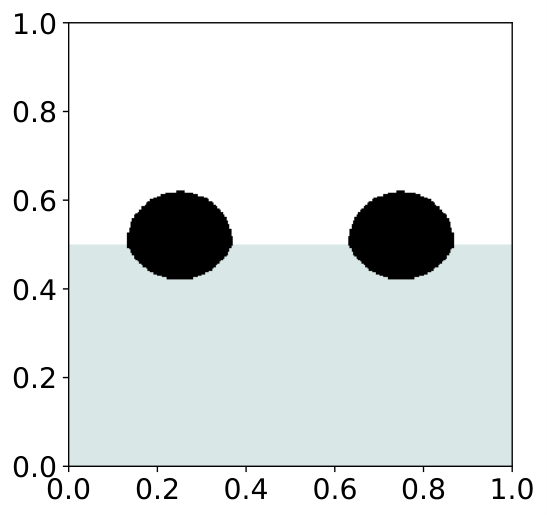
Refer to caption
Refer to caption
Refer to caption
Figure 4. Initialization (left), ground truth σ⁡(𝛀⋆)\sigma(\mathbf{\Omega}^{\star}) (center) and reconstruction σ⁡(𝛀rec)\sigma(\mathbf{\Omega}^{\text{rec}}) using 1111 boundary currents with 0%0\% noise and E⁡(𝛀rec)=5.72%E(\mathbf{\Omega}^{\text{rec}})=5.72\% reconstruction error (right). The conductivity values are σ0,0=1\sigma_{0,0}=1 (white), σ1,0=3\sigma_{1,0}=3 (light gray), σ2,0=15\sigma_{2,0}=15 (black).
Refer to caption
Refer to caption
Refer to caption
Refer to caption
Figure 5. Ground truth σ⁡(𝛀⋆)\sigma(\mathbf{\Omega}^{\star}) (top left), reconstructions σ⁡(𝛀rec)\sigma(\mathbf{\Omega}^{\text{rec}}) using 1111 boundary currents with 0%0\% noise and E⁡(𝛀rec)=5.72%E(\mathbf{\Omega}^{\text{rec}})=5.72\% error (top right), with 1.02%1.02\% noise and E⁡(𝛀rec)=6.19%E(\mathbf{\Omega}^{\text{rec}})=6.19\% error (bottom left), with 2.03%2.03\% noise and E⁡(𝛀rec)=6.81%E(\mathbf{\Omega}^{\text{rec}})=6.81\% error (bottom right). The conductivity values are σ0,0=1\sigma_{0,0}=1 (white), σ1,0=3\sigma_{1,0}=3 (light gray), σ2,0=15\sigma_{2,0}=15 (black). The initialization is shown in Figure 4(left).

Acknowledgments.

The author would like to thank Prof. James A. Sethian for the discussion about the tracking of interfaces in multiphase problems and the inspiration to work on this topic.

Funding

The author gratefully acknowledges the support of the Brazilian National Council for Scientific and Technological Development (Conselho Nacional de Desenvolvimento Científico e Tecnológico - CNPq) through the process: 408175/2018-4 “Otimização de forma não suave e controle de problemas de fronteira livre”, and through the program “Bolsa de Produtividade em Pesquisa - PQ 2018”, process: 304258/2018-0.

References

  • [1] G. Alessandrini, M. V. de Hoop, R. Gaburro, and E. Sincich. EIT in a layered anisotropic medium. Inverse Probl. Imaging, 12(3):667–676, 2018.
  • [2] G. Allaire, C. Dapogny, G. Delgado, and G. Michailidis. Multi-phase structural optimization via a level set method. ESAIM Control Optim. Calc. Var., 20(2):576–611, 2014.
  • [3] J. W. Barrett, H. Garcke, and R. Nürnberg. On sharp interface limits of Allen-Cahn/Cahn-Hilliard variational inequalities. Discrete Contin. Dyn. Syst. Ser. S, 1(1):1–14, 2008.
  • [4] T. K. Bera. Applications of electrical impedance tomography (EIT): A short review. IOP Conference Series: Materials Science and Engineering, 331:012004, mar 2018.
  • [5] E. Beretta, E. Francini, and S. Vessella. Differentiability of the Dirichlet to Neumann map under movements of polygonal inclusions with an application to shape optimization. SIAM J. Math. Anal., 49(2):756–776, 2017.
  • [6] E. Beretta, S. Micheletti, S. Perotto, and M. Santacesaria. Reconstruction of a piecewise constant conductivity on a polygonal partition via shape optimization in EIT. J. Comput. Phys., 353:264–280, 2018.
  • [7] L. Borcea. Electrical impedance tomography. Inverse Problems, 18(6):R99–R136, 2002.
  • [8] L. Bronsard, H. Garcke, and B. Stoth. A multi-phase Mullins-Sekerka system: matched asymptotic expansions and an implicit time discretisation for the geometric evolution problem. Proc. Roy. Soc. Edinburgh Sect. A, 128(3):481–506, 1998.
  • [9] L. Bronsard and B. T. R. Wetton. A numerical method for tracking curve networks moving with curvature motion. J. Comput. Phys., 120(1):66–87, 1995.
  • [10] S. Chen, S. Gonella, W. Chen, and W. K. Liu. A level set approach for optimal design of smart energy harvesters. Comput. Methods Appl. Mech. Engrg., 199(37-40):2532–2543, 2010.
  • [11] M. Delfour, G. Payre, and J.-P. Zolésio. An optimal triangulation for second-order elliptic problems. Comput. Methods Appl. Mech. Engrg., 50(3):231–261, 1985.
  • [12] M. C. Delfour and J.-P. Zolésio. Shapes and geometries, volume 22 of Advances in Design and Control. Society for Industrial and Applied Mathematics (SIAM), Philadelphia, PA, second edition, 2011. Metrics, analysis, differential calculus, and optimization.
  • [13] H. Garcke, B. Nestler, and B. Stoth. A multiphase field concept: numerical simulations of moving phase boundaries and multiple junctions. SIAM J. Appl. Math., 60(1):295–315, 2000.
  • [14] F. Gibou, R. Fedkiw, and S. Osher. A review of level-set methods and some recent applications. Journal of Computational Physics, 353:82–109, Jan. 2018.
  • [15] M. Hintermüller and A. Laurain. Electrical impedance tomography: from topology to shape. Control Cybernet., 37(4):913–933, 2008.
  • [16] M. Hintermüller and A. Laurain. Multiphase image segmentation and modulation recovery based on shape and topological sensitivity. J. Math. Imaging Vision, 35(1):1–22, 2009.
  • [17] M. Hintermüller, A. Laurain, and A. A. Novotny. Second-order topological expansion for electrical impedance tomography. Adv. Comput. Math., 36(2):235–265, 2012.
  • [18] R. Hiptmair, A. Paganini, and S. Sargheini. Comparison of approximate shape gradients. BIT Numerical Mathematics, 55(2):459–485, Aug. 2014.
  • [19] J. Lamboley and M. Pierre. Structure of shape derivatives around irregular domains and applications. J. Convex Anal., 14(4):807–822, 2007.
  • [20] A. Laurain. Stability analysis of the reconstruction step of the voronoi implicit interface method. SIAM Journal on Numerical Analysis, 55(1):1–30, Jan. 2017.
  • [21] A. Laurain. Distributed and boundary expressions of first and second order shape derivatives in nonsmooth domains. Journal de Mathématiques Pures et Appliquées, 2019.
  • [22] A. Laurain and K. Sturm. Distributed shape derivative via averaged adjoint method and applications. ESAIM Math. Model. Numer. Anal., 50(4):1241–1267, 2016.
  • [23] H. Li and X.-C. Tai. Piecewise constant level set method for multiphase motion. Int. J. Numer. Anal. Model., 4(2):291–305, 2007.
  • [24] D. Liu, A. K. Khambampati, S. Kim, and K. Y. Kim. Multi-phase flow monitoring with electrical impedance tomography using level set based method. Nuclear Engineering and Design, 289:108 – 116, 2015.
  • [25] D. Liu, Y. Zhao, A. K. Khambampati, A. Seppänen, and J. Du. A parametric level set method for imaging multiphase conductivity using electrical impedance tomography. IEEE Transactions on Computational Imaging, 4(4):552–561, Dec 2018.
  • [26] A. Logg, K.-A. Mardal, and G. N. Wells, editors. Automated Solution of Differential Equations by the Finite Element Method, volume 84 of Lecture Notes in Computational Science and Engineering. Springer, 2012.
  • [27] Y. Mei and X. Wang. A level set method for structural topology optimization with multi-constraints and multi-materials. Acta Mech. Sin. Engl. Ser., 20(5):507–518, 2004.
  • [28] B. Merriman, J. K. Bence, and S. J. Osher. Motion of multiple functions: a level set approach. J. Comput. Phys., 112(2):334–363, 1994.
  • [29] W. Noh and P. Woodward. Slic (simple line interface calculation). In A. van de Vooren and P. Zandbergen, editors, Proceedings of the Fifth International Conference on Numerical Methods in Fluid Dynamics June 28 - July 2, 1976 Twente University, Enschede, volume 59 of Lecture Notes in Physics, pages 330–340. Springer Berlin Heidelberg, 1976.
  • [30] S. Osher and J. A. Sethian. Fronts propagating with curvature-dependent speed: algorithms based on Hamilton-Jacobi formulations. J. Comput. Phys., 79(1):12–49, 1988.
  • [31] L. Qi. Transposes, L-eigenvalues and invariants of third order tensors, 2017.
  • [32] R. I. Saye and J. A. Sethian. The Voronoi implicit interface method for computing multiphase physics. Proc. Natl. Acad. Sci. USA, 108(49):19498–19503, 2011.
  • [33] R. I. Saye and J. A. Sethian. Multiscale modeling of membrane rearrangement, drainage, and rupture in evolving foams. Science, 340(6133):720–724, 2013.
  • [34] J. A. Sethian. Level set methods and fast marching methods, volume 3 of Cambridge Monographs on Applied and Computational Mathematics. Cambridge University Press, Cambridge, second edition, 1999. Evolving interfaces in computational geometry, fluid mechanics, computer vision, and materials science.
  • [35] K. A. Smith, F. J. Solis, and D. L. Chopp. A projection method for motion of triple junctions by levels sets. Interfaces Free Bound., 4(3):263–276, 2002.
  • [36] J. Sokołowski and J.-P. Zolésio. Introduction to shape optimization, volume 16 of Springer Series in Computational Mathematics. Springer-Verlag, Berlin, 1992. Shape sensitivity analysis.
  • [37] K. Sturm. Minimax Lagrangian approach to the differentiability of nonlinear PDE constrained shape functions without saddle point assumption. SICON, 53(4):2017–2039, 2015.
  • [38] K. Sturm. A structure theorem for shape functions defined on submanifolds. Interfaces Free Bound., 18(4):523–543, 2016.
  • [39] X.-C. Tai and T. F. Chan. A survey on multiple level set methods with applications for identifying piecewise constant functions. Int. J. Numer. Anal. Model., 1(1):25–47, 2004.
  • [40] R. Tavakoli and S. M. Mohseni. Alternating active-phase algorithm for multimaterial topology optimization problems: a 115-line MATLAB implementation. Struct. Multidiscip. Optim., 49(4):621–642, 2014.
  • [41] L. A. Vese and T. F. Chan. A multiphase level set framework for image segmentation using the mumford and shah model. International Journal of Computer Vision, 50(3):271–293, Dec 2002.
  • [42] P. Vogiatzis, S. Chen, X. Wang, T. Li, and L. Wang. Topology optimization of multi-material negative Poisson’s ratio metamaterials using a reconciled level set method. Comput.-Aided Des., 83:15–32, 2017.
  • [43] M. Y. Wang and X. Wang. “Color” level sets: a multi-phase method for structural topology optimization with multiple materials. Comput. Methods Appl. Mech. Engrg., 193(6-8):469–496, 2004.
  • [44] Y. Wang, Z. Luo, Z. Kang, and N. Zhang. A multi-material level set-based topology and shape optimization method. Comput. Methods Appl. Mech. Engrg., 283:1570–1586, 2015.
  • [45] X. Zhang, J.-S. Chen, and S. Osher. A multiple level set method for modeling grain boundary evolution of polycrystalline materials. Interaction and multiscale mechanics, 1(2):191–209, 2008.
  • [46] H.-K. Zhao, T. Chan, B. Merriman, and S. Osher. A variational level set approach to multiphase motion. J. Comput. Phys., 127(1):179–195, 1996.
  • [47] J.-P. Zolésio. Identification de domaines par déformations. Thèse de doctorat d’état, Université de Nice, France, 1979.
  • [48] W. Zuo and K. Saitou. Multi-material topology optimization using ordered SIMP interpolation. Struct. Multidiscip. Optim., 55(2):477–491, 2017.