Lattice QCD Determination of the Bjorken- Dependence of Parton Distribution Functions at Next-to-next-to-leading Order
Abstract
We report the first lattice QCD calculation of pion valence quark distribution with next-to-next-to-leading order perturbative matching correction, which is done using two fine lattices with spacings fm and fm and valence pion mass MeV, at boost momentum as large as GeV. As a crucial step to control the systematics, we renormalize the pion valence quasi distribution in the recently proposed hybrid scheme, which features a Wilson-line mass subtraction at large distances in coordinate space, and develop a procedure to match it to the scheme. We demonstrate that the renormalization and the perturbative matching in Bjorken- space yield a reliable determination of the valence quark distribution for with 5–20% uncertainties.
Understanding the hadron inner structure remains one of the top fundamental questions in nuclear and particle physics. As the lightest hadrons in nature, pions are the Nambu-Goldstone bosons of quantum chromodynamics (QCD), and their quark and gluon structures can help understand the origins of hadron mass and dynamical chiral symmetry breaking. The parton distribution functions (PDFs), which describe 1D momentum densities of quarks and gluons in a hadron, are the simplest and most important quantities that have been extensively studied from global high-energy scattering experiments and will be probed at unprecedented precision at the future Electron-Ion Collider Accardi et al. 2016; Abdul Khalek et al. 2021. Besides the experimental efforts, the first-principles calculations of PDFs using lattice QCD are also expected to provide useful predictions.
Computation of the PDFs on a Euclidean lattice has been extremely difficult because they are defined from light-cone correlations with real-time dependence in Minkowski space. For a long time, only the lowest moments of the PDFs were calculable as they are matrix elements of local gauge-invariant operators. For reviews see Refs. Lin et al. 2018; Constantinou et al. 2021. Less than a decade ago, a breakthrough was made by large-momentum effective theory (LaMET) Ji 2013; Ji 2014; Ji et al. 2021a, which starts from a Euclidean “quasi-PDF” (qPDF) in a boosted hadron and obtains the PDF through a large-momentum expansion and perturbative matching of the qPDF in Bjorken- (longitudinal momentum fraction) space. Over the years, LaMET has led to much progress in the calculation of PDFs and other parton physics Ji et al. 2021a; Constantinou et al. 2021, which reinvigorated the field as other proposals Liu and Dong 1994; Detmold and Lin 2006; Braun and Müller 2008; Chambers et al. 2017; Radyushkin 2017; Ma and Qiu 2018a are also being studied and implemented.
Despite substantial progress, lattice calculation of the PDF -dependence has yet to achieve essential control of the systematic uncertainties Alexandrou et al. 2019. In the LaMET approach, lattice renormalization is one of the most important sources of error. The nonlocal quark bilinear operator , where is a Dirac matrix and , which defines the qPDF, suffers from a linear power divergence in the Wilson line that must be subtracted before taking the continuum limit. The most popular methods so far are the regularization independent momentum subtraction scheme Constantinou and Panagopoulos 2017; Stewart and Zhao 2018; Alexandrou et al. 2017; Chen et al. 2018 and other ratio schemes Orginos et al. 2017; Braun et al. 2019; Li et al. 2021; Fan et al. 2020, which use the matrix element of in an off-shell quark Constantinou and Panagopoulos 2017; Stewart and Zhao 2018; Alexandrou et al. 2017; Chen et al. 2018, a static/boosted hadron Orginos et al. 2017; Fan et al. 2020 or the vacuum state Braun et al. 2019; Li et al. 2021 as the renormalization factor. At small the matrix elements in these schemes satisfy a factorization relation to the light-cone correlation Ji et al. 2017; Radyushkin 2018; Ma and Qiu 2018a; Izubuchi et al. 2018. However, at large they introduce nonperturbative effects Gao et al. 2020 that propagate to the qPDF via Fourier transform (FT) of the matrix elements, which contaminates the LaMET matching in -space. To overcome this limitation, the hybrid scheme Ji et al. 2021b was proposed to subtract the linear divergence at large and match the result to the scheme, thus preserving the LaMET matching after FT. To date, the hybrid scheme has not been used in calculating the PDFs, except for a recent work on meson distribution amplitudes Hua et al. 2021. Apart from renormalization, the accuracy of perturbative matching also controls the precision of the calculation. In all the existing lattice calculations, the matching was done at only next-to-leading order (NLO), and it is not until recently that the next-to-next-to-leading order (NNLO) matching was derived for the non-singlet quark qPDF in the scheme Chen et al. 2021; Li et al. 2021.
In this Letter we present a state-of-the-art calculation of pion valence quark PDF using high-statistics, superfine-spacing, and large-momentum lattice data Gao et al. 2020, with an adapted hybrid-scheme renormalization and the first-time implementation of NNLO matching. The pion valence PDF has been extracted from global fits Gluck et al. 1992; Novikov et al. 2020; Barry et al. 2021; Aicher et al. 2010 and studied in lattice QCD Zhang et al. 2019; Sufian et al. 2019; Izubuchi et al. 2019; Joó et al. 2019; Sufian et al. 2020; Lin et al. 2021; Gao et al. 2020; Gao et al. 2021, with both at NLO accuracy. In this work, we subtract the linear divergence in with sub-percent precision, and develop a procedure to match the lattice subtraction scheme to , a crucial step in the hybrid scheme to reduce the power corrections Ji et al. 2021b. We derive the NNLO hybrid-scheme matching and apply it to the qPDF, showing good perturbative convergence and reduced scale-variation uncertainty compared to NLO matching. Finally, we demonstrate that our analysis yields a reliable determination of the PDF for with 5–20% uncertainties.
Our lattice data was produced using gauge ensembles in 2+1 flavor QCD generated by the HotQCD collaboration Bazavov et al. 2014 with Highly Improved Staggered Quarks Follana et al. 2007, including two lattice spacings and fm, and volumes and , respectively. We use tadpole-improved clover Wilson valence fermions on the hypercubic (HYP) smeared Hasenfratz and Knechtli 2001 gauge background, with a valence pion mass MeV. Furthermore, the Wilson line in is constructed from HYP-smeared gauge links. We use pion momenta with , resulting in as large as GeV.
The qPDF is defined in a boosted pion state with four-momentum :
| (1) |
where , and is the scale. The operator can be renormalized under lattice regularization as Ji et al. 2018; Ishikawa et al. 2017; Green et al. 2018
| (2) |
where “” and “” denote bare and renormalized quantities. The factor includes all the logarithmic ultraviolet (UV) divergences which are independent of , while the Wilson-line mass correction includes the linear UV divergence and can be expressed as
| (3) |
where is a series in the strong coupling , and is an constant originating from the renormalon ambiguity in Bauer et al. 2012.
The hybrid scheme is implemented as follows: For with , we form the ratio to cancel the UV divergences and the cutoff effects from Orginos et al. 2017; at we subtract and determine by imposing a continuity condition of the renormalized matrix elements at . There are different ways to calculate Ji et al. 2021b; Zhang et al. 2017; Green et al. 2018; Green et al. 2020; Alexandrou et al. 2021; Huo et al. 2021. We determine from the combination of the static quark-antiquark potential, Bazavov et al. 2014; Bazavov et al. 2018a, and the free energy of a static quark at non-zero temperature Bazavov et al. 2016; Bazavov et al. 2018b; Petreczky et al. 2021, with the following normalization scheme,
| (4) |
where fm is the Sommer scale for 2+1 flavor QCD Bazavov et al. 2014, and the constant 0.95 defines the scheme. The linear divergence does not depend on the scheme, while does. The results are and for and fm, respectively.
Since is scheme dependent, a factor of with is needed to match the lattice scheme to , otherwise the LaMET expansion of the qPDF will include a power correction Ji et al. 2021b, which slows down convergence to the PDF as grows. It was proposed that can be obtained by comparing the subtracted matrix elements of Huo et al. 2021 or Green et al. 2020 with their operator product expansion (OPE), whose accuracy requires fm Ji et al. 2021b. But due to discretization effects, the window of that can be used is actually narrow.
Our new procedure for the hybrid scheme is distinct by the determination of . In order to use larger , we construct the following ratio and compare it to a form motivated by the OPE of ,
| (5) |
where , and the parameter . The Wilson coefficient is known to NNLO Izubuchi et al. 2018; Chen et al. 2021; Li et al. 2021, and and originate from the leading UV and infrared renormalons in Braun et al. 2019. According to Eq. (2), the l.h.s. of Eq. (5) must have a continuum limit if includes all the linear divergences, which is renormalization group (RG) invariant. We choose fm and find agreement between the fm and fm ratios at sub-percent level up to fm (see App. A). Then we extrapolate the lattice ratios to the continuum with -dependence Gao et al. 2020, and fit the result to the r.h.s of Eq. (5). For fm, we obtain decent plateaus and values for both and with the NNLO . By definition cancels the lattice scheme dependence of , as changing the scheme only shifts by a constant, but will inherit the ambiguity in the scheme. Since is at fixed order, both and depend on , which we vary to estimate the related uncertainty in the final result. At GeV, GeV and GeV2, so the power correction is not negligible. Therefore, we modify the hybrid scheme by correcting the term in at short as
| (6) |
where , and normalizes to one at . Since is at fixed order, depends on despite the fact that it should be RG invariant. Such a renormalization is performed through bootstrap loops so that the correlation between different and is taken care of.
The hybrid-scheme matrix elements are shown in Fig. 1. At small , is dominated by the leading-twist contribution. At large , the spacelike correlator for pion valence quarks will exhibit an exponential decay where is an effective mass related to the system Burkardt et al. 1995. When plotted as a function of , should scale in at small , with slight violation due to QCD evolution. Its exponential decay will emerge at a larger with greater and with decay rate . In the limit, the exponential decay vanishes at finite (), and only the leading-twist contribution remains, which almost scales in and features a power-law decay at large that corresponds to small- PDF Ji et al. 2021b. This picture is consistent with Fig. 1.

The next step is a FT. We truncate the matrix elements at or where , and extrapolate to to remove the unphysical oscillations from a truncated FT Ji et al. 2021b. The extrapolation form is , where , and are the parameters. Since is independent of , by fitting to the matrix elements we find that it is around GeV, which is not far from the phenomenological estimate of 0.2–0.5 GeV in HQET Beneke and Braun 1994. Therefore, we impose GeV, as well as and , to ensure a convergent FT on each bootstrap sample. Since the FT converges fast with the exponential decay, the extrapolation mainly affects the small- region apart from removing the unphysical oscillations. To verify this we vary , which turns out to have little impact, and use different bounds and extrapolation forms, which lead to consistent qPDFs down to . (See App. B).
Then, we match the qPDF to the PDF through LaMET Xiong et al. 2014; Ma and Qiu 2018b; Izubuchi et al. 2018; Ji et al. 2021b:
| (7) |
where , fm, and the power corrections are controlled by the parton and spectator momenta and Ji et al. 2021b. Here is the inverse of the hybrid-scheme matching coefficient , which we derive at NNLO Zhao et al. by conversion from the result Chen et al. 2021; Li et al. 2021. Based on Eq. (Lattice QCD Determination of the Bjorken- Dependence of Parton Distribution Functions at Next-to-next-to-leading Order), we can directly calculate the PDF with -controlled power corrections for .

In Fig. 2 we show the results of perturbative matching. The matching drives the qPDF to smaller and reduces the statistical errors at moderate , because matching effectively relates the qPDF from finite to infinity, and the qPDF evolves to smaller as increases. The NNLO correction is generally smaller than the NLO correction, which indicates good perturbative convergence, a crucial criterion for precision calculation. Besides, by varying and evolving the matched results to the same , we find that the scale-variation uncertainty is reduced at NNLO, which is further evidence of improved precision. The matching correction diverges as , implying that resummation of small- logarithms is needed. A resummation is also necessary as Gao et al. 2021, but these resummations are not needed for moderate .
We compare the PDFs obtained at different with NNLO matching in Fig. 3. At moderate , the -dependence is remarkably reduced, and the results appear to converge for GeV, which strongly indicates the effectiveness of LaMET matching. At , each PDF curve has a small non-vanishing tail due to the power corrections in Eq. (Lattice QCD Determination of the Bjorken- Dependence of Parton Distribution Functions at Next-to-next-to-leading Order), but they decrease with larger (see also App. C.3). To estimate the size of the power corrections, we fit the PDFs obtained at fm, GeV and fm, GeV to the ansatz for each fixed , where we ignore the -dependence as it has been found that the matrix elements have effects that are less than 1% Gao et al. 2020. Since this fit is mainly affected by the data sets at lower with smaller statistical errors, which have larger power corrections, we use the result at GeV instead of the fitted as our final prediction. The power correction at GeV is estimated to be for . It is surprising that the results are insensitive to for as small as , nor do they show dependence on the extrapolation form in the FT as we have checked. This can be explained by that, under matching, the qPDF contributes to the PDF at larger which has less dependence on or the extrapolation. Nevertheless, it must be pointed out that the smallness here is only relative, as still diverges as .

Our final prediction for the pion valence quark PDF (BNL-ANL21) is shown in Fig. 4, which is obtained from the qPDF at fm, fm, fm, GeV and GeV with exponential extrapolation and NNLO matching. The red band represents the statistical error, and the light purple band includes the error from scale variations, which is obtained by repeating the same analysis for GeV and GeV and evolving the PDFs to GeV with the NLO DGLAP kernel. Since the hybrid-scheme parameter depends on , the small scale variation in the final result shows that the renormalization uncertainty is well under control. We require that the matching correction at GeV be smaller than 5%, which propagates geometrically to at NLO and at NNLO, thus excluding and . A list of the above uncertainties at selected is shown in Table 1. See also App. D. We neglect the FT uncertainty as it is extremely small. As for dependence, our associated calculation of the second PDF moment at MeV Gao 2021 shows consistency within 5% statistical uncertainty, which will be validated by a direct comparison in the future. Previous studies Lin and Zhang 2019; Liu and Chen 2021 also suggest that the finite volume correction is less than 1% for our lattice setup. At last, by limiting the estimated power corrections to be less than 10%, we determine the PDF at with 5–20% uncertainties. Our result is in great agreement with the recent global fits by xFitter Novikov et al. 2020 and JAM21nlo Barry et al. 2021 for , but deviates from the earlier GRVPI1 Gluck et al. 1992 and ASV Aicher et al. 2010 fits. When compared to a previous analysis of the same lattice data (BNL20) Gao et al. 2020, which used a short-distance factorization of the matrix elements at NLO, and a parameterization of the PDF, our new result has shifted central values and considerably reduced uncertainties at moderate , but still agrees within errors. With finite and statistics, lattice QCD can only make predictions for . The PDF parameterization correlates the information at all , so the larger uncertainties at moderate in BNL20 could be propagated from the uncontrolled errors in the end-point regions. Besides, there is no practical estimate of the model uncertainty in the parameterization. Therefore, the LaMET calculation for is more reliable as it does the power expansion and matching directly in -space.

| Statistical | Scale | Power corrections | |||
|---|---|---|---|---|---|
| 0.03 | 0.10 | 0.04 | |||
| 0.40 | 0.07 | 0.04 | |||
| 0.80 | 0.15 | 0.03 | 0.10 |
In summary, we have performed a state-of-the-art lattice QCD calculation of the -dependence of pion valence quark PDF, where we developed a procedure to renormalize the qPDF in the hybrid scheme and match it to the PDF at NNLO. The final results show reduced perturbation theory uncertainty and converge at moderate with pion momenta greater than GeV, which allows us to reliably estimate the systematic errors. This calculation can be improved with physical pion mass, continuum extrapolation, and higher statistics for the matrix elements at long distances and at larger boost momenta.
Our renormalization procedure can also be incorporated into the lattice calculations of gluon PDFs, distribution amplitudes, generalized parton distributions and transverse momentum distributions. With the systematics under control, we can expect lattice QCD to provide reliable predictions for these quantities in the future.
Acknowledgements.
We thank Vladimir Braun, Xiangdong Ji, Nikhil Karthik, Yizhuang Liu, Antonio Pineda, Yushan Su and Jianhui Zhang for valuable communications. This material is based upon work supported by: (i) The U.S. Department of Energy, Office of Science, Office of Nuclear Physics through Contract No. DE-SC0012704 and No. DE-AC02-06CH11357; (ii) The U.S. Department of Energy, Office of Science, Office of Nuclear Physics and Office of Advanced Scientific Computing Research within the framework of Scientific Discovery through Advance Computing (SciDAC) award Computing the Properties of Matter with Leadership Computing Resources; (iii) The U.S. Department of Energy, Office of Science, Office of Nuclear Physics, within the framework of the TMD Topical Collaboration. (iv) XG is partially supported by the NSFC under the grant number 11775096 and the Guangdong Major Project of Basic and Applied Basic Research No. 2020B0301030008. (v) SS is supported by the National Science Foundation under CAREER Award PHY-1847893 and by the RHIC Physics Fellow Program of the RIKEN BNL Research Center.. (vi) This research used awards of computer time provided by the INCITE and ALCC programs at Oak Ridge Leadership Computing Facility, a DOE Office of Science User Facility operated under Contract No. DE-AC05-00OR22725. (vii) Computations for this work were carried out in part on facilities of the USQCD Collaboration, which are funded by the Office of Science of the U.S. Department of Energy. viii) YZ is partially supported by an LDRD initiative at Argonne National Laboratory under Project No. 2020-0020.Appendix A Hybrid scheme renormalization
A.1 Definition of scheme
As has been described in the main text, the hybrid scheme renormalization includes two parts:
- •
For , we form the ratio of bare matrix elements Orginos et al. 2017,
(8) which has a well-defined continuum limit and is renormalization group (RG) invariant.
- •
For , the renormalized matrix element is
(9) which is equal to the ratio in Eq. (8) at . To determine we use the additive renormalization constant, , which is obtained in Ref. Bazavov et al. 2018b from the analysis of the free energy of a static quark, , at non-zero temperature with the normalization condition in Eq. (4). Recently has been calculated using one step of HYP smearing Petreczky et al. 2021, and it was found that HYP smearing does not affect the temperature dependence of , but only shifts it by an additive constant. Therefore, we have with superscripts 0 and 1 referring to the number of HYP smearing steps in the bare free energy of the static quark. Using the lattice results for and obtained on lattices and temperatures corresponding to fm and fm (where cutoff effects can be neglected), as well as the values of from Table X of Ref. Bazavov et al. 2018b for ( fm) and ( fm), we obtain . The results are and .
First of all, to test how well the subtraction of can remove the linear divergences in , we construct the ratio in Eq. (5),
| (10) |
where fm for both lattice spacings. According to Eq. (2), the renormalization factor cancels out in the ratio. Therefore, if includes all the linear divergences, then should have a well-defined continuum limit.

Our lattice results for the above ratio with fm is shown in Fig. 5. As one can see, the differences between the ratios at fm and fm are at sub-percent level, which clearly shows that the linear divergences have been sufficiently subtracted by . Therefore, the ratio in Eq. (10) has a continuum limit
| (11) |
which is RG invariant.
Our next step is to match the lattice subtraction scheme to . When , the matrix element has an OPE that goes as
| (12) |
where is the renormalon ambiguity from the Wilson line self-energy renormalization Braun et al. 2019, is a twist-four operator (for example, or ), and are perturbative coefficient functions, and “” denotes contributions at higher twists. Since , is the only Wilson coefficient that contributes at leading-twist. The leading-twist contribution is proportional to which is trivially one due to vector current conservation. Since is multiplicatively renormalizable, both and must satisfy RG equations with the same anomalous dimension, which is known to next-to-next-to-next-to-leading order (N3LO) Braun et al. 2020. Due to the ambiguity in summing the perturbative series in , there are IR renormalons in the leading-twist contribution that should be cancelled by those from higher-twist condensates, along with the UV renormalon to be cancelled by Braun et al. 2019; Beneke and Braun 1994. Both the UV and IR renormalon contributions cannot be well defined unless one specifies how to sum the perturbative series in to all orders, which, however, is unknown as has been calculated to only NNLO so far Li et al. 2021.
Note that is analogous to the mass renormalization in heavy-quark effective theory (HQET) Beneke and Braun 1994, which is of UV origin and cannot be attributed to any short-distance condensate. Instead, it appears as a residual mass term in the HQET Lagrangian and exists in at all , i.e.,
| (13) |
where at short distance reduces to the OPE series in the brackets of Eq. (A.1).
The renormalons have been studied extensively for the Polyakov loop and plaquette in lattice QCD Bauer et al. 2012; Bali et al. 2013; Bali et al. 2014a; Bali et al. 2014b; Bali et al. 2014c. In lattice perturbation theory, one has to compute the perturbative series to very high orders of in order to see the renormalon effects. Nevertheless, in the scheme, the OPE with Wilson coefficient at a few loop orders and the condensate term, turns out to be successful in describing the static potential at short distance up to fm Pineda 2003. One explanation is that in the scheme is larger than that in lattice perturbation theory, so the renormalon effect which is of with becomes significant at lower orders. This situation is similar to the OPE in QCD sum rules Shifman et al. 1979a; Shifman et al. 1979b; Novikov et al. 1984; Novikov et al. 1985; David 1986, which works well in phenomenology. The reason behind such success is probably due to a proper choice of the renormalization scale so that is small enough for the perturbative series to converge, while the -dependent effects in the condensate remain insignificant as they should be of the same magnitude of highest order in the truncated perturbative series Novikov et al. 1985; David 1986.
Therefore, we approximate Eq. (A.1) as
| (14) |
where “FO” stands for fixed order, is a parameter of , and we ignore the higher power corrections by working at not too large . The dependence of the parameters and is understandable because this approximation is valid for a small window of , and they also depend on the perturbative orders in if the latter does not converge fast. Note that the although the model in Eq. (14) is not guaranteed to satisfy the RG equation for , we argue that within the range of where it can describe the physical results, the -dependence in the power correction term, which is already suppressed, is weak and can be ignored.
Based on the above approximation, we fit our lattice results of the ratio in Eq. (10) to the following ansatz,
| (15) |
where the mass shift
| (16) |
cancels the lattice scheme dependence of in Eq. (3) and introduces the renormalon ambiguity of the scheme. Effectively, matches the hybrid-scheme matrix elements at to the ratio of as
| (17) |
Moreover, since the ansatz in Eq. (15) can describe the short-distance matrix elements well, we can correct the term in at as
| (18) |
which is equivalent to replacing by the perturbative , as in Eq. (Lattice QCD Determination of the Bjorken- Dependence of Parton Distribution Functions at Next-to-next-to-leading Order). Eventually, the continuum limit of the matched matrix element in Eq. (Lattice QCD Determination of the Bjorken- Dependence of Parton Distribution Functions at Next-to-next-to-leading Order) is
| (19) |
which is different from through a perturbative matching for all as long as . Therefore, the qPDF defined as FT of is still factorizable.
Note that introduces the ambiguity to the matched matrix elements. Nevertheless, we argue that at NNLO is different from a particular summation prescription by contributions, which cannot be smaller than the ambiguity in as the latter reflects the uncertainty in summing divergent perturbative series at sufficiently high orders. Therefore, we can attribute the renormalon ambiguity in to higher loop-order effects, and estimate the latter by varying by a factor of and . The range of we vary from cannot be too large. If is too small, then becomes too large; if is too large, then we need to resum the large in . In both cases the perturbative series converges slowly. In our analysis, we scan within GeV for and GeV for to study the scale dependence and uncertainty from renormalon ambiguity.
A.2 Fitting of and
Currently, the Wilson coefficient is known to NNLO Chen et al. 2021; Li et al. 2021 and its anomalous dimension has been calculated at three-loop order Braun et al. 2020,
| (20) |
where , , and ,. The factor in the last square bracket is a simple guess by assuming that the constant part of the perturbative correction grows as a geometric series in the order of .
We also consider the RG improved (RGI) Wilson coefficient Gao et al. 2021
| (21) | ||||
where is the anomalous dimension of the operator , and . In this way, we can first factor out the evolution factor in Eq. (14) as it must be satisfied by the full matrix element , and therefore construct the ratio in an explicitly -independent way.
We compare and at NLO, NNLO and N3LO at GeV in Fig. 6. The strong coupling constants at each perturbative order are defined by the corresponding with one-, two- and three- loop functions and , which are fixed by matching to . The latter is obtained from MeV with five-loop -function and , as has been calculated using the same lattice ensembles Petreczky and Weber 2020. As one can see, at fm the RGI Wilson coefficients start to deviate significantly from the fixed-order ones, which is mainly due to the large value of as in RGI Wilson coefficients as we evolve from to . This indicates that at fm, the scale uncertainty in the perturbative series is significant due to the enhancement of non-perturbative effects, and to use OPE we should work at very short distances ( fm). However, there will not be enough room for varying to satisfy so that discretization effects are suppressed. Therefore, in our analysis we loosen our requirement for very small by only using the ansatz in Eq. (15) and not considering the RGI Wilson coefficients.
In Fig. 7a, we plot an effective mass which is defined as
| (22) |
where GeV. If the twist-four condensate is negligible, then we should expect a plateau in , but Fig. 7a shows that it has an almost constant nonzero slope at from fm up to fm. In Fig. 7b we plot its slope
| (23) |
which is consistent with being constant for a wide range of . This suggests that there is considerable quadratic -dependence from the twist-four condensate, as inclued in the ansatz in Eq. (15).

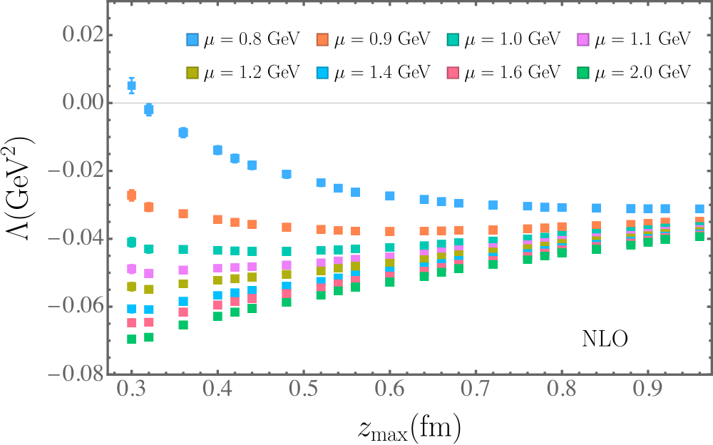

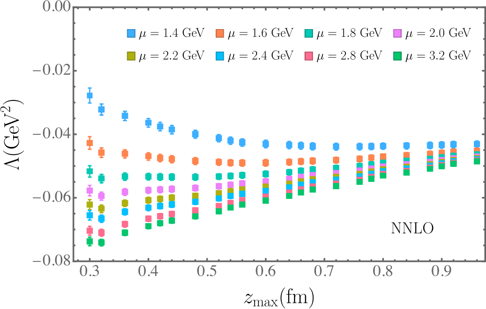
Our results for and fitted from for with fm are shown in Fig. 8. As one can see, the two parameters remain constant in up to around fm within a small window of , which is different with the NLO and NNLO Wilson coefficients. At larger , the higher-twist and effects become significant, which can no longer be described by the simple ansatz in Eq. (15). In this work, we use at fm fm to fit the parameters at all as input for the hybrid scheme renormalization and matching. To estimate the uncertainty from the choice of , we will match the qPDFs obtained at different to the corresponding PDFs, and then evolve the final results to GeV for comparison.
Appendix B Fourier transform (FT)
The qPDF is defined as the FT of or ,
| (24) |
Since is perturbatively matched from the scheme, the factorization formula should still be valid for the corresponding qPDF Ji et al. 2021b. Therefore, we should integrate over all in the FT to obtain the -dependence of the qPDF. However, due to finite lattice size effects, worsening signal-to-noise ratio and other systematics at large , we have to truncate at and extrapolate to to complete the FT. As a result, the small- () region is the most sensitive to the extrapolation model, and the corresponding systematic uncertainty cannot be well controlled. On the other hand, the reliability of the region depends on the premises that the is small at and exhibits an exponential decay when is large enough. The first condition is easy to understand as a truncated FT will lead to an unphysical oscillation in the -space with amplitude proportional to , while the exponential decay guarantees that the FT converges fast and the qPDF at has very little dependence on the specific model used in the extrapolation.
In this section, we first derive that the equal-time correlator in a hadron state does exhibit an exponential decay at large distances, then we demonstrate that including this constraint in the extrapolation will lead to a reliable FT in the moderate-to-large region. Finally, we perform the extrapolated FT on our lattice results.
B.1 Matrix elements at large
To begin with, let us consider a current-current correlation in the vacuum, , where and . If we ignore the existence of zero modes and only consider gapped vacuum excitations, then
| (25) |
where is the overlap between the operator and intermediate sate . Here is the mass of the intermediate state particle, and is the modified Bessel function of the second kind. Then, since
| (26) |
The correlation function should, therefore, be dominated by the exponential decay of the lowest-lying state that overlaps with .
When the external state is a static hadron, it has also been shown that the spacelike correlations exhibit an exponential decay at large distance Burkardt et al. 1995.
We are interested in equal-time quark bilinear correlators in a boosted hadron state, which can be expressed in terms of the product of two “heavy-light” currents Ji et al. 2018; Green et al. 2018, where the “heavy quark” is an auxiliary field defined along the direction, similar to that in HQET.
Let us choose the external state to be a pion. According to Lorentz covariance, we can decompose the correlation as
| (27) |
where the scalar functions are analytic functions of and . We can select the index such that . For example, we can choose when or when . The HQET corresponds to the timelike case, as
| (28) |
where is the effective heavy-quark field moving with velocity and related to the QCD heavy quark by the projection
| (29) |
The lowest intermediate state is a heavy-light meson with mass and momentum , where is the heavy quark pole mass, and can be interpreted as the mass of the constituent light quark or binding energy. Both and have renormalon ambiguities which cancel between each other. In the limit, should be independent of the heavy quark mass, but can depend on the light quark mass.
The matrix element is given by the transition form factors Falk et al. 1990,
| (30) |
where the form factors and only depend on in HQET, and the projetion operator depends on the spin of the heavy-light meson ,
with being the polarization vector for vector mesons. Therefore,
| (33) | ||||
| (34) |
Then, the correlation function becomes
| (35) |
Note that when , constitutes a large phase, so the integrand is quickly oscillating and should be suppressed. To have a naive estimate, let us assume and are constant in , and the remaining integral is simply
| (36) |
where we first obtained the result for imaginary and then analytically continued back to the real axis.
Then, using Lorentz invariance and analyticity, we can obtain the result for , which corresponds to the equal-time correlator that we calculate in this work. At large separation, we have
| (37) |
which also exhibits an exponential behavior with decay constant . Moreover, the correlation also includes a phase which becomes in the case of the valence quark distribution. Another important takeaway is that is a Lorentz-invariant quantity and should be independent of the external momentum.
However, it must be pointed out that the conclusion in Eq. (37) is based on a rather crude approximation that and are constant in . In practice, the transition form factors could have a pole at the mass of a heavy-light meson created by the current or , which is different from for the intermediate state . As a result, the binding energy would also be different. If we take this into account in Eq. (B.1), then the result will exhibit a more complicated asymptotic behavior at large distance,
| (38) |
where the decay constant should vary among the different binding energies for the heavy-light mesons, which is similar to the observation in Ref. Burkardt et al. 1995, and is a function that can have both oscillating and non-oscillating dependence on . For large enough , the exponential decay should suppress the correlation and make it or its extremes decrease monotonically in magnitude.
Note that after we match the hybrid scheme matrix elements to , the renormalon ambiguity in the Wilson line mass, , is subtracted out, so the matched result should exhibit an asymptotic behavior that goes as at large . Therefore, the sign of becomes crucial in determining whether it is exponentially decaying or growing.
In QCD sum rule calculations, the result is GeV from phenomenology, while is expected to be GeV Beneke and Braun 1994, so GeV. Since the quarks have heavier-than-physical masses in our lattice calculation, one should expect a larger , so it is very likely that still remains positive. After all, this can be always put to test on the matrix elements since is a Lorentz-invariant quantity.
B.2 Extrapolation and FT
If is large enough for the correlation to reach the asymptotic region, then an extrapolation that encodes the exponential decay behavior we derived in App. B.1 should lead to reliable FT for moderate-to-large . To be more precise, there is a rigorous upper bound for the uncertainty of FT which decreases with .
To prove the above statement, let us consider extrapolation based on the general model
| (39) |
where , and with being the effective mass for the exponential decay. Motivated by QCD sum rule results, we expect GeV, which can be larger since we have used heavier-than-physical quark masses. Therefore, for GeV in the current work, we should have or higher.
Now let us compare two extrapolations and with different and . The difference between the two extrapolations,
| (40) |
should satisfy and . The difference in the FT with extrapolation is therefore
| (41) |
If we can approximate as a flat curve within one period of the oscillatory function , then the integral in that region vanishes. This condition can be satisfied if , which should be reached very quickly due to the exponential suppression at large . For each , there should be a minimal integer which satisfies , so that we can approximate as
| (42) |
Since and , there must be at least one extremum of for , so we have the inequality
| (43) |
According to our estimate of , at GeV, so
| (44) |
and should be sufficient to satisfy with . Therefore, in Eq. (B.2) we demonstrate that there is an upper bound for the model uncertainty in the FT with exponential extrapolation, which decreases in . The error is also proportional to which can be much smaller than that is already close to zero. If , , and , then we have
| (45) |
which is less than 0.15 at and around 15% of the central value of the qPDF as we obtain below. It is worth pointing out that our estimate of the upper bound in Eq. (B.2) can be highly overestimated, as has an oscillation from and which are out of pace with for , and could be much smaller than and at a sharp peak within .
Therefore, the FT with exponential extrapolation is under control for moderate and large . When is small enough, the model uncertainty from the extrapolation can be controlled to be much smaller than the other systematic uncertainties which are about in this work.
It is worth to compare with the extrapolation error when the correlation function decreases algebraically as , which corresponds to the generic model
| (46) |
Suppose we truncate at , then
| (47) |
The power is related to the small- behavior of the PDF. If we parameterize the PDF as , then with LO matching one can derive that Ji et al. 2021b, which is empirically. Therefore, it will take for the factor in Eq. (47) to decrease sufficiently to satisfy the condition . As a result, the uncertainty in the FT is of orders of magnitude larger than that of extrapolation with exponential decay.
To test our claim of controlled FT error with exponential decay, we choose a particular model
| (48) |
Suppose that the extrapolation is done at with , and the parameters and are fitted with errors and , then we analytically FT the extrapolated result to the -space, and calculate its error using
| (49) |
In Fig. 9, we plot the extrapolation error against . We have chosen different central values of the parameters and and fairly large uncertainties in them. The parameter cannot have a large negative value, otherwise it would make grow beyond .
In most of the scenarios considered, the error is for . As we shall see below, the actual extrapolation error is much smaller than this estimate and thus negligible when compared to the other systematic errors.
In the following, we perform the extrapolation with four different models. The extrapolation is carried out on each bootstrap sample by a minimal-square fit. For each , we truncate at the largest , , where the central value of remains positive, and choose to estimate the truncation error. The range of used to fit the parameters is where satisfies . The continuty condition between data and model was imposed in the middle point of the fit range, namely , which is listed in Table 2. The extrapolation models are:
| fm | fm | |
| N/A | ||
Exponential decay model,
or “model-exp”. The model for extrapolation is
| (50) |
We have tried to fit from the same range of for matrix elements with a similar form, , and found that is around GeV, about the same scale as the phenomenological estimate. For the matrix elements, we do not fix , but constrain it with a prior . To test the dependence on this prior condition, we have set GeV. Besides, we also impose and to ensure that the extrapolated result is positive and decreases in .
Power-law decay model,
or “model-pow”. The model is defined by setting in model-exp. As the limit of model-exp, model-pow can be used to give a coarse estimate of the significance of higher-twist effects, although its FT error is not well under control as we discussed above. We impose the conditions so that the fitted results decrease to zero as .
Two-parameter model with exponential decay,
or “model-2p-exp”. As we can see from Fig. 1, the matrix elements at do not show a clear exponential decay, although they can be fitted by the latter with due to the large errors. This may indicate that there is oscillation in . To incorporate such dependence, we ignore the higher-twist contributions and assume that the qPDF is parameterized as
| (51) |
By doing an inverse FT into the -space, the asymptotic form of at large reads,
| (52) |
Then we multiply with an exponential decay factor as our model for extrapolation,
| (53) |
Two-parameter model,
or “model-2p”. Again, we ignore the exponential decay and use as the extrapolation model, which can help us estimate the significance of higher-twist effects.


In Fig. 10 we compare the FT with different for extrapolation with model-exp and condition GeV. Except for very small , the results are consistent, and those at smaller have smaller errors because the error of the matrix element grows with . Therefore, for the rest of our analysis, we simply use the largest for each .


In Fig. 11 we show the extrapolations with different models, which have noticeable differences at . In Fig. 12 we compare the FT with different extrapolation models as well as with the discrete FT (DFT). As we can see, the DFT introduces unphysical oscillation in the qPDF which is due to the truncation of at . In contrast, the extrapolations are free of such oscillation, and different models yield consistent qPDFs at moderate and large , thought they differ significantly at small . We notice that the qPDF from model-2p extrapolation still has slight oscillations despite its agreement with the others, because the extrapolated result decays too slowly at . As expected, the models with exponential decay lead to regular qPDFs at , whereas model-pow and model-2p give divergent qPDFs as .


Based on the above results, we use model-exp with GeV for the FT in our following analysis. To have a coarse estimate of the uncertainties from extrapolation model and higher-twist contributions, we look into the difference between final PDFs matched from qPDFs with model-exp and model-pow extrapolations.
Recall that although the hybrid-scheme matrix elements should be RG invariant, they can still depend on due to the fixed-order Wilson coefficients used in the matching between lattice and schemes. In Fig. 13, we compare the qPDFs which are FTs of obtained at fm with and . We choose GeV for and GeV for as the ansatz in Eq. (15) appear to best describe the lattice matrix elements according to Fig. 8 at these scales. The results are almost identical to each other, which shows that the renormalon-inspired model with fixed-order Wilson coefficient can indeed describe the data within a specific window of . At NLO, smaller is favored as is larger so that the renormalon effects become important at lower orders. In Fig. 14 we show the -dependence of the qPDFs from NLO- and NNLO-matched . As one can see, the results have mild dependence on which becomes more significant at lower scales. Therefore, the uncertainty from scale variation will also be larger in this region.


Appendix C Perturbative matching
In this section we perform the perturbative matching to the qPDF. Recall that Eq. (Lattice QCD Determination of the Bjorken- Dependence of Parton Distribution Functions at Next-to-next-to-leading Order) relates the qPDF to the PDF,
| (54) |
The matching kernel can be expanded to as
| (55) |
The inverse matching kernel can obtained by solving
| (56) |
order by order in Zhao et al., and the result is
| (57) |
It has been shown in Ref. Zhao et al. that the inverse matching coefficient satisfies the correct RG and -evolution equations.
C.1 Numerical implementation of matching
Since in the asymptotic regions,
| (58) |
and
| (59) |
is a plus function (with “” denotes the part) that regulates the singularity at , the convolution integral in Eq. (C) is convergent and insensitive to the cutoffs for , as long as the qPDF is integrable. Therefore, we are able to evaluate the integral numerically within a finite range of with a target precision.
The numerical integration in Eq. (Lattice QCD Determination of the Bjorken- Dependence of Parton Distribution Functions at Next-to-next-to-leading Order) is time consuming, especially when we have to perform the matching for the qPDF on each bootstrap sample. Therefore, to speed up the matching procedure, we discretize the integral in Eq. (Lattice QCD Determination of the Bjorken- Dependence of Parton Distribution Functions at Next-to-next-to-leading Order) and reexpress it as multiplication of a matching matrix and the qPDF vector. In our implementation, our integration domain is discretized with a step size . Since the qPDF falls very close to zero at , the corresponding uncertainty is negligible as we have varied the truncation point. Note that the matching coefficient is a plus function, the step size also serves as a soft cutoff for the singularity near in the plus functions. To test how well the matrix multiplication can reproduce the exact numerical intergration, we compare the NLO corrections to the qPDF from one bootstrap sample using the two methods in Fig. 15. With our current step size, the results are almost indentical for as small as .
Moreover, to test the reliability of our inverse matching coefficient, which is obtained through expansion in , we compare it to direct matrix inversion. To be specific, we construct a square matching matrix in and with , which is asymmetric but has dominant diagonal elements, and then invert it to obtain the inverse matching matrix . At small , the matrix can be schematically expressed as
| (60) |
where is an identity matrix, whereas is , so that its inverse can be expanded as
| (61) |
In Fig. 16a we first test the convergence of the solution in Eq. (61) for the NLO matching matrix. By expanding the solution to order , we calculate the NLO matching correction to a qPDF sample, and then compare it to the result from direct matrix inversion. Since our main purpose is to compare the two inversion methods, we increase the step size to to reduce the computing time regardless the accuracy of numerical integration. We find that by increasing , the expansion method gradually coverges to direct inversion, as expected. Of course, in perturbation theory, we should calculate the matching coefficient to -loop accuracy for consistency, for is the actual power-counting parameter.
In Fig. 16b we compare the NLO and NNLO matching corrections to a qPDF sample using direct matrix inversion and the -expansion methods. The results are basically consistent with each other for almost the entire range of , except for small deviations. This is because direct matrix inversion includes all-order terms in , and the deviations reflect the size of higher-order effects, whose smallness shows that the perturbation series is convergent. With our current two-loop accuracy, we adopt the -expansion method.
C.2 Perturbative convergence
In Fig. 17 we show the matched results for the PDF from the qPDF obtained from model-exp extrapolation (with GeV) of the NNLO-matched . As one can see, the NNLO correction is generally smaller than the NLO correction for moderate , which indicates good perturbative convergence. Near the end-point regions, the NLO and NNLO corrections become larger than 50%, which suggests that higher-order corrections or resummation effects become important.


To see whether the NNLO matching reduces the uncertainty from scale variation, we match qPDFs at different to the corresponding PDFs, and then use DGLAP equation to evolve the results to GeV. We use NLO matching coefficient and LO DGLAP evolution kernel for the qPDF obtained from the NLO-matched , and NNLO matching coefficient and NLO DGLAP evolution kernel for the qPDF obtained from the NNLO-matched . The NLO DGLAP evolution formula takes the following form,
| (62) | ||||
| (63) |
where , , is the LO splitting kernel, and is the NLO splitting kernel Curci et al. 1980 for the valence quark PDF.

Since there are only a few common values for the NLO- and NNLO- matched , we choose and GeV for our comparison. In Fig. 18 we show the scale variation of the PDFs from NLO and NNLO matching, where only the central values are plotted for our purpose. As one can see, the NNLO matching correction significantly reduces the uncertainty for at NLO, while for the NNLO uncertainty band is still about a factor of one half of the NLO case. Therefore, the NNLO matching does indeed improve the perturbation theory uncertainty.
Finally, for the NNLO matching we vary GeV by a factor of and , and then use NLO DGLAP equation to evolve the matched results to GeV, whose central vavlues are shown in Fig. 19. As one can see, there is virtually no difference between choosing and GeV as the factorization scale, but the lower choice of GeV does introduce larger uncertainty mainly because becomes too large. Nevertheless, such uncertainty is still quite small compared to the other systematics.
C.3 Dependence on , and extrapolation model


In Fig. 20 we show the -dependence of the PDF with NNLO matching correction. We find that despite the considerable differences between the qPDFs at GeV and those at GeV, the matching corrections bring the final results closer, which shows the effectiveness of LaMET. Note that the matching drives the qPDF closer to the smaller region, so the error bands of the PDFs also shrink after matching as they are contributed from the larger region. Moreover, we find that the PDFs start to converge at GeV, which corresponds to a boost factor of . As increases, the results becomes smaller as , which agrees with our expectation that large momentum suppresses the higher-twist contributions. It is worth mentioning that both the -dependence and matching correction appear to be small for as low as , which hints that the power correction and resummation effects are less severe than our naive estimate through power counting.
In Fig. 21 we compare the PDFs matched from the qPDFs with model-exp (with GeV) and model-pow extrapolations. For fm and GeV, we also added comparison to the model-2p-exp and model-2p extrapolations. Despite the differences between the qPDFs at small , the matched results are almost identical even at the smallest shown in the plot. Again, this is the outcome of the PDF receiving contributions from the qPDF at larger through matching, which suggests that the extrapolation error can still be under control for as small as . Note that the result from model-2p also shows agreement, but it includes slight oscillations in the -space, because the extrapolated decays too slowly in the coordinate space. Therefore, in the region where other systematic errors are under control, the difference between model-exp and other extrapolations is negligible, and we will use the model-exp extrapolation to obtain the final results.
Appendix D Final results
The central value of our final result is obtained from the qPDF at fm, fm, fm, GeV and GeV with exponential extrapolation ( GeV) and NNLO matching. The error from variation of the factorization scale is obtained by repeating the same procedure for and GeV and evolving the matched results to GeV with the NLO DGLAP equation, as shown in Fig. 19, where let the error band cover all the data sets from the three different factorization scales.
In order to obtain a target precision of 10%, we aim to control the relative matching correction at GeV be smaller than 5%. By assuming that the perturbation series grows geometrically, it means that the relative NLO correction should be less than and the relative NNLO correction less than 14%. By comparing to Fig. 17, it means that we should exclude the regions and .
To estimate the size of the power corrections, we fit the PDFs obtained at fm, GeV and fm, GeV to the ansatz for each fixed , and show the size of the power correction term in Fig. 22. At GeV, we find that the absolute value of the power correction diverges at very small , as expected, but its relative size remains finite because the PDF also diverges. On the contrary, starts to grow as . According to our estimate, for and for . According to Fig. 21, the qPDF from power-law extrapolation leads to almost identical PDF after the matching correction for as small as 0.01. Our explanation is that the matching correction drives the qPDF to smaller , so the PDF at a given receives contributions from the larger- region of the qPDF which has less dependence. Although there are logarithms of in the matching coefficient which become large at small , they are always multiplied by the DGLAP splitting function, which when convoluted with the qPDF always drives the result to smaller , thus the perturbative correction remains small even at .
In Fig. 23 we show uncertainty of the PDF, , where includes both statistical and scale-variation errors. The uncertainty is for , as is the smallest that we show in the plot, and for .
Therefore, by combining the estimates of power correction, higher-order perturbative correction, statistical and scale-variation errors, we determine the PDF at with uncertainty and at with uncertainty, which is shown in Fig. 4.
References
- Accardi et al. (2016) A. Accardi et al., Electron Ion Collider: The Next QCD Frontier: Understanding the glue that binds us all, Eur. Phys. J. A 52, 268 (2016), arXiv:1212.1701 [nucl-ex] .
- Abdul Khalek et al. (2021) R. Abdul Khalek et al., Science Requirements and Detector Concepts for the Electron-Ion Collider: EIC Yellow Report, (2021), arXiv:2103.05419 [physics.ins-det] .
- Lin et al. (2018) H.-W. Lin et al., Parton distributions and lattice QCD calculations: a community white paper, Prog. Part. Nucl. Phys. 100, 107 (2018), arXiv:1711.07916 [hep-ph] .
- Constantinou et al. (2021) M. Constantinou et al., Parton distributions and lattice-QCD calculations: Toward 3D structure, Prog. Part. Nucl. Phys. 121, 103908 (2021), arXiv:2006.08636 [hep-ph] .
- Ji (2013) X. Ji, Parton Physics on a Euclidean Lattice, Phys. Rev. Lett. 110, 262002 (2013), arXiv:1305.1539 [hep-ph] .
- Ji (2014) X. Ji, Parton Physics from Large-Momentum Effective Field Theory, Sci. China Phys. Mech. Astron. 57, 1407 (2014), arXiv:1404.6680 [hep-ph] .
- Ji et al. (2021a) X. Ji, Y.-S. Liu, Y. Liu, J.-H. Zhang, and Y. Zhao, Large-momentum effective theory, Rev. Mod. Phys. 93, 035005 (2021a), arXiv:2004.03543 [hep-ph] .
- Liu and Dong (1994) K.-F. Liu and S.-J. Dong, Origin of difference between anti-d and anti-u partons in the nucleon, Phys. Rev. Lett. 72, 1790 (1994), arXiv:hep-ph/9306299 .
- Detmold and Lin (2006) W. Detmold and C. J. D. Lin, Deep-inelastic scattering and the operator product expansion in lattice QCD, Phys. Rev. D 73, 014501 (2006), arXiv:hep-lat/0507007 .
- Braun and Müller (2008) V. Braun and D. Müller, Exclusive processes in position space and the pion distribution amplitude, Eur. Phys. J. C 55, 349 (2008), arXiv:0709.1348 [hep-ph] .
- Chambers et al. (2017) A. J. Chambers, R. Horsley, Y. Nakamura, H. Perlt, P. E. L. Rakow, G. Schierholz, A. Schiller, K. Somfleth, R. D. Young, and J. M. Zanotti, Nucleon Structure Functions from Operator Product Expansion on the Lattice, Phys. Rev. Lett. 118, 242001 (2017), arXiv:1703.01153 [hep-lat] .
- Radyushkin (2017) A. V. Radyushkin, Quasi-parton distribution functions, momentum distributions, and pseudo-parton distribution functions, Phys. Rev. D 96, 034025 (2017), arXiv:1705.01488 [hep-ph] .
- Ma and Qiu (2018a) Y.-Q. Ma and J.-W. Qiu, Exploring Partonic Structure of Hadrons Using ab initio Lattice QCD Calculations, Phys. Rev. Lett. 120, 022003 (2018a), arXiv:1709.03018 [hep-ph] .
- Alexandrou et al. (2019) C. Alexandrou, K. Cichy, M. Constantinou, K. Hadjiyiannakou, K. Jansen, A. Scapellato, and F. Steffens, Systematic uncertainties in parton distribution functions from lattice QCD simulations at the physical point, Phys. Rev. D 99, 114504 (2019), arXiv:1902.00587 [hep-lat] .
- Constantinou and Panagopoulos (2017) M. Constantinou and H. Panagopoulos, Perturbative renormalization of quasi-parton distribution functions, Phys. Rev. D 96, 054506 (2017), arXiv:1705.11193 [hep-lat] .
- Stewart and Zhao (2018) I. W. Stewart and Y. Zhao, Matching the quasiparton distribution in a momentum subtraction scheme, Phys. Rev. D 97, 054512 (2018), arXiv:1709.04933 [hep-ph] .
- Alexandrou et al. (2017) C. Alexandrou, K. Cichy, M. Constantinou, K. Hadjiyiannakou, K. Jansen, H. Panagopoulos, and F. Steffens, A complete non-perturbative renormalization prescription for quasi-PDFs, Nucl. Phys. B 923, 394 (2017), arXiv:1706.00265 [hep-lat] .
- Chen et al. (2018) J.-W. Chen, T. Ishikawa, L. Jin, H.-W. Lin, Y.-B. Yang, J.-H. Zhang, and Y. Zhao, Parton distribution function with nonperturbative renormalization from lattice QCD, Phys. Rev. D 97, 014505 (2018), arXiv:1706.01295 [hep-lat] .
- Orginos et al. (2017) K. Orginos, A. Radyushkin, J. Karpie, and S. Zafeiropoulos, Lattice QCD exploration of parton pseudo-distribution functions, Phys. Rev. D 96, 094503 (2017), arXiv:1706.05373 [hep-ph] .
- Braun et al. (2019) V. M. Braun, A. Vladimirov, and J.-H. Zhang, Power corrections and renormalons in parton quasidistributions, Phys. Rev. D 99, 014013 (2019), arXiv:1810.00048 [hep-ph] .
- Li et al. (2021) Z.-Y. Li, Y.-Q. Ma, and J.-W. Qiu, Extraction of Next-to-Next-to-Leading-Order Parton Distribution Functions from Lattice QCD Calculations, Phys. Rev. Lett. 126, 072001 (2021), arXiv:2006.12370 [hep-ph] .
- Fan et al. (2020) Z. Fan, X. Gao, R. Li, H.-W. Lin, N. Karthik, S. Mukherjee, P. Petreczky, S. Syritsyn, Y.-B. Yang, and R. Zhang, Isovector parton distribution functions of the proton on a superfine lattice, Phys. Rev. D 102, 074504 (2020), arXiv:2005.12015 [hep-lat] .
- Ji et al. (2017) X. Ji, J.-H. Zhang, and Y. Zhao, More On Large-Momentum Effective Theory Approach to Parton Physics, Nucl. Phys. B 924, 366 (2017), arXiv:1706.07416 [hep-ph] .
- Radyushkin (2018) A. V. Radyushkin, Quark pseudodistributions at short distances, Phys. Lett. B 781, 433 (2018), arXiv:1710.08813 [hep-ph] .
- Izubuchi et al. (2018) T. Izubuchi, X. Ji, L. Jin, I. W. Stewart, and Y. Zhao, Factorization Theorem Relating Euclidean and Light-Cone Parton Distributions, Phys. Rev. D 98, 056004 (2018), arXiv:1801.03917 [hep-ph] .
- Gao et al. (2020) X. Gao, L. Jin, C. Kallidonis, N. Karthik, S. Mukherjee, P. Petreczky, C. Shugert, S. Syritsyn, and Y. Zhao, Valence parton distribution of the pion from lattice QCD: Approaching the continuum limit, Phys. Rev. D 102, 094513 (2020), arXiv:2007.06590 [hep-lat] .
- Ji et al. (2021b) X. Ji, Y. Liu, A. Schäfer, W. Wang, Y.-B. Yang, J.-H. Zhang, and Y. Zhao, A Hybrid Renormalization Scheme for Quasi Light-Front Correlations in Large-Momentum Effective Theory, Nucl. Phys. B 964, 115311 (2021b), arXiv:2008.03886 [hep-ph] .
- Hua et al. (2021) J. Hua, M.-H. Chu, P. Sun, W. Wang, J. Xu, Y.-B. Yang, J.-H. Zhang, and Q.-A. Zhang (Lattice Parton), Distribution Amplitudes of K* and at the Physical Pion Mass from Lattice QCD, Phys. Rev. Lett. 127, 062002 (2021), arXiv:2011.09788 [hep-lat] .
- Chen et al. (2021) L.-B. Chen, W. Wang, and R. Zhu, Next-to-Next-to-Leading Order Calculation of Quasiparton Distribution Functions, Phys. Rev. Lett. 126, 072002 (2021), arXiv:2006.14825 [hep-ph] .
- Gluck et al. (1992) M. Gluck, E. Reya, and A. Vogt, Pionic parton distributions, Z. Phys. C 53, 651 (1992).
- Novikov et al. (2020) I. Novikov et al., Parton Distribution Functions of the Charged Pion Within The xFitter Framework, Phys. Rev. D 102, 014040 (2020), arXiv:2002.02902 [hep-ph] .
- Barry et al. (2021) P. C. Barry, C.-R. Ji, N. Sato, and W. Melnitchouk (Jefferson Lab Angular Momentum (JAM)), Global QCD Analysis of Pion Parton Distributions with Threshold Resummation, Phys. Rev. Lett. 127, 232001 (2021), arXiv:2108.05822 [hep-ph] .
- Aicher et al. (2010) M. Aicher, A. Schafer, and W. Vogelsang, Soft-gluon resummation and the valence parton distribution function of the pion, Phys. Rev. Lett. 105, 252003 (2010), arXiv:1009.2481 [hep-ph] .
- Zhang et al. (2019) J.-H. Zhang, J.-W. Chen, L. Jin, H.-W. Lin, A. Schäfer, and Y. Zhao, First direct lattice-QCD calculation of the -dependence of the pion parton distribution function, Phys. Rev. D 100, 034505 (2019), arXiv:1804.01483 [hep-lat] .
- Sufian et al. (2019) R. S. Sufian, J. Karpie, C. Egerer, K. Orginos, J.-W. Qiu, and D. G. Richards, Pion Valence Quark Distribution from Matrix Element Calculated in Lattice QCD, Phys. Rev. D 99, 074507 (2019), arXiv:1901.03921 [hep-lat] .
- Izubuchi et al. (2019) T. Izubuchi, L. Jin, C. Kallidonis, N. Karthik, S. Mukherjee, P. Petreczky, C. Shugert, and S. Syritsyn, Valence parton distribution function of pion from fine lattice, Phys. Rev. D 100, 034516 (2019), arXiv:1905.06349 [hep-lat] .
- Joó et al. (2019) B. Joó, J. Karpie, K. Orginos, A. V. Radyushkin, D. G. Richards, R. S. Sufian, and S. Zafeiropoulos, Pion valence structure from Ioffe-time parton pseudodistribution functions, Phys. Rev. D 100, 114512 (2019), arXiv:1909.08517 [hep-lat] .
- Sufian et al. (2020) R. S. Sufian, C. Egerer, J. Karpie, R. G. Edwards, B. Joó, Y.-Q. Ma, K. Orginos, J.-W. Qiu, and D. G. Richards, Pion Valence Quark Distribution from Current-Current Correlation in Lattice QCD, Phys. Rev. D 102, 054508 (2020), arXiv:2001.04960 [hep-lat] .
- Lin et al. (2021) H.-W. Lin, J.-W. Chen, Z. Fan, J.-H. Zhang, and R. Zhang, Valence-Quark Distribution of the Kaon and Pion from Lattice QCD, Phys. Rev. D 103, 014516 (2021), arXiv:2003.14128 [hep-lat] .
- Gao et al. (2021) X. Gao, K. Lee, S. Mukherjee, C. Shugert, and Y. Zhao, Origin and resummation of threshold logarithms in the lattice QCD calculations of PDFs, Phys. Rev. D 103, 094504 (2021), arXiv:2102.01101 [hep-ph] .
- Bazavov et al. (2014) A. Bazavov et al. (HotQCD), Equation of state in ( 2+1 )-flavor QCD, Phys. Rev. D 90, 094503 (2014), arXiv:1407.6387 [hep-lat] .
- Follana et al. (2007) E. Follana, Q. Mason, C. Davies, K. Hornbostel, G. P. Lepage, J. Shigemitsu, H. Trottier, and K. Wong (HPQCD, UKQCD), Highly improved staggered quarks on the lattice, with applications to charm physics, Phys. Rev. D 75, 054502 (2007), arXiv:hep-lat/0610092 .
- Hasenfratz and Knechtli (2001) A. Hasenfratz and F. Knechtli, Flavor symmetry and the static potential with hypercubic blocking, Phys. Rev. D 64, 034504 (2001), arXiv:hep-lat/0103029 .
- Ji et al. (2018) X. Ji, J.-H. Zhang, and Y. Zhao, Renormalization in Large Momentum Effective Theory of Parton Physics, Phys. Rev. Lett. 120, 112001 (2018), arXiv:1706.08962 [hep-ph] .
- Ishikawa et al. (2017) T. Ishikawa, Y.-Q. Ma, J.-W. Qiu, and S. Yoshida, Renormalizability of quasiparton distribution functions, Phys. Rev. D 96, 094019 (2017), arXiv:1707.03107 [hep-ph] .
- Green et al. (2018) J. Green, K. Jansen, and F. Steffens, Nonperturbative Renormalization of Nonlocal Quark Bilinears for Parton Quasidistribution Functions on the Lattice Using an Auxiliary Field, Phys. Rev. Lett. 121, 022004 (2018), arXiv:1707.07152 [hep-lat] .
- Bauer et al. (2012) C. Bauer, G. S. Bali, and A. Pineda, Compelling Evidence of Renormalons in QCD from High Order Perturbative Expansions, Phys. Rev. Lett. 108, 242002 (2012), arXiv:1111.3946 [hep-ph] .
- Zhang et al. (2017) J.-H. Zhang, J.-W. Chen, X. Ji, L. Jin, and H.-W. Lin, Pion Distribution Amplitude from Lattice QCD, Phys. Rev. D 95, 094514 (2017), arXiv:1702.00008 [hep-lat] .
- Green et al. (2020) J. R. Green, K. Jansen, and F. Steffens, Improvement, generalization, and scheme conversion of Wilson-line operators on the lattice in the auxiliary field approach, Phys. Rev. D 101, 074509 (2020), arXiv:2002.09408 [hep-lat] .
- Alexandrou et al. (2021) C. Alexandrou, K. Cichy, M. Constantinou, J. R. Green, K. Hadjiyiannakou, K. Jansen, F. Manigrasso, A. Scapellato, and F. Steffens, Lattice continuum-limit study of nucleon quasi-PDFs, Phys. Rev. D 103, 094512 (2021), arXiv:2011.00964 [hep-lat] .
- Huo et al. (2021) Y.-K. Huo et al. (Lattice Parton Collaboration (LPC)), Self-renormalization of quasi-light-front correlators on the lattice, Nucl. Phys. B 969, 115443 (2021), arXiv:2103.02965 [hep-lat] .
- Bazavov et al. (2018a) A. Bazavov, P. Petreczky, and J. H. Weber, Equation of State in 2+1 Flavor QCD at High Temperatures, Phys. Rev. D 97, 014510 (2018a), arXiv:1710.05024 [hep-lat] .
- Bazavov et al. (2016) A. Bazavov, N. Brambilla, H. T. Ding, P. Petreczky, H. P. Schadler, A. Vairo, and J. H. Weber, Polyakov loop in 2+1 flavor QCD from low to high temperatures, Phys. Rev. D 93, 114502 (2016), arXiv:1603.06637 [hep-lat] .
- Bazavov et al. (2018b) A. Bazavov, N. Brambilla, P. Petreczky, A. Vairo, and J. H. Weber (TUMQCD), Color screening in (2+1)-flavor QCD, Phys. Rev. D 98, 054511 (2018b), arXiv:1804.10600 [hep-lat] .
- Petreczky et al. (2021) P. Petreczky, S. Steinbeisser, and J. H. Weber, Chromo-electric screening length in 2+1 flavor QCD, in 38th International Symposium on Lattice Field Theory (2021) arXiv:2112.00788 [hep-lat] .
- Burkardt et al. (1995) M. Burkardt, J. M. Grandy, and J. W. Negele, Calculation and interpretation of hadron correlation functions in lattice QCD, Annals Phys. 238, 441 (1995), arXiv:hep-lat/9406009 .
- Beneke and Braun (1994) M. Beneke and V. M. Braun, Heavy quark effective theory beyond perturbation theory: Renormalons, the pole mass and the residual mass term, Nucl. Phys. B 426, 301 (1994), arXiv:hep-ph/9402364 .
- Xiong et al. (2014) X. Xiong, X. Ji, J.-H. Zhang, and Y. Zhao, One-loop matching for parton distributions: Nonsinglet case, Phys. Rev. D 90, 014051 (2014), arXiv:1310.7471 [hep-ph] .
- Ma and Qiu (2018b) Y.-Q. Ma and J.-W. Qiu, Extracting Parton Distribution Functions from Lattice QCD Calculations, Phys. Rev. D 98, 074021 (2018b), arXiv:1404.6860 [hep-ph] .
- (60) Y. Zhao et al., in preparation.
- Gao (2021) X. Gao, Pion Valence Structure and Form Factors from Lattice QCD at Physical Point, (Talk given at “9th Workshop of the APS Topical Group on Hadronic Physics”, Virtual, US, 2021).
- Lin and Zhang (2019) H.-W. Lin and R. Zhang, Lattice finite-volume dependence of the nucleon parton distributions, Phys. Rev. D 100, 074502 (2019).
- Liu and Chen (2021) W.-Y. Liu and J.-W. Chen, Chiral perturbation for large momentum effective field theory, Phys. Rev. D 104, 054508 (2021), arXiv:2011.13536 [hep-lat] .
- Braun et al. (2020) V. M. Braun, K. G. Chetyrkin, and B. A. Kniehl, Renormalization of parton quasi-distributions beyond the leading order: spacelike vs. timelike, JHEP 07, 161, arXiv:2004.01043 [hep-ph] .
- Bali et al. (2013) G. S. Bali, C. Bauer, A. Pineda, and C. Torrero, Perturbative expansion of the energy of static sources at large orders in four-dimensional SU(3) gauge theory, Phys. Rev. D 87, 094517 (2013), arXiv:1303.3279 [hep-lat] .
- Bali et al. (2014a) G. S. Bali, C. Bauer, and A. Pineda, Perturbative expansion of the plaquette to in four-dimensional SU(3) gauge theory, Phys. Rev. D 89, 054505 (2014a), arXiv:1401.7999 [hep-ph] .
- Bali et al. (2014b) G. S. Bali, C. Bauer, and A. Pineda, Model-independent determination of the gluon condensate in four-dimensional SU(3) gauge theory, Phys. Rev. Lett. 113, 092001 (2014b), arXiv:1403.6477 [hep-ph] .
- Bali et al. (2014c) G. S. Bali, S. Collins, B. Gläßle, M. Göckeler, J. Najjar, R. H. Rödl, A. Schäfer, R. W. Schiel, A. Sternbeck, and W. Söldner, The moment of the nucleon from lattice QCD down to nearly physical quark masses, Phys. Rev. D 90, 074510 (2014c), arXiv:1408.6850 [hep-lat] .
- Pineda (2003) A. Pineda, The Static potential: Lattice versus perturbation theory in a renormalon based approach, J. Phys. G 29, 371 (2003), arXiv:hep-ph/0208031 .
- Shifman et al. (1979a) M. A. Shifman, A. I. Vainshtein, and V. I. Zakharov, QCD and Resonance Physics. Theoretical Foundations, Nucl. Phys. B 147, 385 (1979a).
- Shifman et al. (1979b) M. A. Shifman, A. I. Vainshtein, and V. I. Zakharov, QCD and Resonance Physics: Applications, Nucl. Phys. B 147, 448 (1979b).
- Novikov et al. (1984) V. A. Novikov, M. A. Shifman, A. I. Vainshtein, and V. I. Zakharov, Two-Dimensional Sigma Models: Modeling Nonperturbative Effects of Quantum Chromodynamics, Phys. Rept. 116, 103 (1984).
- Novikov et al. (1985) V. A. Novikov, M. A. Shifman, A. I. Vainshtein, and V. I. Zakharov, Wilson’s Operator Expansion: Can It Fail?, Nucl. Phys. B 249, 445 (1985).
- David (1986) F. David, The Operator Product Expansion and Renormalons: A Comment, Nucl. Phys. B 263, 637 (1986).
- Petreczky and Weber (2020) P. Petreczky and J. H. Weber, Strong coupling constant from moments of quarkonium correlators revisited, (2020), arXiv:2012.06193 [hep-lat] .
- Falk et al. (1990) A. F. Falk, H. Georgi, B. Grinstein, and M. B. Wise, Heavy Meson Form-factors From QCD, Nucl. Phys. B 343, 1 (1990).
- Curci et al. (1980) G. Curci, W. Furmanski, and R. Petronzio, Evolution of Parton Densities Beyond Leading Order: The Nonsinglet Case, Nucl. Phys. B 175, 27 (1980).