跳到论文正文
W Papers独立论文阅读器 arXiv:2112.02009 论文正文 计算阅读时间 · 0%
引用这篇论文根据当前论文元数据生成,正式投稿前建议核对。


License: CC BY 4.0
arXiv:2112.02009v2 [hep-th] 24 Mar 2022

MS-TP-21-37

Classical and quantum gravitational scattering with
Generalized Wilson Lines

D. Bonocore, A. Kulesza, J. Pirsch

Institut für Theoretische Physik, Westfälische Wilhelms-Universität Münster, Wilhelm-Klemm-Straße 9, D-48149 Münster, Germany

The all-order structure of scattering amplitudes is greatly simplified by the use of Wilson line operators, describing eikonal emissions from straight lines extending to infinity. A generalization at subleading powers in the eikonal expansion, known as Generalized Wilson Line (GWL), has been proposed some time ago, and has been applied both in QCD phenomenology and in the high energy limits of gravitational amplitudes. In this paper we revisit the construction of the scalar gravitational GWL starting from first principles in the worldline formalism. We identify the correct Hamiltonian that leads to a simple correspondence between the soft expansion and the weak field expansion. This allows us to isolate the terms in the GWL that are relevant in the classical limit. In doing so we devote special care to the regularization of UV divergences that were not discussed in an earlier derivation. We also clarify the relation with a parallel body of work that recently investigated the classical limit of scattering amplitudes in gravity in the worldline formalism.

1 Introduction

The rise of gravitational wave astronomy, and the subsequent increasing demand for highly precise theoretical predictions, have attracted a great deal of interest in the scattering amplitude community over the last years. There is growing evidence that the rich toolbox developed to investigate the scattering of elementary particles provides a useful framework to investigate binary inspirals and mergers of compact astrophysical objects such as black-holes and neutron stars. The progress made on this front in the recent years is remarkable, and relies on the profound observation that it is possible to gain new insights into classical scattering by studying the (apperently more challenging) quantum counterpart [1, 2, 3, 4, 5, 6, 7, 8, 9, 10, 11, 12, 13, 14, 15, 16, 17, 18, 19, 20, 21, 22, 23, 24, 25, 26, 27, 28, 29, 30, 31, 32, 33, 34, 35, 36, 37].

Among the various strategies that have been pursued in this program, worldline methods have received a renewed attention in the recent years [38, 39, 40, 41, 42, 43, 44, 45, 46]. In particular, Mogull, Plefka and Steinhoff [47, 48, 49, 50] recently proposed a method, named Worldline Quantum Field Theory (WQFT), to compute Post-Minkowskian corrections to classical observables. Building on the well-established string-inspired formalism that represents scattering amplitudes in terms of first-quantized path integrals [51], this approach follows from the representation of dressed asymptotic states in terms of path integrals over the trajectory of the colliding massive objects.

A similar description was proposed some time ago in gauge theories by Laenen, Stavenga and White [52] and later extended to gravity by White [53]. The asymptotic dressed propagator constructed in this approach has been dubbed a Generalized Wilson line (GWL), since it describes asymptotic states of a (quantum) scattering amplitude dressed by radiation at higher orders in the soft expansion, thus generalizing the representation of scattering amplitudes with Wilson lines. It has found applications both in QCD phenomenology [54, 55] and in the Regge limit of gravitational scattering [56].

More specifically, the scalar gravitational GWL for a straight semi-infinite path along the direction pμp^{\mu} is defined at the next-to-soft level as [53]11 1 Note that the GWL in eq. 1.1 differs from the one derived in [53] because of different conventions. In particular, in this work we define the weak field expansion as in eq. 1.2, which is more standard in contemporary literature.

W~p​(0,∞)\displaystyle\widetilde{W}_{p}(0,\infty) =exp{i​κ2∫0∞dt[−pμpν+ipν∂μ−i2ημ​νpα∂α+i2tpμpν∂2]hμ​ν(pt)\displaystyle=\exp\Bigg\{\frac{i\kappa}{2}\int_{0}^{\infty}dt\,\left[-p_{\mu}p_{\nu}+ip_{\nu}\partial_{\mu}-\frac{i}{2}\eta_{\mu\nu}p^{\alpha}\partial_{\alpha}+\frac{i}{2}tp_{\mu}p_{\nu}\partial^{2}\right]h^{\mu\nu}(pt)
+i​κ22∫0∞dt∫0∞ds[pμ​pν​pρ​pσ4min(t,s)∂αhμ​ν(pt)∂αhρ​σ(ps)\displaystyle\qquad+\frac{i\kappa^{2}}{2}\int_{0}^{\infty}dt\int_{0}^{\infty}ds\,\Bigg[\frac{p^{\mu}p^{\nu}p^{\rho}p^{\sigma}}{4}\min(t,s)\,\partial_{\alpha}h_{\mu\nu}(pt)\partial^{\alpha}h_{\rho\sigma}(ps)
+pμpνpρθ(t−s)hρ​σ(ps)∂σhμ​ν(pt)+pνpσδ(t−s)hσμ(ps)hμ​ν(pt)]}.\displaystyle\qquad+p^{\mu}p^{\nu}p^{\rho}\,\theta(t-s)\,h_{\rho\sigma}(ps)\partial_{\sigma}h_{\mu\nu}(pt)\,+\,p^{\nu}p^{\sigma}\,\delta(t-s)\,h^{\mu}_{\;\,\sigma}(ps)h_{\mu\nu}(pt)\Bigg]\Bigg\}~. (1.1)

Here we defined the graviton hμ​νh_{\mu\nu} via the weak field expansion

gμ​ν=ημ​ν+κ​hμ​ν,\displaystyle g_{\mu\nu}=\eta_{\mu\nu}+\kappa h_{\mu\nu}~, (1.2)

where κ2=32​π​G\kappa^{2}=32\pi G and GG is the Newton constant. The first term in the first line of eq. 1.1 corresponds to a standard Wilson line on a straight semi-infinite path, while all other terms correspond to next-to-soft (or next-to-eikonal) interactions. Note in particular the presence of correlations between two graviton fields at different times at this order.

The gravitational GWL has been first derived by White in [53] by writing a Schwinger representation for the dressed propagator, obtained from the quadratic part of the corresponding scalar field theory Lagrangian, after the weak field expansion has been performed. Although this procedure leads to the correct result, it is the purpose of this paper to show how to derive the GWL in an elegant way from first principles in the worldline formalism (i.e. from the constrained quantization of the relativistic particle action in a generic curved background). By following this route we clarify a few issues that remain ambiguous in the other derivation.

Most notably, when one upgrades the background metric from a flat ημ​ν\eta_{\mu\nu} to a generic curved spacetime gμ​νg_{\mu\nu}, the worldline action becomes a superrenormalizable non-linear sigma model of the type gμ​ν​x˙μ​x˙νg_{\mu\nu}\dot{x}^{\mu}\dot{x}^{\nu}, which contains ultraviolet (UV) divergences whose renormalization requires the use of ghosts fields. Although this feature (not discussed in [53]) has been extensively investigated in the literature [57, 58, 51, 59, 60, 61, 45], it is not immediately clear how the exponentiated next-to-soft terms in eq. 1.1 are affected by the regularization scheme. In fact, the Hamiltonian H⁡(x,p)H(x,p) needed to construct the worldline path integral is uniquely defined only within a regularization scheme after an ordering prescription for the operators x^\hat{x} and p^\hat{p} has been chosen. In the worldline literature H⁡(x,p)H(x,p) is typically defined in Weyl-ordering, i.e. by symmetrizing all x^\hat{x} and p^\hat{p} operators. The GWL on the other hand represents soft radiation emitted from an asymptotic propagator of well-defined final momentum emerging from a localized hard interaction, and therefore is more naturally derived in p​xpx-ordering22 2 Note that this prescription has been unconventionally dubbed Weyl-ordering in [52, 53, 62]., i.e. with all p^\hat{p} operators on the left of x^\hat{x} operators [52, 53, 62]. In fact, another motivation for this work is to show in detail that a quantization procedure in curved spacetime with these less common conventions leads indeed to the correct result for the GWL, at the price of setting up a quantization with a non-hermitian conjugate momentum. The resulting Hamiltonian is then much simpler than the one derived in [53] and exhibits a simple connection between the weak field expansion and the soft expansion.

Another point that one would like to address is whether the GWL provides a way to isolate the classical contribution and discard the quantum part. This is an aspect not immediately evident in the original calculation of [53] and [56], where one has to first carry out the calculation at the amplitude level to discover that some diagrams are subleading in the Regge limit and therefore contribute only to the Regge trajectory and not to the classical eikonal phase. We will see that a Hamiltonian that is derived from first principles will clarify this issue by isolating purely quantum terms in eq. 1.1.

A third motivation for the present study arises from a comparison with the aforementioned Worldline Quantum Field Theory formalism [47]. Indeed, the two approaches follow a similar strategy by representing power suppressed graviton emissions as path integrals along the worldlines of the massive particles. However, naively comparing the Hamiltonian of [53] with the Hamiltonian of [47] one is tempted to conclude that the two formalisms describe quite different physics. On the other hand, the calculation of the eikonal phase leads to the same result in both approaches, and includes corrections of order G/zG/z, where zz is the impact parameter [56]. Once again, the puzzle is solved by deriving the GWL from first principles. In fact, we demonstrate that the GWL and the WQFT formalism are equivalent in the classical limit.

Finally, when one attempts to define the GWL for spinning emitters, a derivation from the constrained quantization of the worldline model with Grassmann variables becomes mandatory to prove the exponentiation of numerator contributions. In fact, as already discussed in the gauge theory case [62], the supersymmetry of the worldline model guarantees that the background field in the numerator of the dressed propagator does not contribute in the asymptotic limit. Therefore, identifying the correct scalar Hamiltonian in curved spacetime that yields the desired result is a fundamental step that paves the way for the spinning case.

The structure of the paper is as follows. We begin in section 2 by reviewing the factorization of next-to-soft emissions, to stress that the GWL is a generalization to all order of that procedure. In section 3 we revisit the derivation of the GWL in White’s approach [53], i.e. with the Schwinger representation of the dressed propagator after the weak field expansion has been performed. Then, in section 4 we discuss the derivation of the GWL from a worldline model in a generic curved background. In doing so, we identify the correct Hamiltonian in p​xpx-ordering leading to the correct next-to-soft emissions of section 2. Finally, in section 5 we discuss applications at the amplitude level in the classical limit and we compare the GWL and the WQFT approaches. Technical details underlying the calculations of section 3 and section 4 are presented in separate appendices.

2 Factorization of next-to-soft emissions

We consider a complex scalar field minimally coupled to gravity in dd-dimensions via

S=∫dd​x​−g​(gμ​ν​∂μϕ∗​∂νϕ−m2​|ϕ|2),\displaystyle S=\int d^{d}x\,\sqrt{-g}\left(g^{\mu\nu}\partial_{\mu}\phi^{*}\partial_{\nu}\phi-m^{2}|\phi|^{2}\right)~, (2.1)

where gg is the determinant of the metric gμ​νg_{\mu\nu}. Note that throughout this paper we use a mostly minus metric. We define the weak field expansion via eq. 1.2. In the following we will need to include terms up to order κ2\kappa^{2} for a consistent next-to-soft expansion. Thus, we need also

gμ​ν\displaystyle g^{\mu\nu} =ημ​ν−κ​hμ​ν+κ​hμ​ρ​hρν+𝒪⁡(κ3),\displaystyle=\eta^{\mu\nu}-\kappa h^{\mu\nu}+\kappa h^{\mu\rho}h^{\nu}_{\,\,\rho}+{\cal O}(\kappa^{3})~, (2.2)
−g\displaystyle\sqrt{-g} =1+κ2​h+κ24​(h22−hμ​ν2)+𝒪⁡(κ3),\displaystyle=1+\frac{\kappa}{2}h+\frac{\kappa^{2}}{4}\left(\frac{h^{2}}{2}-h^{2}_{\mu\nu}\right)+{\cal O}(\kappa^{3})~, (2.3)

where h=ημ​ν​hμ​νh=\eta^{\mu\nu}h_{\mu\nu}. Then, the Feynman rules for single and double graviton emissions can be easily extracted from eq. 2.1 and read

Vμ​ν=i​κ2​(pμ​pν′+pμ′​pν−ημ​ν​(p​p′+m2)),\displaystyle V_{\mu\nu}=i\frac{\kappa}{2}\left(p_{\mu}p^{\prime}_{\nu}+p^{\prime}_{\mu}p_{\nu}-\eta_{\mu\nu}(pp^{\prime}+m^{2})\right)~, (2.4)
Vμ​ν​ρ​σ=iκ24[(pp′+m2)(−ημ​νηρ​σ+ημ​ρην​σ+ην​ρημ​σ)+ημ​ν(pρ′pσ+pρpσ′)+ηρ​σ(pμpν′+pμ′pν)\displaystyle V_{\mu\nu\rho\sigma}=i\frac{\kappa^{2}}{4}\Big[(pp^{\prime}+m^{2})(-\eta_{\mu\nu}\eta_{\rho\sigma}+\eta_{\mu\rho}\eta_{\nu\sigma}+\eta_{\nu\rho}\eta_{\mu\sigma})+\eta_{\mu\nu}(p^{\prime}_{\rho}p_{\sigma}+p_{\rho}p^{\prime}_{\sigma})+\eta_{\rho\sigma}(p_{\mu}p^{\prime}_{\nu}+p^{\prime}_{\mu}p_{\nu})
−(ημ​ρ(pσ′pν+pν′pσ)+ην​ρ(pσ′pμ+pμ′pσ))−(ημ​σ(pρ′pν+pν′pρ)+ην​σ(pρ′pμ+pμ′pρ))],\displaystyle-\left(\eta_{\mu\rho}(p^{\prime}_{\sigma}p_{\nu}+p^{\prime}_{\nu}p_{\sigma})+\eta_{\nu\rho}(p^{\prime}_{\sigma}p_{\mu}+p^{\prime}_{\mu}p_{\sigma})\right)-\left(\eta_{\mu\sigma}(p^{\prime}_{\rho}p_{\nu}+p^{\prime}_{\nu}p_{\rho})+\eta_{\nu\sigma}(p^{\prime}_{\rho}p_{\mu}+p^{\prime}_{\mu}p_{\rho})\right)\Big]~, (2.5)

where we assumed all momenta to be incoming.
Refer to caption
Refer to caption
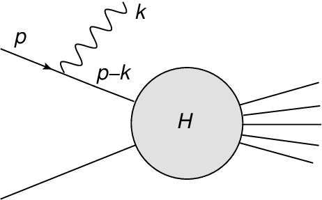
Figure 1: Diagrammatic representation of an external emission (left) and internal emission (right) in a scattering amplitude. The blob HH represents a generic subdiagram sensitive to the unspecified hard dynamics.

The factorization of two next-to-soft graviton emissions proceeds differently for external and internal emissions, as originally presented by Low in the gauge theory case [63, 64, 65, 66]. The difference between the two cases is better understood by looking at the diagrams in fig. 1 for a single next-to-soft boson.

More specifically, for one external emission, one considers a single line of momentum pip_{i} and simply expands the diagram at next-to-leading power in the soft graviton momentum kk. This amounts to either expanding the vertices in eq. 2.4, eq. 2.5 and the scalar propagator of momentum pi−kp_{i}-k, or to expanding the hard function as

H⁡(p1,…,pi−k,…,pn)=H⁡(p1,…,pi,…,pn)−kμ​∂∂pμ​H​(p1,…,pi,…,pn).\displaystyle H(p_{1},...,p_{i}-k,...,p_{n})=H(p_{1},...,p_{i},...,p_{n})-k_{\mu}\frac{\partial}{\partial p_{\mu}}H(p_{1},...,p_{i},...,p_{n})~. (2.6)

For an internal emission, on the other hand, one cannot naively compute the diagram in the right of fig. 1 due to the ignorance about the coupling of the soft boson with the hard subdiagram. Instead one exploits the gauge invariance of the full amplitude to express the result in terms of the external emission diagrams. For on-shell gravitons, the outcome is that the internal emission diagram and the derivative term in eq. 2.6 combine into a term consisting of the orbital angular momentum Lμ​ν=pμ​∂∂pν−pν​∂∂pμL^{\mu\nu}=p^{\mu}\frac{\partial}{\partial p^{\nu}}-p^{\nu}\frac{\partial}{\partial p^{\mu}} acting on the non-radiative amplitude. More generally, one can observe that the internal contribution is equal to an eikonal emission dressing the non-radiative amplitude with shifted kinematics [34, 56].

The contribution from the external emissions without derivatives acting on HH can be elaborated further. For example, for two emissions one sums over all possible graviton insertions on the scalar line, as shown in fig. 2. While for emissions of order κ\kappa this presents no difficulty, for contributions of order κ2\kappa^{2} the algebra is quite tedious and not shown here. Still, the result can be written in a relatively compact form in terms of three vertices:

Vμ​νE​(k)\displaystyle V^{\text{E}}_{\mu\nu}(k) =−κ2​pμ​pνp​k,\displaystyle=-\frac{\kappa}{2}\frac{p_{\mu}p_{\nu}}{pk}~, (2.7)
Vμ​νNE​(k)\displaystyle V^{\text{NE}}_{\mu\nu}(k) =−κ4​k2​pμ​pν(p​k)2+κ4​1p​k​(kμ​pν+kν​pμ−ημ​ν​p​k),\displaystyle=-\frac{\kappa}{4}\frac{k^{2}p_{\mu}p_{\nu}}{(pk)^{2}}+\frac{\kappa}{4}\frac{1}{pk}(k_{\mu}p_{\nu}+k_{\nu}p_{\mu}-\eta_{\mu\nu}pk)~, (2.8)
Vμ​ν​ρ​σNE​(k,l)\displaystyle V^{\text{NE}}_{\mu\nu\rho\sigma}(k,l) =κ241p⁡(k+l)[k​lp​k​p​lpμpνpρpσ−pρ​pσp​l(pμlν+pνlμ)−pμ​pνp​k(pρkσ+pσkρ)\displaystyle=\frac{\kappa^{2}}{4}\frac{1}{p(k+l)}\Bigg[\frac{kl}{pk~pl}p_{\mu}p_{\nu}p_{\rho}p_{\sigma}-\frac{p_{\rho}p_{\sigma}}{pl}(p_{\mu}l_{\nu}+p_{\nu}l_{\mu})-\frac{p_{\mu}p_{\nu}}{pk}(p_{\rho}k_{\sigma}+p_{\sigma}k_{\rho})
+ημ​ρpσpν+ην​ρpσpμ+ημ​σpρpν+ην​σpρpμ],\displaystyle\qquad+\eta_{\mu\rho}p_{\sigma}p_{\nu}+\eta_{\nu\rho}p_{\sigma}p_{\mu}+\eta_{\mu\sigma}p_{\rho}p_{\nu}+\eta_{\nu\sigma}p_{\rho}p_{\mu}\Bigg]~, (2.9)

where kk and ll denote the soft momenta. The first vertex represents the well-known single-graviton eikonal (E) Feynman rule, already present in Weinberg’s theorem [67], while the next-to-eikonal (NE) correction is given by Vμ​νNEV^{\text{NE}}_{\mu\nu} 33 3 Note that the contribution from Vμ​νNEV^{\text{NE}}_{\mu\nu} vanishes for on-shell gravitons in de Donder gauge (i.e. when 12​∂μh−∂νhμ​ν=0\frac{1}{2}\partial^{\mu}h-\partial_{\nu}h^{\mu\nu}=0), in agreement with the next-to-soft theorems of [68]. However, applications in high-energy scattering require off-shell gravitons. In that case, the second term in eq. 2.8 brings a non-vanishing correction to the Regge trajectory [56]. . At subleading order we should consider also a two-graviton seagull-like vertex, given by Vμ​ν​ρ​σNEV^{\text{NE}}_{\mu\nu\rho\sigma}.

Refer to caption
Figure 2: Factorization of two graviton emissions of momenta k1k_{1} and k2k_{2} at order κ2\kappa^{2}. Diagrams on the l.h.s. are constructed with the full vertices of eq. 2.4 and eq. 2.5 and then expanded at next-to soft level. The diagrams on the r.h.s. instead contain the combined vertex-propagator Feynman rules of eq. 2.7, eq. 2.8 and eq. 2.9. Next-to-eikonal emissions are denoted with a blob.

The question is whether this factorization persists at every order in κ\kappa, i.e. whether the sum of all possible attachments of NN gravitons emissions at next-to-soft level can be written exclusively in terms of the vertices of eq. 2.7, eq. 2.8 and eq. 2.9. As we are going to discuss, the GWL is meant to implement this idea by achieving an exponentiation along the hard particle worldline.

3 GWL from four-dimensional field theory

The derivation of the GWL from the field theory Lagrangian has been already discussed in detail in [53] after defining the graviton field via

g​gμ​ν=ημ​ν+κ​hμ​ν.\displaystyle\sqrt{g}g_{\mu\nu}=\eta_{\mu\nu}+\kappa h_{\mu\nu}~. (3.1)

In order to highlight the main points that will be addressed in the worldline approach of the next sections, here we revisit the approach of [53] to derive the GWL. In particular, we use the weak field expansion of eq. 1.2, which is more common in the literature, instead of eq. 3.1. In fact, it is worth noting that, unlike in gauge theories, gravitational GWLs are sensitive to how the graviton field is defined via the weak field expansion. Also, we use a mostly minus metric throughout.

We begin with the Schwinger representation of the dressed propagator. We first take eq. 2.1 and perform the weak field expansion with eq. 1.2, eq. 2.2 and eq. 2.3. Then, after integrating by parts and neglecting the surface term, eq. 2.1 becomes

S\displaystyle S =∫ddxϕ∗(x)(□+m2+κ[−∂μ∂νhμ​ν+∂ν(∂μhμ​ν)+(□+m2)h2−12∂μ(∂μh)]\displaystyle=\int d^{d}x\,\phi^{*}(x)\Bigg(\Box+m^{2}+\kappa\left[-\partial^{\mu}\partial^{\nu}h_{\mu\nu}+\partial^{\nu}(\partial^{\mu}h_{\mu\nu})+(\Box+m^{2})\frac{h}{2}-\frac{1}{2}\partial_{\mu}(\partial^{\mu}h)\right]
+κ2[(□+m2)(h28−hμ​ν24)−∂μ(∂μ(h28−hμ​ν24))−∂μ∂νh2hμ​ν\displaystyle\quad+\kappa^{2}\Bigg[(\Box\!+\!m^{2})\left(\frac{h^{2}}{8}\!-\!\frac{h_{\mu\nu}^{2}}{4}\right)\!-\partial^{\mu}\left(\!\partial_{\mu}\!\left(\frac{h^{2}}{8}\!-\!\frac{h_{\mu\nu}^{2}}{4}\right)\!\right)-\!\partial^{\mu}\partial^{\nu}\frac{h}{2}h_{\mu\nu}\!
+∂νh2(∂μhμ​ν)+∂ν(∂μh2)hμ​ν+∂μ∂νhρμhρ​ν−∂μ(∂νhρμhρ​ν)])ϕ(x).\displaystyle\quad+\!\partial^{\nu}\frac{h}{2}(\partial^{\mu}h_{\mu\nu})\!+\partial^{\nu}\!(\partial^{\mu}\frac{h}{2})h_{\mu\nu}+\partial_{\mu}\partial_{\nu}h^{\mu}_{\rho}h^{\rho\nu}-\partial_{\mu}(\partial_{\nu}h^{\mu}_{\rho}h^{\rho\nu})\Bigg]\Bigg)\phi(x)~. (3.2)

By writing eq. 3.2 in the form ∫d4​x​ϕ∗​(2​H)​ϕ\int d^{4}x\,\phi^{*}(2H)\phi, we can define 2​H2H as the inverse scalar propagator dressed with gravitational radiation. The Schwinger representation of this propagator consists of interpreting HH as a Hamiltonian governing the evolution in proper time TT of a relativistic scalar particle. This is achieved by first replacing all derivatives in HH acting on a wave function via i∂μ→p^μi\partial_{\mu}\to\hat{p}_{\mu}. Hence, in p​xpx-ordering (i.e. with all momentum operators on the left of the position operator) the Hamiltonian reads

H^=\displaystyle\hat{H}= −12​(p2−m2+κ⁡[−pμ​pν​hμ​ν+i​pν​(∂μhμ​ν)+12​(p2−m2)​h−i2​pμ​(∂μh)]CLOSE\displaystyle-\frac{1}{2}\Bigg(p^{2}-m^{2}+\kappa\left[-p^{\mu}p^{\nu}h_{\mu\nu}+ip^{\nu}(\partial^{\mu}h_{\mu\nu})+\frac{1}{2}(p^{2}-m^{2})h-\frac{i}{2}p_{\mu}(\partial^{\mu}h)\right]
+κ2[(p2−m2)(h28−hμ​ν24)−ipμ∂μ(h28−hμ​ν24)−12pμpνhμ​νh\displaystyle+\kappa^{2}\!\Bigg[(p^{2}-m^{2})\left(\frac{h^{2}}{8}-\frac{h_{\mu\nu}^{2}}{4}\right)\!-ip^{\mu}\partial_{\mu}\!\left(\frac{h^{2}}{8}\!-\!\frac{h_{\mu\nu}^{2}}{4}\right)\!-\frac{1}{2}p^{\mu}p^{\nu}h_{\mu\nu}h\!
+i2pνh(∂μhμ​ν)+i2pν(∂μh)hμ​ν+pμpνhρμhρ​ν−ipμ(∂νhρμhρ​ν)])+𝒪(κ3).\displaystyle+\!\frac{i}{2}p^{\nu}h(\partial^{\mu}h_{\mu\nu})\!+\!\frac{i}{2}p^{\nu}\left(\partial^{\mu}h\right)h_{\mu\nu}+p_{\mu}p_{\nu}h^{\mu}_{\rho}h^{\rho\nu}-ip_{\mu}(\partial_{\nu}h^{\mu}_{\rho}h^{\rho\nu})\Bigg]\Bigg)+{\cal O}(\kappa^{3})~. (3.3)

The dressed propagator in position representation then becomes

⟨xf|(2i(H−iϵ))−1|xi⟩=12∫0∞dT⟨xf|e−i⁡(H−i​ϵ)​T|xi⟩=∫0∞dT∫x⁡(0)=xix⁡(T)=xf𝒟x𝒟pe−i∫0Tdt(px˙+H(x,p)−iϵ),\displaystyle\langle{x_{f}}|(2i(H-i\epsilon))^{-1}|{x_{i}}\rangle=\frac{1}{2}\int\limits_{0}^{\infty}dT~\langle{x_{f}}|e^{-i(H-i\epsilon)T}|{x_{i}}\rangle=\int\limits_{0}^{\infty}dT\int\limits\displaylimits_{x(0)=x_{i}}^{x(T)=x_{f}}\mathcal{D}x\,\mathcal{D}p\,e^{-i\int\limits_{0}^{T}dt(p\dot{x}+H(x,p)-i\epsilon)}~, (3.4)

where we inserted the standard Feynman i​ϵi\epsilon prescription, and in the second step we used a path integral representation for the matrix elements.

In the following, we will be interested in solving eq. 3.4 order by order in the soft expansion in the asymptotic limit. To do so, we need to Fourier transform eq. 3.4 before carrying out the path integral over xx. This can be done by considering the transition element from an initial state of position xix_{i} to a final state of momentum pfp_{f}. The asymptotic propagator is then defined as the dressed propagator truncated of the external free propagator of momentum pfp_{f}. After performing the Gaussian momentum integration in eq. 3.4 and expanding around the classical solutions x=xi+pf​t+x~x=x_{i}+p_{f}t+\tilde{x}, the asymptotic propagator reads

−i(pf2−m2+iϵ)⟨pf|(2i(H−iϵ))−1|xi⟩=−i(pf2−m2+iϵ)∫0∞dTei​pf​xi−i2​(pf2−m2+i​ϵ)​Tf(T).-i(p_{f}^{2}-m^{2}+i\epsilon)\,\bra{p_{f}}(2i(H-i\epsilon))^{-1}\ket{x_{i}}=-i(p_{f}^{2}-m^{2}+i\epsilon)\int_{0}^{\infty}dT\,e^{ip_{f}x_{i}-\frac{i}{2}(p_{f}^{2}-m^{2}+i\epsilon)T}\,f(T)~. (3.5)

Here we defined

f⁡(T)≡∫x~​(0)=0𝒟​x~​exp⁡(i​∫0Td​t​L​[x~​(t)]),\displaystyle f(T)\equiv\int\limits_{\tilde{x}(0)=0}\mathcal{D}\tilde{x}\exp\left(i\int\limits_{0}^{T}dt\,L[\tilde{x}(t)]\right)~, (3.6)

where

L⁡[x⁡(t)]\displaystyle L[x(t)] =−λ​x˙22+κ2[−λhμ​νpμpν+i(∂μhμ​νpν−12∂μhpμ)+\displaystyle=-\frac{\lambda\dot{x}^{2}}{2}+\frac{\kappa}{2}\Bigg[-\lambda h_{\mu\nu}p^{\mu}p^{\nu}+i\left(\partial^{\mu}h_{\mu\nu}p^{\nu}-\frac{1}{2}\partial_{\mu}hp^{\mu}\right)+
+λx˙μ(−2hμ​νpν+hpμ)+ix˙μ(∂νhμ​ν−12∂μh)+λx˙μx˙ν(h2ημ​ν−hμ​ν)]\displaystyle+\lambda\dot{x}^{\mu}\left(-2h_{\mu\nu}p^{\nu}+hp_{\mu}\right)+i\dot{x}^{\mu}\left(\partial^{\nu}h_{\mu\nu}-\frac{1}{2}\partial_{\mu}h\right)+\lambda\dot{x}^{\mu}\dot{x}^{\nu}\left(\frac{h}{2}\eta_{\mu\nu}-h_{\mu\nu}\right)\Bigg]
+κ24[λ(hhμ​νpμpν−h22m2)+i(hρ​σ∂μhρ​σpμ−2pν(∂ρhμ​ν)hμ​ρ)+\displaystyle+\frac{\kappa^{2}}{4}\Bigg[\lambda\left(hh_{\mu\nu}p^{\mu}p^{\nu}-\frac{h^{2}}{2}m^{2}\right)+i\left(h_{\rho\sigma}\partial^{\mu}h_{\rho\sigma}p_{\mu}-2p^{\nu}(\partial^{\rho}h_{\mu\nu})h_{\mu\rho}\right)+
+1λ​(18​∂μh​∂μh+12​∂νhμ​ν​∂ρhμ​ρ−12​∂μh​∂νhμ​ν)+\displaystyle~~~~~~~~+\frac{1}{\lambda}\left(\frac{1}{8}\partial_{\mu}h\partial^{\mu}h+\frac{1}{2}\partial^{\nu}h_{\mu\nu}\partial^{\rho}h_{\mu\rho}-\frac{1}{2}\partial_{\mu}h\partial^{\nu}h_{\mu\nu}\right)+
+λ​x˙μ​(−h22​pμ−hμ​ν2​pμ+2​h​hμ​ν​pν)+i​x˙μ​(−2​(∂ρhμ​ν)​hν​ρ+hρ​ν​∂μhρ​ν)\displaystyle~~~~~~~~+\lambda\dot{x}^{\mu}\left(-\frac{h^{2}}{2}p_{\mu}-h_{\mu\nu}^{2}p_{\mu}+2hh_{\mu\nu}p^{\nu}\right)+i\dot{x}^{\mu}\left(-2(\partial^{\rho}h_{\mu\nu})h_{\nu\rho}+h_{\rho\nu}\partial_{\mu}h_{\rho\nu}\right)
+λx˙μx˙ν(−(h22+hμ​ν2)ημ​ν+hhμ​ν)].\displaystyle~~~~~~~~+\lambda\dot{x}^{\mu}\dot{x}^{\nu}\left(-\left(\frac{h^{2}}{2}+h_{\mu\nu}^{2}\right)\eta_{\mu\nu}+hh_{\mu\nu}\right)\Bigg]~. (3.7)

Note that in eq. 3.7 we have introduced a bookkeeping parameter λ\lambda and rescaled p→λ​pp\to\lambda p, t→t/λt\to t/\lambda and κ→κ/λ\kappa\to\kappa/\lambda. This choice is convenient in order to perform the soft expansion as a Laurent expansion in 1/λ1/\lambda.

Eq.(3.5) can be elaborated further by following a series of manipulations first described in [52]. Indeed, since the dressed propagator ⟨pf|​(2​i​(H−i​ϵ))−1​|xi⟩\bra{p_{f}}(2i(H-i\epsilon))^{-1}\ket{x_{i}} in the on-shell limit develops a simple pole with residue one and because the factor f⁡(T)f(T) remains finite in this limit, we can integrate by parts to get

(pf2−m2+i​ϵ)​⟨pf|​(2​i​(H−i​ϵ))−1​|xi⟩\displaystyle(p_{f}^{2}-m^{2}+i\epsilon)\,\bra{p_{f}}(2i(H-i\epsilon))^{-1}\ket{x_{i}} =ei​pf​xi​∫0∞d​T​(dd​T​e−i2​(pf2−m2)​T)​e−ϵ​T​f​(T)\displaystyle=e^{ip_{f}x_{i}}\int_{0}^{\infty}dT\,\left(\frac{d}{dT}e^{-\frac{i}{2}(p_{f}^{2}-m^{2})T}\right)\,e^{-\epsilon T}f(T)
=\displaystyle= ei​pf​xi​(−f⁡(0)−∫0∞d​T​e−i2​(pf2−m2)​T​dd​T​(e−ϵ​T​f​(T)))\displaystyle e^{ip_{f}x_{i}}\left(-f(0)-\int_{0}^{\infty}dT\,e^{-\frac{i}{2}(p_{f}^{2}-m^{2})T}\,\frac{d}{dT}\left(e^{-\epsilon T}f(T)\right)\right)
=\displaystyle= ei​pf​xi​limT→∞e−ϵ​T​f​(T),\displaystyle e^{ip_{f}x_{i}}\lim_{T\to\infty}e^{-\epsilon T}f(T)~, (3.8)

where in the last step we took the on-shell limit pf2→m2p_{f}^{2}\to m^{2}. Therefore, eq. 3.5 reads

(pf2−m2+i​ϵ)​⟨pf|​(2​i​(H−i​ϵ))−1​|xi⟩=ei​pf​xi​∫x~​(0)=0𝒟​x~​exp⁡(i​∫0∞d​t​e−ϵ​t​L​[x~​(t)]).(p_{f}^{2}-m^{2}+i\epsilon)\,\bra{p_{f}}(2i(H-i\epsilon))^{-1}\ket{x_{i}}=e^{ip_{f}x_{i}}\int\limits_{\tilde{x}(0)=0}\mathcal{D}\tilde{x}\exp\left(i\int\limits_{0}^{\infty}dt~e^{-\epsilon t}L[\tilde{x}(t)]\right)~. (3.9)

A few comments are in order. Since the graviton field is a function of the spacetime variable xμ​(t)=xi+pf​t+x~​(t)x^{\mu}(t)=x_{i}+p_{f}t+\tilde{x}(t), the Lagrangian in eq. 3.7 and eq. 3.9 defines a one-dimensional quantum field theory for the field x~μ​(t)\tilde{x}^{\mu}(t), representing the fluctuations in the trajectory of the scalar particle due to graviton emissions. As first noted in [52], it is convenient to evaluate the path integral for xi=0x_{i}=0. The effect of having xi≠0x_{i}\neq 0 is computed separately and, after combining it with the internal emission discussed in section 2, yields a combination of derivatives of the non-radiative process, which corresponds to a coupling with the orbital angular momentum of the scalar particle.

Path integrals like in eq. 3.9 are typically solved in the worldline formalism at the amplitude level, i.e. after combining all dressed propagators of the amplitude. In this way one obtains master formulae that generate integral representations of the amplitude order by order in the coupling constant κ\kappa, corresponding to a fixed number of graviton emissions. The GWL approach is different. In the gauge theory case the GWL is constructed from the evaluation of the equivalent expression to eq. 3.9 for each asymptotic particle, order by order in the soft expansion (i.e. assuming the soft momentum k≪pfk\ll p_{f}) but considering an arbitrary number of soft emissions. In this way, the worldline path integral is solved once for each external scalar line, while the amplitude is constructed in terms of vacuum expectation values of GWLs using the action governing the background field. The same approach can be implemented in gravity, with some complication due to the presence of the weak field expansion. In fact, while one has still k≪pfk\ll p_{f}, higher orders in κ\kappa are also suppressed, which can be seen as a consequence of the charge being the four-momentum.

To avoid ambiguities between the weak and soft expansions, in eq. 3.7 we have introduced a single bookkeeping parameter λ\lambda and rescaled p→λ​pp\to\lambda p, t→t/λt\to t/\lambda and κ→κ/λ\kappa\to\kappa/\lambda. In this way, the path integral is evaluated order by order in 1/λ1/\lambda. To see why this is possible, one can observe that expanding the background field hμ​ν​(pf​t+x)h^{\mu\nu}(p_{f}t+x) around pf​tp_{f}t generates powers of xx with no λ\lambda enhancement. On the other hand, two-point correlators of xx are of order 1/λ1/\lambda, and are given by

    ​xμ​(t)​xν​(t′)\displaystyle\mathchoice{\vbox{\hbox to0.0pt{\kern 0.0pt\kern 11.23325pt\hbox{\vrule width=0.50003pt,height=0.0pt,depth=4.30554pt\vrule width=23.44276pt,height=0.0pt,depth=0.50003pt\vrule width=0.50003pt,height=0.0pt,depth=4.30554pt}\hss}\vskip 2.15277pt\vskip 7.5pt}}{\vbox{\hbox to0.0pt{\kern 0.0pt\kern 11.23325pt\hbox{\vrule width=0.50003pt,height=0.0pt,depth=4.30554pt\vrule width=23.44276pt,height=0.0pt,depth=0.50003pt\vrule width=0.50003pt,height=0.0pt,depth=4.30554pt}\hss}\vskip 2.15277pt\vskip 7.5pt}}{\vbox{\hbox to0.0pt{\kern 0.0pt\kern 9.27724pt\hbox{\vrule width=0.50003pt,height=0.0pt,depth=4.30554pt\vrule width=19.56259pt,height=0.0pt,depth=0.50003pt\vrule width=0.50003pt,height=0.0pt,depth=4.30554pt}\hss}\vskip 2.15277pt\vskip 5.25pt}}{\vbox{\hbox to0.0pt{\kern 0.0pt\kern 8.47113pt\hbox{\vrule width=0.50003pt,height=0.0pt,depth=4.30554pt\vrule width=17.95038pt,height=0.0pt,depth=0.50003pt\vrule width=0.50003pt,height=0.0pt,depth=4.30554pt}\hss}\vskip 2.15277pt\vskip 3.75pt}}x_{\mu}(t)x_{\nu}(t^{\prime}) =−iλ​min⁡(t,t′)​ημ​ν,\displaystyle=\frac{-i}{\lambda}\min(t,t^{\prime})\eta_{\mu\nu}~, (3.10)
    ​x˙μ​(t)​xν​(t′)\displaystyle\mathchoice{\vbox{\hbox to0.0pt{\kern 0.0pt\kern 9.76451pt\hbox{\vrule width=0.50003pt,height=0.0pt,depth=4.30554pt\vrule width=21.97401pt,height=0.0pt,depth=0.50003pt\vrule width=0.50003pt,height=0.0pt,depth=4.30554pt}\hss}\vskip 2.15277pt\vskip 7.5pt}}{\vbox{\hbox to0.0pt{\kern 0.0pt\kern 9.76451pt\hbox{\vrule width=0.50003pt,height=0.0pt,depth=4.30554pt\vrule width=21.97401pt,height=0.0pt,depth=0.50003pt\vrule width=0.50003pt,height=0.0pt,depth=4.30554pt}\hss}\vskip 2.15277pt\vskip 7.5pt}}{\vbox{\hbox to0.0pt{\kern 0.0pt\kern 8.39877pt\hbox{\vrule width=0.50003pt,height=0.0pt,depth=4.30554pt\vrule width=18.68413pt,height=0.0pt,depth=0.50003pt\vrule width=0.50003pt,height=0.0pt,depth=4.30554pt}\hss}\vskip 2.15277pt\vskip 6.67859pt}}{\vbox{\hbox to0.0pt{\kern 0.0pt\kern 7.88084pt\hbox{\vrule width=0.50003pt,height=0.0pt,depth=4.30554pt\vrule width=17.36009pt,height=0.0pt,depth=0.50003pt\vrule width=0.50003pt,height=0.0pt,depth=4.30554pt}\hss}\vskip 2.15277pt\vskip 6.67859pt}}\dot{x}_{\mu}(t)x_{\nu}(t^{\prime}) =−iλ​θ​(t′−t)​ημ​ν,\displaystyle=\frac{-i}{\lambda}\theta(t^{\prime}-t)\eta_{\mu\nu}~, (3.11)
    ​x˙μ​(t)​x˙ν​(t′)\displaystyle\mathchoice{\vbox{\hbox to0.0pt{\kern 0.0pt\kern 9.76451pt\hbox{\vrule width=0.50003pt,height=0.0pt,depth=4.30554pt\vrule width=20.50528pt,height=0.0pt,depth=0.50003pt\vrule width=0.50003pt,height=0.0pt,depth=4.30554pt}\hss}\vskip 2.15277pt\vskip 7.5pt}}{\vbox{\hbox to0.0pt{\kern 0.0pt\kern 9.76451pt\hbox{\vrule width=0.50003pt,height=0.0pt,depth=4.30554pt\vrule width=20.50528pt,height=0.0pt,depth=0.50003pt\vrule width=0.50003pt,height=0.0pt,depth=4.30554pt}\hss}\vskip 2.15277pt\vskip 7.5pt}}{\vbox{\hbox to0.0pt{\kern 0.0pt\kern 8.39877pt\hbox{\vrule width=0.50003pt,height=0.0pt,depth=4.30554pt\vrule width=17.80565pt,height=0.0pt,depth=0.50003pt\vrule width=0.50003pt,height=0.0pt,depth=4.30554pt}\hss}\vskip 2.15277pt\vskip 6.67859pt}}{\vbox{\hbox to0.0pt{\kern 0.0pt\kern 7.88084pt\hbox{\vrule width=0.50003pt,height=0.0pt,depth=4.30554pt\vrule width=16.7698pt,height=0.0pt,depth=0.50003pt\vrule width=0.50003pt,height=0.0pt,depth=4.30554pt}\hss}\vskip 2.15277pt\vskip 6.67859pt}}\dot{x}_{\mu}(t)\dot{x}_{\nu}(t^{\prime}) =−iλ​δ​(t′−t)​ημ​ν.\displaystyle=\frac{-i}{\lambda}\delta(t^{\prime}-t)\eta_{\mu\nu}~. (3.12)

Therefore, only a finite number of diagrams is necessary at a given order in 1/λ1/\lambda. At this point, we note that equal-time correlators are ill-defined. The prescription used in [53] is to set to zero both θ⁡(t′−t)\theta(t^{\prime}-t) and δ⁡(t′−t)\delta(t^{\prime}-t) at equal time. In the following section we will discuss how this choice can be justified.

Although the weak field expansion differs from the one of [53], the calculation of the path integral in eq. 3.9 is essentially the same. However, the number of terms is greatly reduced. For the sake of completeness an explicit evaluation of the worldline diagrams is discussed in appendix A. The upshot is that the sum of the connected diagrams is equal to the sum of the terms in eq. 2.7, eq. 2.8 and eq. 2.9. It is worth mentioning that, as in [53], it is still necessary to expand the Hamiltonian up to order κ2\kappa^{2} in order to correctly reproduce these vertices. Thus, we conclude that this feature is not due to the particular definition of the graviton field in eq. 1.2 or eq. 3.1, but it is due to the fact that the Hamiltonian has been defined after a weak field expansion.

The final step consists of exponentiating the result obtained from the worldline diagrams. In fact, remembering the standard property valid for any QFT with commuting sources that the sum of connected diagrams exponentiates, one obtaines

(pf2−m2+i​ϵ)\displaystyle(p_{f}^{2}-m^{2}+i\epsilon) ⟨pf|​(2​i​(H−i​ϵ))−1​|0⟩=exp⁡(κ​∫dd​k(2​π)d​(Vμ​νE​(k)+Vμ​νNE​(k))​h~μ​ν​(k)CLOSE\displaystyle\,\bra{p_{f}}(2i(H-i\epsilon))^{-1}\ket{0}=\exp\Bigg(\kappa\int\frac{d^{d}k}{(2\pi)^{d}}\left(V_{\mu\nu}^{\text{E}}(k)+V_{\mu\nu}^{\text{NE}}(k)\right)\tilde{h}^{\mu\nu}(k)
+κ2∫dd​k(2​π)d∫dd​l(2​π)dVμ​ν​ρ​σNE(k,l)h~μ​ν(k)h~ρ​σ(l)),\displaystyle\qquad\qquad+\kappa^{2}\int\frac{d^{d}k}{(2\pi)^{d}}\int\frac{d^{d}l}{(2\pi)^{d}}V_{\mu\nu\rho\sigma}^{\text{NE}}(k,l)\tilde{h}^{\mu\nu}(k)\tilde{h}^{\rho\sigma}(l)\Bigg)~, (3.13)

where h~μ​ν\tilde{h}^{\mu\nu} denotes the Fourier transform of the graviton field, while Vμ​νEV_{\mu\nu}^{\text{E}}, Vμ​νNEV_{\mu\nu}^{\text{NE}} and Vμ​ν​ρ​σNEV_{\mu\nu\rho\sigma}^{\text{NE}} have been defined in eq. 2.7, eq. 2.8 and eq. 2.9. This proves the exponentiation of the next-to-soft vertices discussed in section 2, thus showing that the next-to-soft factorization of fig. 2 persists to all orders in κ\kappa. Finally, performing the inverse Fourier transform in the r.h.s. of eq. 3.13 one obtains the GWL in position space defined in eq. 1.1.

4 GWL from worldline model in curved space

One of the crucial ingredients of the derivation outlined in the previous section is the definition of the Hamiltonian in eq. 3.3, which is obtained after a weak field expansion in the field theory Lagrangian. This approach is not satisfactory for a number of reasons. The first one is that it runs into difficulties when one attempts to generalize the definition to spinning emitters, as already observed in the gauge theory case in [62]. Secondly, the need to expand the Hamiltonian to order κ2\kappa^{2} in order to reproduce the vertices in eq. 2.9 is somewhat unconventional compared to the standard worldline formulation where the two-graviton vertex is reproduced by the order κ\kappa terms in the Hamiltonian. Finally (and perhaps more importantly), the above construction hides non-trivial cancellations of UV divergences, which arise from the equal-time delta function in eq. 3.12. This issue has been thoroughly discussed in the literature, and it requires the use of ghost fields and regularization scheme dependent counterterms in the Hamiltonian. It is not clear from the previous construction how the Hamiltonian in eq. 3.3 is affected by the UV regularization and what the role of the ghost fields is in the evaluation of the exponentiated worldline diagrams. In this section, we will demonstrate that a first-principles derivation of the GWL in the worldline formalism and the identification of the correct Hamiltonian before any weak field expansion clarify the above issues. In this way the construction of the GWL is put on a firm basis.

4.1 Quantization in curved space

The quantization of a relativistic particle on curved spacetime has a long history44 4 For a comprehensive review see [69] and references therein.. Most of the difficulties revolve around the issue of a unique definition of an Hamiltonian operator, due to the presence of UV divergences in the worldline model and the lack of an unambiguous definition for the momentum operator in absence of translational invariance [57].

The reason for the presence of UV divergences is relatively simple. A particle in flat spacetime can be described by the following classical phase space action

S⁡[x,p]=∫d​t​(−pμ​x˙μ+e​H​(x,p)),S[x,p]=\int dt\,\left(-p_{\mu}\dot{x}^{\mu}+eH(x,p)\right)~, (4.1)

where the einbein ee is the Lagrange multiplier for the constraint H⁡(x,p)=0H(x,p)=0. After quantizing the constrained model à la Dirac, and gauge fixing e=Te=T, one obtains the usual Schwinger representation of the dressed propagator as in eq. 3.4. With most Hamiltonians the momentum can be integrated out exactly, so that the action in configuration space takes the form

S⁡[x]=∫0Td​t​(−12​ημ​ν​x˙μ​x˙ν+V⁡(x)),\displaystyle S[x]=\int\limits_{0}^{T}dt\left(-\frac{1}{2}\eta_{\mu\nu}\dot{x}^{\mu}\dot{x}^{\nu}+V(x)\right)~, (4.2)

where V⁡(x)V(x) can be derived from the Hamiltonian. When moving to curved space, the kinetic term becomes a non-linear sigma model of the type gμ​ν​(x)​x˙μ​x˙νg_{\mu\nu}(x)\dot{x}^{\mu}\dot{x}^{\nu}. Although superrenormalizable, some diagrams might contain UV divergences55 5 The presence of IR divergences in the worldline path integral is instead more subtle. They are typically regulated by the proper time TT. However, in the asymptotic limit one eventually takes the limit T→∞T\to\infty. This has the consequence that IR divergences show up in the vacuum expectation values of multiple GWLs, as expected.. More specifically, the divergences come from correlators of x˙​(t)\dot{x}(t) evaluated at equal time, a feature evident in eq. 3.12 in the previous section and also in four-dimensional theories [70].

As it is well-known [71], to solve the problem one needs to define a regularization prescription and to subsequently renormalize the divergences with suitable counterterms, with a scheme dependent finite remainder in this cancellation. Among the various regularization schemes, time slicing has the advantage that such cancellation is already built-in in the path integral measure. Indeed, integrating out the momentum yields a factor (−g(x))−1/2(-g(x))^{-1/2} that can be exponentiated in terms of ghost fields, whose correlators should cancel the divergences in ⟨x˙​(t)​x˙​(t)⟩\langle\dot{x}(t)\dot{x}(t)\rangle. Unlike in other methods, such as mode regularization or dimensional regularization, no counterterm must be inserted by hand, since the additional term in the Hamiltonian operator H^\hat{H} naturally arises from ordering the operators x^\hat{x} and p^\hat{p}.

Clearly, discussing the Hamiltonian ordering assumes that a suitable definition for H^\hat{H} has been found within a meaningful quantization procedure, as we now briefly review. We start by observing that the constraint H^​|ψ⟩=0\hat{H}|\psi\rangle=0 should be equivalent to the Klein-Gordon equation

(∇μgμ​ν∂ν+m2)ϕ(x)=0,\displaystyle(\nabla_{\mu}g^{\mu\nu}\partial_{\nu}+m^{2})\phi(x)=0~, (4.3)

where ∇μ\nabla_{\mu} denotes the covariant derivative. In this way, H^\hat{H} contains the covariant Laplacian and it is automatically invariant under general relativity transformations. Once a definition for the momentum operator p^\hat{p} in position representation is adopted, the Hamiltonian operator H^\hat{H} follows unambiguously. A common choice in the literature is given by

⟨x|p^μ|ψ⟩\displaystyle\langle x|\hat{p}_{\mu}|\psi\rangle =(−g(x^))−1/4(i∂μ)(−g(x^))1/4⟨x|ψ⟩,\displaystyle=(-g(\hat{x}))^{-1/4}(i\partial_{\mu})(-g(\hat{x}))^{1/4}\,\langle x|\psi\rangle~, (4.4)

which yields

2​H^\displaystyle 2\hat{H} =−(−g(x^))−1/4p^μgμ​ν(x^)−g⁡(x^)p^ν(−g(x^))−1/4+m2,\displaystyle=-(-g(\hat{x}))^{-1/4}\,\hat{p}_{\mu}\,g^{\mu\nu}(\hat{x})\,\sqrt{-g(\hat{x})}\,\hat{p}_{\nu}\,(-g(\hat{x}))^{-1/4}+m^{2}~, (4.5)

where the x^\hat{x} dependence has been made explicit. One can readily verify that the operator in eq. 4.4 is hermitian w.r.t. the Hilbert space inner product, defined as

⟨ψ|χ⟩\displaystyle\langle\psi|\chi\rangle =∫dd​x​−g​ψ∗​(x)​χ​(x),\displaystyle=\int d^{d}x\,\sqrt{-g}\,\psi^{*}(x)\chi(x)~, (4.6)

where we normalized the x^\hat{x} eigenstates via

1=∫dd​x​−g​|x⟩​⟨x|,⟨x|x′⟩=1−g​δ​(x−x′).\displaystyle 1=\int d^{d}x\,\sqrt{-g}\,|x\rangle\langle x|~,\qquad\langle x|x^{\prime}\rangle=\frac{1}{\sqrt{-g}}\delta(x-x^{\prime})~. (4.7)

Note that the definition in eq. 4.4 is consistent with the normalization ⟨x|p⟩=⟨p|x⟩†=(−g)−1/4e−i​pμ​xμ\langle x|p\rangle=\langle p|x\rangle^{{\dagger}}=(-g)^{-1/4}e^{-ip_{\mu}x^{\mu}}. This is particularly convenient in Weyl ordering, i.e. when symmetrizing all x^\hat{x} and p^\hat{p} operators.

In the construction of the GWL, on the other hand, the building block is the asymptotic propagator ⟨pf|e−i​H​t|xi⟩\langle p_{f}|e^{-iHt}|x_{i}\rangle, as we discussed in the previous section. Hence, even if we consider the position space dressed propagator, some kind of Fourier transform must be defined before taking the weak field expansion. In fact, although the dependence over the conjugate momentum pp is Gaussian and the non-trivial path integral is the one over xx, the latter is evaluated pertubatively in the soft expansion by adding fluctuations over the straight classical path in flat spacetime, via the scaling defined by the final momentum pfp_{f}. This asymmetry between initial and final state makes p​xpx-ordering preferable w.r.t Weyl ordering.

These considerations lead us to define the Fourier transform as 66 6 This definition has been extensively discussed in [72].

ψ~​(p)\displaystyle\tilde{\psi}(p) ≡⟨p|ψ⟩=∫dd​x​−g​ψ​(x)​ei​pμ​xμ,\displaystyle\equiv\langle p|\psi\rangle=\int d^{d}x\,\sqrt{-g}\,\psi(x)\,e^{ip_{\mu}x^{\mu}}, (4.8)

or equivalently we define the left eigenstates of p^\hat{p} via ⟨p|x⟩=ei​pμ​xμ\langle p|x\rangle=e^{ip_{\mu}x^{\mu}}. Using the normalization of eq. 4.7, it is easy to see that eq. 4.8 implies

⟨x|p^μ|ψ⟩\displaystyle\langle x|\hat{p}_{\mu}|\psi\rangle =(−g(x^))−1/2(i∂μ)(−g(x^))1/2⟨x|ψ⟩.\displaystyle=(-g(\hat{x}))^{-1/2}(i\partial_{\mu})(-g(\hat{x}))^{1/2}\,\langle x|\psi\rangle~. (4.9)

This definition is not hermitian w.r.t. the inner product of eq. 4.6. Note also that ⟨x|p⟩=(−g)−1/2e−i​pμ​xμ≠⟨p|x⟩†\langle x|p\rangle=(-g)^{-1/2}e^{-ip_{\mu}x^{\mu}}\neq\langle p|x\rangle^{{\dagger}} and that the wavefunction ψ~​(p)\tilde{\psi}(p) in eq. 4.8 is not a scalar in general relativity. However, the Hamiltonian must be invariant. In fact, by demanding that H^​|ψ⟩=0\hat{H}|\psi\rangle=0 returns eq. 4.3 with the momentum in eq. 4.9, the Hamiltonian is uniquely defined and reads

2​H^\displaystyle 2\hat{H} =−p^μgμ​ν(x^)(−g(x^))1/2p^ν(−g(x^))−1/2+m2.\displaystyle=-\hat{p}_{\mu}\,g^{\mu\nu}(\hat{x})\,(-g(\hat{x}))^{1/2}\,\hat{p}_{\nu}\,(-g(\hat{x}))^{-1/2}+m^{2}~. (4.10)

The non-hermitian result77 7 We stress that both the operator x^\hat{x} and the Hamiltonian in eq. 4.10 are hermitian. in eq. 4.9 (or equivalently the non-invariant Fourier transform defined in eq. 4.8) might seem puzzling at first sight but it is a direct consequence of p​xpx-ordering[73]. In fact, it does not pose any real problem, since the physical momentum contained in the GWL is the momentum pfp_{f} defined in flat spacetime and not the conjugate momentum p^\hat{p}. The reason for this choice can be appreciated only after defining the classical Hamiltonian Hp​x​(p,x)H_{px}(p,x) from eq. 4.10 in p​xpx-ordering, i.e.

2​Hp​x​(p,x)\displaystyle 2H_{px}(p,x) ≡−pμ​pν​gμ​ν+m2+i​pμ​(∂νgμ​ν+gμ​ν​(∂νln⁡(−g))).\displaystyle\equiv-p_{\mu}\,p_{\nu}\,g^{\mu\nu}+m^{2}+ip_{\mu}(\partial_{\nu}g^{\mu\nu}+g^{\mu\nu}(\partial_{\nu}\ln(\sqrt{-g})))~. (4.11)

The logarithmic term in eq. 4.11 contains the trace of the metric and cannot be generated in p​xpx-ordering with the hermitian definitions of eq. 4.4 and eq. 4.5, as one can readily verify. This term is crucial in order to correctly reproduce the two-graviton vertex, as we are going to discuss in section 4.3. Before doing that, we need to set up a path integral representation for the asymptotic propagator.

4.2 Setting up the path integral

Equipped with the Hamiltonian in eq. 4.11, we can now work out a path integral representation for the dressed propagator in time slicing regularization. In analogy with the discussion in section 3, we consider

⟨pf|​e−i⁡(H^−i​ϵ)​t​|xi⟩=\displaystyle\bra{p_{f}}e^{-i(\hat{H}-i\epsilon)t}\ket{x_{i}}=
=\displaystyle= ∫∏i=2Nd4​xi​−g⁡(xi)​∏j=1N−1d4​pi(2​π)4​∏n=1Nexp⁡(−i​Hp​x​(pn,xn)​τ)​⟨pn|xn⟩​∏m=1N−1⟨xm+1|pm⟩\displaystyle\int\limits\prod_{i=2}^{N}d^{4}x_{i}\sqrt{-g(x_{i})}\prod_{j=1}^{N-1}\frac{d^{4}p_{i}}{(2\pi)^{4}}\prod_{n=1}^{N}\exp\left(-iH_{px}(p_{n},x_{n})\tau\right)\braket{p_{n}|x_{n}}\prod_{m=1}^{N-1}\braket{x_{m+1}|p_{m}}
=\displaystyle= ei​pN​xN∫∏i=2Nd4xi∏j=1N−1d4​pi(2​π)4exp{−i∑n=1N−1pn(xn+1−xn)−i∑n=1NHp​x(pn,xn)τ−iϵ},\displaystyle e^{ip_{N}x_{N}}\int\limits\prod_{i=2}^{N}d^{4}x_{i}\prod_{j=1}^{N-1}\frac{d^{4}p_{i}}{(2\pi)^{4}}\exp\left\{-i\sum_{n=1}^{N-1}p_{n}(x_{n+1}-x_{n})-i\sum_{n=1}^{N}H_{px}(p_{n},x_{n})\tau-i\epsilon\right\}~, (4.12)

where we sliced the time domain in NN intervals of length τ=T/N\tau=T/N. Note that eq. 4.12 is consistent with the Fourier transform defined in eq. 4.8.

In order to carry out the Gaussian momentum integration, it is convenient to define

Vnμ\displaystyle V^{\mu}_{n} ≡∂νgμ​ν​(xn)+gμ​ν​(xn)​(∂νln⁡(−g⁡(xn))),\displaystyle\equiv\partial_{\nu}g^{\mu\nu}(x_{n})+g^{\mu\nu}(x_{n})(\partial_{\nu}\ln(\sqrt{-g(x_{n})}))~, (4.13)
Bnμ\displaystyle B^{\mu}_{n} ≡−i​τ​[(xn+1−xn)μτ+i2​Vnμ].\displaystyle\equiv-i\tau\left[\frac{(x_{n+1}-x_{n})^{\mu}}{\tau}+\frac{i}{2}V_{n}^{\mu}\right]~. (4.14)

Then, eq. 4.12 becomes

⟨pf|​e−i⁡(H^−i​ϵ)​t​|xi⟩=ei​pN​xN−i2​m2​T​∫∏i=2Nd4​xi​(∏j=1N−1g⁡(xj)(2​π​τ)n)​exp⁡{i2​τ​∑n=1N−1Bnμ​gμ​νn​Bnν}.\bra{p_{f}}e^{-i(\hat{H}-i\epsilon)t}\ket{x_{i}}=e^{ip_{N}x_{N}-\frac{i}{2}m^{2}T}\int\limits\prod_{i=2}^{N}d^{4}x_{i}\left(\prod_{j=1}^{N-1}\sqrt{\frac{g(x_{j})}{(2\pi\tau)^{n}}}\right)\exp\left\{\frac{i}{2\tau}\sum_{n=1}^{N-1}B^{\mu}_{n}g_{\mu\nu}^{n}B^{\nu}_{n}\right\}. (4.15)

As anticipated in section 4.1, we can get rid of the determinants in the xx-measure by re-exponentiating them using three ghost fields, to get

⟨pf|​e−i⁡(H^−i​ϵ)​t​|xi⟩=ei​pN​xN−i2​m2​T​∫∏i=2Nd4​xi(2​π​τ)n​exp⁡{i2​τ​∑n=1N−1gμ​νn​Bnμ​Bnν}⋅Zg​h​o​s​t​s,\bra{p_{f}}e^{-i(\hat{H}-i\epsilon)t}\ket{x_{i}}=e^{ip_{N}x_{N}-\frac{i}{2}m^{2}T}\int\limits\prod_{i=2}^{N}\frac{d^{4}x_{i}}{(2\pi\tau)^{n}}\exp\left\{\frac{i}{2\tau}\sum_{n=1}^{N-1}g_{\mu\nu}^{n}B^{\mu}_{n}B^{\nu}_{n}\right\}\cdot Z_{ghosts}~, (4.16)

where Zg​h​o​s​t​sZ_{ghosts} reads

Zg​h​o​s​t​s=∫∏i=1N−1d4aid4bid4ciexp{−iτ2∑n=1N−1gμ​νn(anμanν+bnμcnν)},Z_{ghosts}=\int\limits\prod_{i=1}^{N-1}d^{4}a_{i}d^{4}b_{i}d^{4}c_{i}\exp\left\{-i\frac{\tau}{2}\sum_{n=1}^{N-1}g_{\mu\nu}^{n}(a_{n}^{\mu}a_{n}^{\nu}+b^{\mu}_{n}c^{\nu}_{n})\right\}, (4.17)

where as usual we have neglected irrelevant field-independent normalization constants. Here, aia_{i} are real commuting fields, while bib_{i} and cic_{i} are anti-commuting Grassmann fields.

The continuum limit of eq. 4.16 and eq. 4.17 follows straightforwardly. Expanding around the classical path x⁡(t)=xi+pf​t+x~​(t)x(t)=x_{i}+p_{f}\,t+\tilde{x}(t) and truncating the external free propagator, we obtain a path integral representation for the asymptotic propagator in analogy with eq. 3.9, i.e.

(pf2−m2+i​ϵ)​⟨pf|​(2​i​(H−i​ϵ))−1​|xi⟩=ei​pf​xi​∫x~​(0)=0𝒟​x~​𝒟​a​𝒟​b​𝒟​c​exp⁡(i​∫0∞d​t​e−ϵ​t​L​[x~,a,b,c]),(p_{f}^{2}-m^{2}+i\epsilon)\,\bra{p_{f}}(2i(H-i\epsilon))^{-1}\ket{x_{i}}=e^{ip_{f}x_{i}}\int\limits_{\tilde{x}(0)=0}\mathcal{D}\tilde{x}\mathcal{D}a\mathcal{D}b\mathcal{D}c\exp\left(i\int\limits_{0}^{\infty}dt~e^{-\epsilon t}~L[\tilde{x},a,b,c]\right)~, (4.18)

where the Lagrangian L⁡[x~,a,b,c]L[\tilde{x},a,b,c] reads

L⁡[x~,a,b,c]=−12​((x~˙μ​x~˙ν+aμ​aν+bμ​cν)​gμ​ν+i​(x~˙+pf)μ​gμ​ν​Vν−14​Vμ​gμ​ν​Vν).\displaystyle L[\tilde{x},a,b,c]=-\frac{1}{2}\left((\dot{\tilde{x}}^{\mu}\dot{\tilde{x}}^{\nu}+{a}^{\mu}{a}^{\nu}+{b}^{\mu}{c}^{\nu})g_{\mu\nu}+i(\dot{\tilde{x}}+p_{f})^{\mu}g_{\mu\nu}V^{\nu}-\frac{1}{4}V^{\mu}g_{\mu\nu}V^{\nu}\right)~. (4.19)

We stress that although we have expressed the path integral in terms of the classical straight solution in flat space, so far we have not performed any weak field expansion. Hence, the expression in eq. 4.19 holds for a generic curved background, as long as the Fourier transform of eq. 4.8 is meaningful.

At this point one would like to solve the path integral perturbatively, hence the need for the weak field expansion of eq. 1.2. While vertices can be read immediately from eq. 4.19, two-point correlators for all fields must be derived from the discrete version in eq. 4.16 and eq. 4.17 in order to avoid ambiguities at equal-time. Although similar calculations have been thoroughly discussed in the literature (see e.g. [69]), given the non-standard conventions required by the GWL (i.e. p​xpx-ordering and the asymptotic limit), and the quite laborious algebra, we present the corresponding derivation in appendix B. The upshot is that the propagators for the ghost fields read

⟨aμ​(t)​aν​(t′)⟩\displaystyle\langle a^{\mu}(t)a^{\nu}(t^{\prime})\rangle =−i​ημ​ν​δ​(t−t′),\displaystyle=-i\eta^{\mu\nu}\delta(t-t^{\prime})~, (4.20)
⟨bμ​(t)​cν​(t′)⟩\displaystyle\langle b^{\mu}(t)c^{\nu}(t^{\prime})\rangle =2​i​ημ​ν​δ​(t−t′),\displaystyle=2i\eta^{\mu\nu}\delta(t-t^{\prime})~, (4.21)

while the two-point correlators for the xμx^{\mu} fields assume exactly the same form as in eq. 3.10, eq. 3.11 and eq. 3.12. This time, however, their equal-time expression is non-ambiguous and follows from the regularization scheme. In particular, we obtain

⟨x˙μ​(t)​xν​(t)⟩\displaystyle\langle\dot{x}^{\mu}(t)x^{\nu}(t)\rangle =0,\displaystyle=0~, (4.22)
⟨x˙μ​(t)​x˙ν​(t)⟩\displaystyle\langle\dot{x}^{\mu}(t)\dot{x}^{\nu}(t)\rangle =−i​ημ​ν​δ​(0),\displaystyle=-i\eta^{\mu\nu}\delta(0)~, (4.23)
⟨aμ​(t)​aν​(t)⟩\displaystyle\langle a^{\mu}(t)a^{\nu}(t)\rangle =−i​ημ​ν​δ​(0),\displaystyle=-i\eta^{\mu\nu}\delta(0)~, (4.24)
⟨bμ​(t)​cν​(t)⟩\displaystyle\langle b^{\mu}(t)c^{\nu}(t)\rangle =2​i​ημ​ν​δ​(0).\displaystyle=2i\eta^{\mu\nu}\delta(0)~. (4.25)

This simple result shows that the correlator ⟨x˙μ​(t)​x˙ν​(t)⟩\langle\dot{x}^{\mu}(t)\dot{x}^{\nu}(t)\rangle is divergent in time slicing, but that the divergence is compensated by the ghost correlators ⟨aμ​(t)​aν​(t)⟩\langle a^{\mu}(t)a^{\nu}(t)\rangle and ⟨bμ​(t)​cν​(t)⟩\langle b^{\mu}(t)c^{\nu}(t)\rangle, in agreement with similar calculations in Weyl-ordering. On the other hand, unlike in Weyl-ordering, we do not obtain the midpoint rule ⟨x˙μ​(t)​xν​(t)⟩=θ⁡(0)​ημ​ν=1/2​ημ​ν\langle\dot{x}^{\mu}(t)x^{\nu}(t)\rangle=\theta(0)\,\eta^{\mu\nu}=1/2\,\eta^{\mu\nu} 88 8 This difference can be noted also in the gauge theory case discussed in [52] and [62]. There, one uses θ⁡(0)=0\theta(0)=0 while the next-to-soft vertex kμ/2​p⋅kk^{\mu}/2p\cdot k, analogous to eq. 2.8 in this paper, is due to the term ∂μAμ\partial_{\mu}A^{\mu} in the p​xpx-ordered Hamiltonian. This term is absent in Weyl-ordering, but the equal-time correlator ⟨x˙​(t)​x​(t)⟩\langle\dot{x}(t)x(t)\rangle is non-vanishing and compensates for the mismatch. . However, one should not be fooled by the simplicity of the results of eqs. 4.22 to 4.25 which hide some non-trivial manipulations in the discrete case, as shown in appendix B and appendix C.

The soft expansion is carried out with the same manipulations as in section 3. After rescaling p→λ​pp\to\lambda p, t→t/λt\to t/\lambda and κ→κ/λ\kappa\to\kappa/\lambda, all two-point correlators of xx are of order 1/λ1/\lambda while powers of xx originating from the Taylor expansion of hμ​ν​(x)h^{\mu\nu}(x) contain no λ\lambda enhancement. For what concerns the ghost fields instead, it is convenient to rescale them via {a,b,c}→{λ​a,λ​b,λ​c}\{a,b,c\}\to\{\lambda a,\lambda b,\lambda c\}. Then, we observe that the inverse metric (hence corrections of order κ2\kappa^{2}) appears in the exponent of eq. 4.19 only via VμV^{\mu}. Therefore, at order 1/λ1/\lambda we can just drop 𝒪⁡(κ2){\cal O}(\kappa^{2}) in the Hamiltonian as well as the term quadratic in VμV^{\mu} in eq. 4.19. This is one of the major differences and advantages of this derivation of the GWL compared to the derivation of section 3. In fact, making the weak field expansion of eq. 1.2 and powers of λ\lambda explicit, the relevant terms in the Lagrangian of eq. 4.19 for an evaluation of the path integral at order 1/λ1/\lambda reduce to

L⁡[x~,a,b,c]\displaystyle L[\tilde{x},a,b,c] =−λ2​(x~˙2+a2+bμ​cμ)−κ2​(aμ​aν+bμ​cν)​hμ​ν−κ​pfμ​x~˙ν​hμ​ν−κ2​pfμ​pfν​hμ​ν\displaystyle=-\frac{\lambda}{2}\left(\dot{\tilde{x}}^{2}+{a}^{2}+b_{\mu}c^{\mu}\right)-\frac{\kappa}{2}(a^{\mu}a^{\nu}+b^{\mu}c^{\nu})h_{\mu\nu}-\kappa p_{f}^{\mu}\dot{\tilde{x}}^{\nu}h_{\mu\nu}-\frac{\kappa}{2}p_{f}^{\mu}p_{f}^{\nu}h_{\mu\nu}
−κ2​x~˙μ​x~˙ν​hμ​ν−i​κ2​λ​pfμ​(12​∂μh−∂νhμ​ν).\displaystyle\qquad-\frac{\kappa}{2}\dot{\tilde{x}}^{\mu}\dot{\tilde{x}}^{\nu}h_{\mu\nu}-i\frac{\kappa}{2\lambda}p_{f}^{\mu}\left(\frac{1}{2}\partial_{\mu}h-\partial_{\nu}h_{\mu\nu}\right)~. (4.26)

Despite the presence of ghost fields, one can appreciate the drastic simplification of eq. 4.26 w.r.t. eq. 3.7, where the action had to be expanded up to order κ2\kappa^{2}. We are now ready to solve the path integral.

4.3 Worldline exponentiation

As already mentioned in section 3, it is convenient to evaluate the path integral for xi=0x_{i}=0, since the effect of having xi≠0x_{i}\neq 0 combines with internal emissions to give the orbital angular momentum Lμ​νL^{\mu\nu} of the scalar particle. Then, the calculation is straightforward and boils down to inserting the expansion

hμ​ν​(p​t+x)=hμ​ν​(p​t)+xρ​∂ρhμ​ν​(p​t)+12​xρ​xσ​∂ρ∂σhμ​ν​(p​t)+𝒪⁡(x3)\displaystyle h_{\mu\nu}(pt+x)=h_{\mu\nu}(pt)+x^{\rho}\partial_{\rho}h_{\mu\nu}(pt)+\frac{1}{2}x^{\rho}x^{\sigma}\partial_{\rho}\partial_{\sigma}h_{\mu\nu}(pt)+{\cal O}(x^{3}) (4.27)

into eq. 4.26, where for the brevity of the notation we replaced x~→x\tilde{x}\to x and pf→pp_{f}\to p. The relevant vertices at order 1/λ1/\lambda are

①\displaystyle\textcircled{1} =−i​κ2pμpν∫0∞dtxρ∂ρhμ​ν(pt),\displaystyle=-\frac{i\kappa}{2}p_{\mu}p_{\nu}\int\limits_{0}^{\infty}dt\,x^{\rho}\partial_{\rho}h^{\mu\nu}(pt)~, (4.28)
②\displaystyle\textcircled{2} =−iκpν∫0∞dtx˙μhμ​ν(pt),\displaystyle=-i\kappa p^{\nu}\int\limits_{0}^{\infty}dt\,\dot{x}^{\mu}\,h_{\mu\nu}(pt)~, (4.29)
③\displaystyle\textcircled{3} =−i​κ2pμpν∫0∞dtxρxσ∂ρ∂σhμ​ν(pt),\displaystyle=-\frac{i\kappa}{2}p_{\mu}p_{\nu}\int\limits_{0}^{\infty}dtx^{\rho}x^{\sigma}\partial_{\rho}\partial_{\sigma}h^{\mu\nu}(pt)~, (4.30)
④\displaystyle\textcircled{4} =−i​κ2∫0∞dtx~˙μx~˙νhμ​ν(pt),\displaystyle=-\frac{i\kappa}{2}\int\limits_{0}^{\infty}dt\,\dot{\tilde{x}}^{\mu}\dot{\tilde{x}}^{\nu}h_{\mu\nu}(pt)~, (4.31)
⑤\displaystyle\textcircled{5} =−i​κ2​(aμ​aν+bμ​cν)​hμ​ν​(p​t).\displaystyle=-\frac{i\kappa}{2}(a^{\mu}a^{\nu}+b^{\mu}c^{\nu})h_{\mu\nu}(pt)~. (4.32)

Moreover, for the evaluation of the path integral at order 1/λ1/\lambda one also needs the following terms with no power of xx:

−i​κ2∫0∞dtpμpνhμ​ν(pt)+κ2​λ∫0∞dtpμ(12∂μh(pt)−∂νhμ​ν(pt)).\displaystyle-\frac{i\kappa}{2}\int\limits_{0}^{\infty}dtp_{\mu}p_{\nu}h^{\mu\nu}(pt)+\frac{\kappa}{2\lambda}\int\limits_{0}^{\infty}dt\,{p}_{\mu}\left(\frac{1}{2}\partial^{\mu}h(pt)-\partial_{\nu}h^{\mu\nu}(pt)\right)~. (4.33)

Note that all the above integrals are regulated at t→∞t\to\infty by a factor e−ϵ​te^{-\epsilon t} which originates from the Feynman +i​ϵ+i\epsilon prescription in eq. 4.18.

At order λ0\lambda^{0} we consider the path integral at its stationary point, without any propagating field. Thus we consider only the first term in eq. 4.33, which yields

−i​κ2∫0∞dtpμpνhμ​ν=∫d4​k(2​π)4h~μ​ν[−κ2pμ​pνp​k],\displaystyle-\frac{i\kappa}{2}\int\limits_{0}^{\infty}dtp_{\mu}p_{\nu}h^{\mu\nu}=\int\limits\frac{d^{4}k}{(2\pi)^{4}}\tilde{h}_{\mu\nu}\left[-\frac{\kappa}{2}\frac{p^{\mu}p^{\nu}}{pk}\right]~, (4.34)

in agreement with eq. 2.7.

At order 1/λ1/\lambda we start including (connected) Feynman diagrams. We distinguish contributions of order κ\kappa and κ2\kappa^{2}, respectively. We start by noting that vertices ④\textcircled{4} and ⑤\textcircled{5}, combined with the respective equal time propagators, cancel exactly. This was anticipated given that the role of the ghost fields is to cancel the UV divergences of ⟨x˙​(t)​x˙​(t)⟩\langle\dot{x}(t)\dot{x}(t)\rangle. Then, at order κ\kappa we are left with the second term in eq. 4.33 and the combination of the vertex ③\textcircled{3} with the equal time propagator ⟨x⁡(t)​x​(t)⟩\langle x(t)x(t)\rangle. They yield

i​κ2∫0∞dt(−12∂ρ∂σhμ​νpμpν   x   ρ(t)   x         σ(t)+i(∂μhμ​νpν−12∂μhpμ))=\displaystyle\frac{i\kappa}{2}\int\limits_{0}^{\infty}dt~\Bigg(-\frac{1}{2}\partial_{\rho}\partial_{\sigma}h_{\mu\nu}p^{\mu}p^{\nu}\hbox to5.72pt{\vbox to4.31pt{\pgfpicture\makeatletter\hbox{\hskip 2.85764pt\lower-2.15277pt\hbox to0.0pt{\lxSVG@begingroup@{_scopebegin} \lxSVG@begingroup@{stroke} \lxSVG@begingroup@{fill} \lxSVG@setlinewidth{\the\pgflinewidth}\lxSVG@begingroup@{stroke-width} \lx@inpgf@ignorespaces\nullfont\hbox to0.0pt{\lxSVG@begingroup@{_scopebegin} {{}}\lx@inpgf@ignorespaces\hbox{\hbox{{\lxSVG@begingroup@{_scopebegin} {{}{}{{ {}{}}}{ {}{}} {{}{{\lx@inpgf@ignorespaces}}}{{}{\lx@inpgf@ignorespaces}}{}{{}{\lx@inpgf@ignorespaces}} {\lx@inpgf@ignorespaces }{{{{\lx@inpgf@ignorespaces}}\lxSVG@begingroup@{_scopebegin} \lxSVG@transformcm{1.0}{0.0}{0.0}{1.0}{-2.85764pt}{-2.15277pt}\lxSVG@begingroup@{transform} \pgfsys@hbox{58}\lxSVG@closescope }}} \lxSVG@closescope }}} \lxSVG@closescope \hbox to0.0pt{}{{ {}{}{}}}{\lx@inpgf@ignorespaces}{\lx@inpgf@ignorespaces}\hss}\lxSVG@discardpath\lxSVG@closescope \hss}}\lxSVG@closescope\endpgfpicture}}^{\rho}(t)\hbox to5.72pt{\vbox to4.31pt{\pgfpicture\makeatletter\hbox{\hskip 2.85764pt\lower-2.15277pt\hbox to0.0pt{\lxSVG@begingroup@{_scopebegin} \lxSVG@begingroup@{stroke} \lxSVG@begingroup@{fill} \lxSVG@setlinewidth{\the\pgflinewidth}\lxSVG@begingroup@{stroke-width} \lx@inpgf@ignorespaces\nullfont\hbox to0.0pt{\lxSVG@begingroup@{_scopebegin} {{}}\lx@inpgf@ignorespaces\hbox{\hbox{{\lxSVG@begingroup@{_scopebegin} {{}{}{{ {}{}}}{ {}{}} {{}{{\lx@inpgf@ignorespaces}}}{{}{\lx@inpgf@ignorespaces}}{}{{}{\lx@inpgf@ignorespaces}} {\lx@inpgf@ignorespaces }{{{{\lx@inpgf@ignorespaces}}\lxSVG@begingroup@{_scopebegin} \lxSVG@transformcm{1.0}{0.0}{0.0}{1.0}{-2.85764pt}{-2.15277pt}\lxSVG@begingroup@{transform} \pgfsys@hbox{58}\lxSVG@closescope }}} \lxSVG@closescope }}} \lxSVG@closescope \hbox to0.0pt{}{{ {}{}{}}}{\lx@inpgf@ignorespaces}{\lx@inpgf@ignorespaces}\hss}\lxSVG@discardpath\lxSVG@closescope \hss}}\lxSVG@closescope\endpgfpicture}}\hbox to0pt{\vbox to0pt{\pgfpicture\makeatletter\hbox{\hskip 0.0pt\lower 0.0pt\hbox to0.0pt{\lxSVG@begingroup@{_scopebegin} \lxSVG@begingroup@{stroke} \lxSVG@begingroup@{fill} \lxSVG@setlinewidth{\the\pgflinewidth}\lxSVG@begingroup@{stroke-width} \lx@inpgf@ignorespaces\nullfont\hbox to0.0pt{\lxSVG@begingroup@{_scopebegin} { {}{}{}{\lx@inpgf@ignorespaces}{\lx@inpgf@ignorespaces}}{}{{\lx@inpgf@ignorespaces}{}}{}{{}}{}{ {}{}{}{\lx@inpgf@ignorespaces}{\lx@inpgf@ignorespaces}}{}{{\lx@inpgf@ignorespaces}{}}{{\lx@inpgf@ignorespaces}{}} {}{}{ {}{}{}{\lx@inpgf@ignorespaces}{\lx@inpgf@ignorespaces}}{}{{\lx@inpgf@ignorespaces}{}}{{\lx@inpgf@ignorespaces}{}} {}{}{ {}{}{}{\lx@inpgf@ignorespaces}{\lx@inpgf@ignorespaces}}{}{{\lx@inpgf@ignorespaces}{}} {}{}{}\lxSVG@stroke\lxSVG@drawpath@unclipped{M 0 7.13 L 0 15.01 L 0 15.01 L 0 7.13}{fill:none} \lx@inpgf@ignorespaces \lxSVG@closescope \hbox to0.0pt{}{\lx@inpgf@ignorespaces}{\lx@inpgf@ignorespaces}{\lx@inpgf@ignorespaces}\hss}\lxSVG@discardpath\lxSVG@closescope \hss}}\lxSVG@closescope\endpgfpicture}}^{\sigma}(t)\vbox to13.00002pt{}{}+i(\partial^{\mu}h_{\mu\nu}p^{\nu}-\frac{1}{2}\partial_{\mu}hp^{\mu})\Bigg)=
=\displaystyle= ∫d4​k(2​π)4​h~μ​ν​[−κ4​k2​pμ​pν(p​k)2+κ4​pμ​kν+pν​kμ−p​k​ημ​νp​k],\displaystyle\int\limits\frac{d^{4}k}{(2\pi)^{4}}\tilde{h}_{\mu\nu}~\left[-\frac{\kappa}{4}\frac{k^{2}p^{\mu}p^{\nu}}{(pk)^{2}}+\frac{\kappa}{4}\frac{p^{\mu}k^{\nu}+p^{\nu}k^{\mu}-pk\eta^{\mu\nu}}{pk}\right]~, (4.35)

in agreement with eq. 2.8.

At order κ2\kappa^{2} we consider the following contractions:

①−①\displaystyle\textcircled{1}-\textcircled{1} =∫d4​k​d4​l(2​π)8​h~μ​ν​h~ρ​σ2​[κ24​k​l​pμ​pν​pρ​pσp​l​p​k​p​(k+l)],\displaystyle=\int\limits\frac{d^{4}kd^{4}l}{(2\pi)^{8}}\frac{\tilde{h}_{\mu\nu}\tilde{h}_{\rho\sigma}}{2}\left[\frac{\kappa^{2}}{4}\frac{kl~p^{\mu}p^{\nu}p^{\rho}p^{\sigma}}{pl~pk~p(k+l)}\right]~, (4.36)
②−②\displaystyle\textcircled{2}-\textcircled{2} =∫d4​k​d4​l(2​π)8​h~μ​ν​h~ρ​σ2​[κ2​ημ​ρ​pν​pσp⁡(k+l)],\displaystyle=\int\limits\frac{d^{4}kd^{4}l}{(2\pi)^{8}}\frac{\tilde{h}_{\mu\nu}\tilde{h}_{\rho\sigma}}{2}\left[\kappa^{2}\frac{\eta^{\mu\rho}p^{\nu}p^{\sigma}}{p(k+l)}\right]~, (4.37)
①−②\displaystyle\textcircled{1}-\textcircled{2} =∫d4​k​d4​l(2​π)8​h~μ​ν​h~ρ​σ2​[−κ2​pμ​pν​pσ​kρk​p​p​(k+l)].\displaystyle=\int\limits\frac{d^{4}kd^{4}l}{(2\pi)^{8}}\frac{\tilde{h}_{\mu\nu}\tilde{h}_{\rho\sigma}}{2}\left[-\kappa^{2}\frac{p^{\mu}p^{\nu}p^{\sigma}k^{\rho}}{kp~p(k+l)}\right]~. (4.38)

When symmetrizing the last two terms with respect to μ↔ν,ρ↔σ\mu\leftrightarrow\nu,\rho\leftrightarrow\sigma and with respect to (k,μ​ν)↔(l,ρ​σ)(k,\mu\nu)\leftrightarrow(l,\rho\sigma) one ends up with eq. 2.9. Therefore, the sum of the diagrams at order 1/λ1/\lambda has returned the sum of the factorized vertices in eq. 2.7, eq. 2.8 and eq. 2.9, in agreement with the result of section 3. Note that this is non-trivial, given the two different Hamiltonians in the respective calculations. In particular, one can appreciate the relative simplicity of the calculation of the two-graviton vertex in this section by comparing eq. 4.36, eq. 4.37 and eq. 4.38 with the equivalent calculation of section 3 outlined in appendix A.

Finally, one can use once again the well-known theorem in QFT that states that connected diagrams exponentiate. Therefore, one obtains the desired representation of the GWL, in agreement with the expression in Fourier space (eq. 3.13) and in position space (eq. 1.1).

At this point, it is interesting to note that the worldline approach of this section makes clear the importance of the Fourier transform defined in eq. 4.8 within our regularization prescription. More specifically, the term proportional to ημ​ν\eta_{\mu\nu} in eq. 4.35 comes from the trace of hμ​νh_{\mu\nu}, which in turn can be generated only by the logarithmic term in eq. 4.11. As we have discussed in section 4.1, the presence of this term requires a non-hermitian momentum p^\hat{p}, which is a consequence of the definition of eq. 4.8.

5 Amplitude level and classical limit

In the previous section we have derived the GWL by solving the worldline model in curved space for each external leg of a scattering amplitude. This generalizes the well-known exponentiation of the background field in terms of Wilson lines, and thus forms per se an exponentiation, that we can dub worldline exponentiation. Of course, this is not the end of the story, since we have to combine several GWLs to extract information about physical observables. In fact, GWLs are only the first step towards two other exponentiations at the amplitude level, i.e. the eikonal and the soft ones, obtained by taking the Vacuum Expectation Value (VEV) of GWLs using the (gauge fixed) Einstein-Hilbert action. In the next section we briefly review these exponentiations.

5.1 Soft and eikonal exponentiation

It has been known for a long time that Wilson lines provide a convenient representation of scattering amplitudes. In particular, there are two different set-ups where Wilson lines are particular convenient to show all-order properties: the factorization of soft divergences and the Regge limit. Let us briefly review them in turn.

Refer to caption
Figure 3: Sample diagrams for the VEV in eq. 5.1 (left) and eq. 5.4 (right). Wilson lines and gravitons are denoted with double lines and wavy lines, respectively. The dashed line in the right diagram splits each Wilson line in two branches to distinguish initial and final states of the leading order amplitude, where two highly energetic particles are separated by an impact parameter zz.

Soft divergences in a nn-point scattering amplitude factorize as99 9 Here we focus on soft divergences and neglect all other singularities. 𝒜n=𝒮n×ℋn{\cal A}_{n}={\cal S}_{n}\times{\cal H}_{n}, where 𝒮n{\cal S}_{n} is a universal soft function given by the VEV of the time-ordered-product of straight semi-infinite Wilson lines WW originating from a point-like hard interaction ℋn{\cal H}_{n}. For instance, as shown in fig. 3, for a 2→22\to 2 process the soft function reads

𝒮\displaystyle{\cal S} =⟨0|Wp1​(−∞,0)​Wp2​(−∞,0)​Wp3​(0,∞)​Wp4​(0,∞)|0⟩,\displaystyle=\langle 0|W_{p_{1}}(-\infty,0)W_{p_{2}}(-\infty,0)W_{p_{3}}(0,\infty)W_{p_{4}}(0,\infty)|0\rangle~, (5.1)

where the gravitational Wilson line on the direction pp has been defined as

Wp​(λ1,λ2)\displaystyle W_{p}(\lambda_{1},\lambda_{2}) ≡exp(−i​κ2∫λ1λ2dλpμpνhμ​ν(λp)).\displaystyle\equiv\exp\left(-\frac{i\kappa}{2}\int_{\lambda_{1}}^{\lambda_{2}}d\lambda\,p^{\mu}p^{\nu}h_{\mu\nu}(\lambda p)\right)~. (5.2)

One can take a step further and rearrange the product in eq. 5.1 into a single exponential 𝒮=ei​𝒲{\cal S}=e^{i{\cal W}}. This is quite straightforward in gravity, where the exponent 𝒲{\cal W} is simply given by the one-loop result. Things are more subtle in gauge theories, where the diagrams contributing to 𝒲{\cal W} have a richer structure and go under the name of webs [74, 75, 76, 77, 78, 79, 80, 81, 82].

An independent exponentiation [83] occurs in the study of the high energy limit of four-point scattering amplitudes (also called Regge limit), i.e. 2→22\to 2 processes in the limit where the center of mass energy s\sqrt{s} is much larger than the momentum transfer |t|\sqrt{|t|}. This approach is rooted in the study of perturbative quantum gravity at transplanckian energies, and recently attracted a renewed attention due to its connection to the classical regime. Given the highly forward limit of the process, the outgoing particles essentially do not recoil and interact with a very low energetic graviton. Hence, Wilson lines provide again a convenient and elegant formalism, as originally proposed by [84, 85, 86]. In fact, in analogy with eq. 5.1 and as shown in fig. 3, one can factorize the leading order amplitude 𝒜LO{\cal A}_{\text{LO}} in the full amplitude 𝒜{\cal A} in terms of a VEV of four semi-infinite Wilson lines along the directions of the incoming and outgoing particles, separated by a (large) distance zz, i.e.

𝒜\displaystyle{\cal A} =𝒜E×𝒜LO,\displaystyle={\cal A}_{\text{E}}\times{\cal A}_{\text{LO}}~, (5.3)

where the eikonal function 𝒜E{\cal A}_{\text{E}} reads

𝒜E\displaystyle{\cal A}_{\text{E}} =⟨0|Wp1​(0,−∞,0)​Wp2​(z,−∞,0)​Wp3​(0,0,∞)​Wp4​(z,0,∞)|0⟩.\displaystyle=\langle 0|W_{p_{1}}(0,-\infty,0)W_{p_{2}}(z,-\infty,0)W_{p_{3}}(0,0,\infty)W_{p_{4}}(z,0,\infty)|0\rangle~. (5.4)

Here, we had to include the possibility of a constant off-set zz by defining the Wilson line as

Wp​(z,λ1,λ2)\displaystyle W_{p}(z,\lambda_{1},\lambda_{2}) =exp(−i​κ2∫λ1λ2dλpμpνhμ​ν(λp+z)).\displaystyle=\exp\left(-\frac{i\kappa}{2}\int_{\lambda_{1}}^{\lambda_{2}}d\lambda\,p^{\mu}p^{\nu}h_{\mu\nu}(\lambda p+z)\right)~. (5.5)

Note also that in the strict Regge limit p3→p1p_{3}\to p_{1} and p4→p2p_{4}\to p_{2} and therefore one could express eq. 5.4 in terms of two Wilson lines spanning from −∞-\infty to +∞+\infty along the direction of the incoming particles.

Once again, the product of Wilson lines can be recast in term of a single exponential, which takes the form [86]

𝒜E\displaystyle{\cal A}_{\text{E}} =exp⁡[K⁡(z)​(i​π​s+t​log⁡(s−t))]=ei​χE​(s−t)K⁡(z)​t,\displaystyle=\exp\left[K(z)\left(i\pi s+t\log\left(\frac{s}{-t}\right)\right)\right]=e^{i\chi_{\text{E}}}\left(\frac{s}{-t}\right)^{K(z)t}~, (5.6)

where K⁡(z)K(z) is an infrared divergent constant that in dimensional regularization in d=4−2​ϵd=4-2\epsilon dimensions reads

K⁡(z)=−(κ2)2​(μ2​z2)ϵ8​π2−ϵ​Γ⁡(1−ϵ)ϵ.\displaystyle K(z)=-\left(\frac{\kappa}{2}\right)^{2}\frac{(\mu^{2}z^{2})^{\epsilon}}{{8\pi}^{2-\epsilon}}\frac{\Gamma(1-\epsilon)}{\epsilon}~. (5.7)

The first term in the exponent of eq. 5.6 is the so-called eikonal phase χE\chi_{\text{E}}, while the second term instead is subleading in t/st/s and contains information about the Regge trajectory of the graviton.

As the above discussion emphasized, both the soft and the eikonal exponentiation become particularly clear in the Wilson line description. In fact, the Wilson line generates soft emissions along the classical straight worldline of the hard particle to all order in the coupling constant. Hence, it is by itself another kind of exponentiation, that we dubbed worldline exponentiation. In order to achieve a soft and eikonal exponentiations at subleading power, one can follow the same pattern: one first derives a worldline exponentiation with GLWs, which are then combined at the amplitude level in a VEV using the full four-dimensional theory.

Specifically, using a standard notation in the literature, one can generalize eq. 5.1 with a next-to-soft function 𝒮~{\cal\widetilde{S}} defined as

𝒮~\displaystyle{\cal\widetilde{S}} =⟨0|W~p1​(−∞,0)​W~p2​(−∞,0)​W~p3​(0,∞)​W~p4​(0,∞)|0⟩,\displaystyle=\langle 0|\widetilde{W}_{p_{1}}(-\infty,0)\widetilde{W}_{p_{2}}(-\infty,0)\widetilde{W}_{p_{3}}(0,\infty)\widetilde{W}_{p_{4}}(0,\infty)|0\rangle~, (5.8)

where W~p​(0,∞)\widetilde{W}_{p}(0,\infty) has been defined in eq. 1.1. Similarly, eq. 5.4 is generalized with a next-to-eikonal function

𝒜NE\displaystyle{\cal A}_{\text{NE}} =⟨0|W~p1​(0,−∞,0)​W~p2​(z,−∞,0)​W~p3​(0,0,∞)​W~p4​(z,0,∞)|0⟩,\displaystyle=\langle 0|\widetilde{W}_{p_{1}}(0,-\infty,0)\widetilde{W}_{p_{2}}(z,-\infty,0)\widetilde{W}_{p_{3}}(0,0,\infty)\widetilde{W}_{p_{4}}(z,0,\infty)|0\rangle~, (5.9)

where the definition for W~p​(z,0,∞)\widetilde{W}_{p}(z,0,\infty) follows from eq. 1.1 by shifting the argument of the graviton field in analogy with eq. 5.5. The exponentiation of 𝒮~{\cal\widetilde{S}} and 𝒜NE{\cal A}_{\text{NE}} then follows from the worldline exponentiation of the GWL.

5.2 Classical limit

At this point we note that unlike the standard amplitude program for classical gravitational scattering, we haven’t considered any classical limit ℏ→0\hbar\to 0. In fact, the GWL is not constructed via the classical limit but rather the soft one. However, there is growing evidence that the soft limit is intimately connected with the Regge limit, where the exchanged graviton is soft. In particular, the classical information of the full quantum amplitude is contained in the eikonal phase, which, as we have mentioned, forms the leading contribution in the Regge limit of gravitational amplitudes.

Refer to caption
Figure 4: Selection of 1PM diagrams arising from the VEV of GWLs in eq. 5.9. All vertices are eikonal, while the blob represents a next-to-eikonal vertex. Only the leftmost diagram contributes to the eikonal phase. All diagrams contribute to the Regge trajectory of the graviton. The dashed line splits each Wilson line in two branches corresponding to the initial and final states of the leading order amplitude. In position space, this affects the limits of integration over the position of the GWL vertices.

Yet, computing the VEVs of GWLs is in general a quantum computation that contains information about both the eikonal phase and the Regge trajectory, as shown in eq. 5.6. Therefore, this approach does not seem to provide an efficient method for the selection of terms surviving the classical limit at the integrand level, i.e. a method not relying on taking the limit ℏ→0\hbar\to 0 of the full quantum result. In fact, selecting only the diagrams that contribute to the (next-to) eikonal phase seems challenging at higher orders in Post-Minkowskian (PM) expansion.

However, the description with (G)WLs offers the advantage of a diagrammatic approach to tackle this problem. In order to illustrate this point, let us consider the first diagrams in fig. 4, which in position space reads

κ2​p1μ​p1ν​p2ρ​p2σ​∫−∞0d​λ1​∫−∞0d​λ2​Pμ​ν​ρ​σ​(λ1​p1−λ2​p2−z),\displaystyle\kappa^{2}\,p_{1}^{\mu}\,p_{1}^{\nu}\,p_{2}^{\rho}\,p_{2}^{\sigma}\int_{-\infty}^{0}d\lambda_{1}\int_{-\infty}^{0}d\lambda_{2}\,P_{\mu\nu\rho\sigma}(\lambda_{1}p_{1}-\lambda_{2}p_{2}-z)~, (5.10)

where Pμ​ν​ρ​σ​(x)P_{\mu\nu\rho\sigma}(x) is the graviton propagator in position space. Following eq. 5.9, here we have distinguished initial and final states of the leading order amplitude, as can be seen by the upper integration limits being zero, rather than +∞+\infty. Diagrammatically, this can be represented with a dashed line splitting each Wilson line into two branches. Obviously, one has to add to eq. 5.10 the other three diagrams corresponding to the remaining integration regions in λ1\lambda_{1} and λ2\lambda_{2}. The sum of these four diagrams is equivalent to a single diagram where both integration limits span from −∞-\infty to +∞+\infty and no dashed line is necessary, as depicted in the first diagram in fig. 5. However, by considering only diagrams without a dashed line, we would miss the third diagram in fig. 4, which is necessary in order to generate logarithms of s/ts/t, rather than s/m2s/m^{2} [86].

However, if we are interested only in the classical limit, one can consider the strict s→∞s\to\infty limit and represent the diagrams without distinction between the initial and final states of the leading order amplitude (i.e. by setting p3→p1p_{3}\to p_{1} and p4→p2p_{4}\to p_{2}). In fact, it has been known for a long time that at leading order in the soft expansion the eikonal phase can be extracted from diagrams where the graviton connects either incoming or outgoing particles (as the first diagram in fig. 4). On the other hand, for the Regge trajectory one has to include also diagrams where initial and final legs are connected (as the second and third diagrams in fig. 4) [33]. This property is in agreement with the well-known fact that the eikonal phase arises from loop corrections to the cusp angle in spacelike kinematics [87, 88]. In fact, one can observe that the impact parameter zz is a UV regulator for the amplitude in eq. 5.4. Thus, by setting it to zero one recovers the four-point soft function of eq. 5.1 in the forward limit, where gravitons connecting either initial or final legs correspond to loop corrections in the spacelike kinematics.

Refer to caption
Figure 5: Diagrams contributing to (next-to-)eikonal phase up to 2PM. Since the strict Regge limit s→∞s\to\infty is considered, the hard particles do not recoil and the direction of each Wilson line is specified by the initial momenta. Therefore, no dashed line is necessary and the integration over the position of the GWL vertices runs from −∞-\infty to +∞+\infty.

Therefore, at leading order in the soft expansion the eikonal phase is given by the first diagram in fig. 5 in the Regge limit. The fact that this diagram matches the leading order amplitude, i.e. 𝒜LO=2​i​s​χE{\cal A}_{\text{LO}}=2is\chi_{\text{E}}, should come of no surprise, given that the exchanged graviton in 𝒜LO{\cal A}_{\text{LO}} is also soft. The merit of the derivation with Wilson lines is that the exponentiation of this diagram becomes manifest, since one can write

ei​χE=⟨0|Wp1​(0,−∞,∞)​Wp2​(z,−∞,∞)|0⟩,\displaystyle e^{i\chi_{\text{E}}}=\langle 0|W_{p_{1}}(0,-\infty,\infty)W_{p_{2}}(z,-\infty,\infty)|0\rangle~, (5.11)

where we made use of the fact that in the strict Regge limit eq. 5.4 can be written in terms of two Wilson lines spanning from −∞-\infty to +∞+\infty.

Things are more difficult at subleading power in the eikonal expansion [34]. Indeed, while the seagull vertex in fig. 5 is of order κ2\kappa^{2} and thus corresponds to a Post-Minkowskian correction (i.e. G/zG/z) to the eikonal phase, single emissions like the one of eq. 2.8 (e.g. the third diagram in fig. 4)) bring quantum information as G/zG/z corrections to the Regge trajectory. The main problem is that only after all integrals have been performed it becomes clear what contributes to the eikonal phase or the Regge trajectory [56]. This makes the extraction of the classical limit less efficient.

On the other hand, the derivation of the GWL in this paper is based on the Hamiltonian of eq. 4.11 (and subsequently on the Lagrangians in eq. 4.19 and eq. 4.26). Restoring the explicit dependence on ℏ\hbar in eq. 4.11, one can appreciate that the terms of order VμV^{\mu} defined in eq. 4.13 are subleading in ℏ\hbar. In fact, the Lagrangian of eq. 4.19 becomes

L⁡[x~,a,b,c]\displaystyle L[\tilde{x},a,b,c] =−12​((x~˙μ​x~˙ν+aμ​aν+bμ​cν)​gμ​ν+i​ℏ​(x~˙+pf)μ​gμ​ν​Vν−ℏ24​Vμ​gμ​ν​Vν)\displaystyle=-\frac{1}{2}\left((\dot{\tilde{x}}^{\mu}\dot{\tilde{x}}^{\nu}+{a}^{\mu}{a}^{\nu}+{b}^{\mu}{c}^{\nu})g_{\mu\nu}+i\hbar(\dot{\tilde{x}}+p_{f})^{\mu}g_{\mu\nu}V^{\nu}-\frac{\hbar^{2}}{4}V^{\mu}g_{\mu\nu}V^{\nu}\right)
=−12​(x~˙μ​x~˙ν+aμ​aν+bμ​cν)​gμ​ν+𝒪⁡(ℏ).\displaystyle=-\frac{1}{2}(\dot{\tilde{x}}^{\mu}\dot{\tilde{x}}^{\nu}+{a}^{\mu}{a}^{\nu}+{b}^{\mu}{c}^{\nu})g_{\mu\nu}+{\cal O}(\hbar)~. (5.12)

After performing the weak field expansion, eq. 5.12 implies that in the classical limit and at the next-to-soft level one can neglect the following term in eq. 4.26:

−i​κ2​λ​pfμ​(12​∂μh−∂νhμ​ν).\displaystyle-i\frac{\kappa}{2\lambda}p_{f}^{\mu}\left(\frac{1}{2}\partial_{\mu}h-\partial_{\nu}h_{\mu\nu}\right)~. (5.13)

Moreover, one should neglect quantum fluctuations along the worldline, and therefore set to zero the equal-time propagators. The net effect is that all terms in eq. 4.35 do not contribute in the classical limit. As explained in detail in section 4.3, these give rise to the single NE emission of eq. 2.8. The corresponding diagrams at the amplitude level in the Regge limit (e.g. the diagram on the right in fig. 4) contribute to the Regge trajectory but not to the eikonal phase [56], hence it is a pure quantum effect. The Lagrangian in eq. 5.12 makes it clear why these contributions can be discarded in the classical limit at the integrand level. Both the single eikonal vertex in eq. 2.7 and the seagull NE vertex of eq. 2.9, on the other hand, originate from terms in eq. 5.12 that are leading in the ℏ\hbar expansion and indeed they contribute to the eikonal phase, as shown in fig. 5.

In conclusion, the exponentiated next-to-eikonal phase χNE\chi_{\text{NE}} (i.e. the eikonal phase modified by subleading power corrections) can be computed in the strict Regge limit via

ei​χNE\displaystyle e^{i\chi_{\text{NE}}} =⟨0|W~p1cl​(0,−∞,∞)​W~p2cl​(z,−∞,∞)|0⟩,\displaystyle=\langle 0|\widetilde{W}_{p_{1}}^{\text{cl}}(0,-\infty,\infty)\widetilde{W}_{p_{2}}^{\text{cl}}(z,-\infty,\infty)|0\rangle~, (5.14)

where we isolated the classical contribution in the GWL of eq. 1.1 by defining

W~pcl​(z,−∞,∞)\displaystyle\widetilde{W}_{p}^{\text{cl}}(z,-\infty,\infty) ≡exp{−i​κ2∫−∞∞dtpμpνhμ​ν(pt+z)\displaystyle\equiv\exp\Bigg\{-\frac{i\kappa}{2}\int_{-\infty}^{\infty}dt\,p_{\mu}p_{\nu}h^{\mu\nu}(pt+z)
+i​κ22∫−∞∞dt∫−∞∞ds[pμ​pν​pρ​pσ4min(t,s)∂αhμ​ν(pt+z)∂αhρ​σ(ps+z)\displaystyle+\frac{i\kappa^{2}}{2}\int_{-\infty}^{\infty}dt\int_{-\infty}^{\infty}ds\,\Bigg[\frac{p^{\mu}p^{\nu}p^{\rho}p^{\sigma}}{4}\min(t,s)\,\partial_{\alpha}h_{\mu\nu}(pt+z)\partial^{\alpha}h_{\rho\sigma}(ps+z)
+pμpνpρθ(t−s)hρ​σ(ps+z)∂σhμ​ν(pt+z)\displaystyle\qquad+p^{\mu}p^{\nu}p^{\rho}\,\theta(t-s)\,h_{\rho\sigma}(ps+z)\partial_{\sigma}h_{\mu\nu}(pt+z)
+pνpσδ(t−s)hσμ(ps+z)hμ​ν(pt+z)]}.\displaystyle\qquad\,+\,p^{\nu}p^{\sigma}\,\delta(t-s)\,h^{\mu}_{\;\,\sigma}(ps+z)h_{\mu\nu}(pt+z)\Bigg]\Bigg\}~. (5.15)

Finally, note that although we have discussed the eikonal phase only up to 2PM, this way of extracting the classical limit has the potential of extending it to higher orders in the PM expansion.

5.3 A brief comparison with the WQFT approach

It is instructive to compare the GWL approach with a recent body of work [47, 48, 49, 50] investigating classical scattering with worldline techniques, hence dubbed Worldline Quantum Field Theory (WQFT). Considering the scalar case and the original work of White [53] which we have revisited in section 3, one could conclude that a representation without ghosts fields and based on an intricate Hamiltonian defined only in the weak field expansion is rather different to the WQFT description of [47]. However, the two approaches are equivalent in the classical limit as can be seen from the derivation in section 4. Let us discuss this point in greater detail.

The set up is similar. The authors of [47] consider a complex scalar field non-minimally coupled to gravity via

S=∫dd​x​−g​(gμ​ν​∂μϕ∗​∂νϕ−m2​|ϕ|2+ξ​R​|ϕ|2),\displaystyle S=\int d^{d}x\,\sqrt{-g}\left(g^{\mu\nu}\partial_{\mu}\phi^{*}\partial_{\nu}\phi-m^{2}|\phi|^{2}+\xi R|\phi|^{2}\right)~, (5.16)

where RR is the scalar curvature. A worldline representation for the dressed propagator is then built in configuration space. Choosing path integrals in configuration space as a starting point hides the quantization procedure in phase space and the corresponding Hamiltonian, that we have discuss in detail in section 4. This information can be extracted from the counterterm R⁡(x)/4R(x)/4 that the authors of [47] add by hand to the interacting Lagrangian. This is the counterterm that naturally arises in covariant regularization schemes with the Hamiltonian of eq. 4.5 in Weyl-ordered form [69]. Therefore, unlike the time slicing quantization in p​xpx-ordering discussed in this work (and in [53]), the quantization procedure underlying the construction of the WQFT is the one that has been discussed in detail in the literature. Moreover, the calculations explicitly presented in [47] are for ξ=1/4\xi=1/4 and in de-Donder gauge, so that the worldline action in configuration space for the xx field assumes the trivial form

−14∫dt(x˙μx˙μ+aμaν+bμcν)gμ​ν,\displaystyle-\frac{1}{4}\int dt\left({\dot{x}}^{\mu}{\dot{x}}^{\mu}+a^{\mu}a^{\nu}+b^{\mu}c^{\nu}\right)g_{\mu\nu}~, (5.17)

which can be compared with the gauge invariant expression in eq. 4.19 in this work (which considers ξ=0\xi=0). However, as eq. 5.12 and the related discussion make clear, all these differences disappears in the classical limit, since all counterterms are suppressed in the ℏ\hbar expansion. Therefore, the GWL and the WQFT are completely equivalent at the Lagrangian level in the classical limit.

A minor difference emerges in the boundary conditions of the path integral. Indeed, the amplitude in the WQFT formalism is constructed with two dressed propagators extending from −∞-\infty to +∞+\infty, in the same spirit as the high energy description in terms Wilson lines of eq. 5.11. This is the reason for a symmetric representation that accommodates well Weyl-ordered Hamiltonians. The GWL, on the other hand, is constructed from a dressed propagator emerging from a localized hard interaction. This is to make it suitable to describe not only high energy scattering (and the corresponding classical limit) but also the soft exponentiation of eq. 5.1 and the subleading Regge trajectory in eq. 5.6. However, as eq. 5.11 and eq. 5.15 make clear, the representation of the GWL can be used also for lines extending from −∞-\infty to +∞+\infty.

The main difference between the two approaches is evident only when moving to the full scattering amplitude. In fact, in the approach used in this paper the worldine path integral is solved once for each GWL. The GWLs are then combined in a VEV like eq. 5.4 using the properly gauge-fixed Einstein-Hilbert action, i.e. in a path integral over the soft graviton field. The WQFT, on the other hand, is defined with a mixed worldline and four-dimensional description of the scattering amplitude. More specifically, by leaving both the path integral over the graviton and the worldline fields unsolved, a master formula is derived for the full amplitude. This has the advantage that one can express classical observables such as the impulse or the radiated momentum in terms of worldline fields. However, for practical purposes, we note that this is a minor difference, since the integrals that one has to solve are the same (i.e. the diagrams in fig. 5). More specifically, in both cases the classical limit is extracted by a diagrammatic analysis rather than a power counting in ℏ\hbar.

Finally, we note that both in the GWL and in the WQFT approaches one expands the worldline path integral around the classical straight path. Given the well-known role of Wilson lines in describing soft emissions, the GWL representation emphasizes that this corresponds to a soft expansion of the exchanged or radiated graviton, but it is clear that from a computational point of view this is exactly the same. We note however that factorization breaking terms given by Low’s theorem are not immediately clear without recurring to a soft argument. As remarked in section 2, these correspond to soft emissions sensitive to the angular momentum of the scalar particle, which in turn can be described in terms of the Hard (i.e. Leading Order) dynamics with shifted kinematics [34]. However, the corresponding contribution to the eikonal phase vanishes at 2PM [56] and therefore are irrelevant for the computations decribed in [47].

6 Conclusions

The Generalized Wilson Line (GWL) is a powerful tool to describe all-order properties of scattering amplitudes at subleading power in the soft expansion. This operator was originally introduced in gauge theories by Laenen, Stavenga and White [52] and in gravity by White [53]. Later it was applied in the computation of the high energy limit of scattering amplitudes at the next-to-soft level [56]. By rederiving the GWL from a worldline model in curved spacetime, in this paper we have clarified a number of issues that were not addressed in the literature.

Firstly, we have discussed in great detail the regularization of UV divergences. Although these techniques have been known for a long time, we have applied them for the first time in the unusual setting required by the GWL, i.e. in the asymptotic limit on a infinite worldline in a mixed position-momentum representation. In doing so, we have unambiguously identified the Hamiltonian in p​xpx-ordering (i.e. eq. 4.11) underlying the construction of the GWL. We have also carefully derived the worldline correlators in time slicing regularization. At the price of setting up a quantization with a non-hermitian conjugate momentum, this procedure leads to a much simpler expression for the worldline Lagrangian (eq. 4.26) compared with the equivalent expression in the earlier derivation (eq. 3.7).

Secondly, we have discussed the role of the GWL in the extraction of the classical limit of scattering amplitudes. Indeed, one of the virtues of the worldline model in curved spacetime is that one can easily isolate terms that are suppressed in ℏ\hbar at the Lagrangian level. In this way we have identified the terms (eq. 2.8) that can be discarded in the classical limit. This is in agreement with ref. [56], where the corresponding contribution at the amplitude level was found to be relevant for the (quantum) Reggeization but not for the classical eikonal phase.

Finally, we have compared the GWL approach with the recently proposed Worldline Quantum Field Theory (WQFT) [47]. The derivation of the GWL from first-principles achieved in this work shows explicitly that the two approaches are equivalent in the classical limit. In particular, they give rise to the same class of diagrams at the amplitude level, although in the GWL approach the worldline path integral is solved separately for each external leg. We stress however that the GWL is also suitable for the investigation of purely quantum properties such as the Reggeizaition of the graviton.

There are a number of directions in which this work can be extended. The most obvious one is the derivation of the GWL for spinning emitters, which is a topic of high priority given the great demand for precision calculations in gravitational physics [89, 90, 91, 92, 93, 94]. As remarked in section 1, the worldline model in curved space discussed in this paper provides a natural set up for such a generalization. Work in this direction is ongoing [95]. Another interesting direction is a detailed study of real radiation effects, which can be easily accommodated in the GWL approach by inserting graviton fields in the VEV of eq. 5.8 and eq. 5.9. More generally, the GWL provides a tool that might be useful to investigate other aspects of high energy scattering, such as the role of the classical double copy [96] at higher powers in the soft expansion.

Acknowledgments

The authors would like to thank Olindo Corradini, Gustav Mogull, Jan Plefka, Jan Steinhoff and Chris White for useful discussions and correspondence.

Appendix A Worldline diagrams for the GWL in section 3

In this section we compute explicitly the connected diagrams arising from the evaluation of eq. 3.9 at the next-to-soft level.

At leading order in 1/λ1/\lambda one considers only the eikonal term

−i​κ2∫0∞λhμ​νpμpν=−∫d4​k(2​π)4h~μ​νκ2pμ​pνp​k,-\frac{i\kappa}{2}\int\limits_{0}^{\infty}\lambda h_{\mu\nu}p^{\mu}p^{\nu}=-\int\limits\frac{d^{4}k}{(2\pi)^{4}}\tilde{h}_{\mu\nu}\frac{\kappa}{2}\frac{p^{\mu}p^{\nu}}{pk}~, (A.1)

in agreement with eq. 2.7.

At order λ0\lambda^{0} we start including quantum fluctuations in eq. 3.9. These arise by expanding the graviton field in eq. 3.7 as

hμ​ν​(p​t+x)=hμ​ν​(p​t)+xρ​∂ρhμ​ν​(p​t)+12​xρ​xσ​∂ρ∂σhμ​ν​(p​t)+𝒪⁡(x3)\displaystyle h_{\mu\nu}(pt+x)=h_{\mu\nu}(pt)+x^{\rho}\partial_{\rho}h_{\mu\nu}(pt)+\frac{1}{2}x^{\rho}x^{\sigma}\partial_{\rho}\partial_{\sigma}h_{\mu\nu}(pt)+{\cal O}(x^{3}) (A.2)

and subsequently connecting vertices with powers of xx with the correlators in eq. 3.10, eq. 3.11 and eq. 3.12. We distinguish one-graviton and two-graviton contributions.

For the former we get

i​κ2∫0∞dt(−λ2∂ρ∂σhμ​νpμpν   x   ρ(t)   x         σ(t)+i(∂μhμ​νpν−12∂μhpμ))\displaystyle\frac{i\kappa}{2}\int\limits_{0}^{\infty}dt~\Bigg(-\frac{\lambda}{2}\partial_{\rho}\partial_{\sigma}h_{\mu\nu}p^{\mu}p^{\nu}\hbox to5.72pt{\vbox to4.31pt{\pgfpicture\makeatletter\hbox{\hskip 2.85764pt\lower-2.15277pt\hbox to0.0pt{\lxSVG@begingroup@{_scopebegin} \lxSVG@begingroup@{stroke} \lxSVG@begingroup@{fill} \lxSVG@setlinewidth{\the\pgflinewidth}\lxSVG@begingroup@{stroke-width} \lx@inpgf@ignorespaces\nullfont\hbox to0.0pt{\lxSVG@begingroup@{_scopebegin} {{}}\lx@inpgf@ignorespaces\hbox{\hbox{{\lxSVG@begingroup@{_scopebegin} {{}{}{{ {}{}}}{ {}{}} {{}{{\lx@inpgf@ignorespaces}}}{{}{\lx@inpgf@ignorespaces}}{}{{}{\lx@inpgf@ignorespaces}} {\lx@inpgf@ignorespaces }{{{{\lx@inpgf@ignorespaces}}\lxSVG@begingroup@{_scopebegin} \lxSVG@transformcm{1.0}{0.0}{0.0}{1.0}{-2.85764pt}{-2.15277pt}\lxSVG@begingroup@{transform} \pgfsys@hbox{58}\lxSVG@closescope }}} \lxSVG@closescope }}} \lxSVG@closescope \hbox to0.0pt{}{{ {}{}{}}}{\lx@inpgf@ignorespaces}{\lx@inpgf@ignorespaces}\hss}\lxSVG@discardpath\lxSVG@closescope \hss}}\lxSVG@closescope\endpgfpicture}}^{\rho}(t)\hbox to5.72pt{\vbox to4.31pt{\pgfpicture\makeatletter\hbox{\hskip 2.85764pt\lower-2.15277pt\hbox to0.0pt{\lxSVG@begingroup@{_scopebegin} \lxSVG@begingroup@{stroke} \lxSVG@begingroup@{fill} \lxSVG@setlinewidth{\the\pgflinewidth}\lxSVG@begingroup@{stroke-width} \lx@inpgf@ignorespaces\nullfont\hbox to0.0pt{\lxSVG@begingroup@{_scopebegin} {{}}\lx@inpgf@ignorespaces\hbox{\hbox{{\lxSVG@begingroup@{_scopebegin} {{}{}{{ {}{}}}{ {}{}} {{}{{\lx@inpgf@ignorespaces}}}{{}{\lx@inpgf@ignorespaces}}{}{{}{\lx@inpgf@ignorespaces}} {\lx@inpgf@ignorespaces }{{{{\lx@inpgf@ignorespaces}}\lxSVG@begingroup@{_scopebegin} \lxSVG@transformcm{1.0}{0.0}{0.0}{1.0}{-2.85764pt}{-2.15277pt}\lxSVG@begingroup@{transform} \pgfsys@hbox{58}\lxSVG@closescope }}} \lxSVG@closescope }}} \lxSVG@closescope \hbox to0.0pt{}{{ {}{}{}}}{\lx@inpgf@ignorespaces}{\lx@inpgf@ignorespaces}\hss}\lxSVG@discardpath\lxSVG@closescope \hss}}\lxSVG@closescope\endpgfpicture}}\hbox to0pt{\vbox to0pt{\pgfpicture\makeatletter\hbox{\hskip 0.0pt\lower 0.0pt\hbox to0.0pt{\lxSVG@begingroup@{_scopebegin} \lxSVG@begingroup@{stroke} \lxSVG@begingroup@{fill} \lxSVG@setlinewidth{\the\pgflinewidth}\lxSVG@begingroup@{stroke-width} \lx@inpgf@ignorespaces\nullfont\hbox to0.0pt{\lxSVG@begingroup@{_scopebegin} { {}{}{}{\lx@inpgf@ignorespaces}{\lx@inpgf@ignorespaces}}{}{{\lx@inpgf@ignorespaces}{}}{}{{}}{}{ {}{}{}{\lx@inpgf@ignorespaces}{\lx@inpgf@ignorespaces}}{}{{\lx@inpgf@ignorespaces}{}}{{\lx@inpgf@ignorespaces}{}} {}{}{ {}{}{}{\lx@inpgf@ignorespaces}{\lx@inpgf@ignorespaces}}{}{{\lx@inpgf@ignorespaces}{}}{{\lx@inpgf@ignorespaces}{}} {}{}{ {}{}{}{\lx@inpgf@ignorespaces}{\lx@inpgf@ignorespaces}}{}{{\lx@inpgf@ignorespaces}{}} {}{}{}\lxSVG@stroke\lxSVG@drawpath@unclipped{M 0 7.13 L 0 15.01 L 0 15.01 L 0 7.13}{fill:none} \lx@inpgf@ignorespaces \lxSVG@closescope \hbox to0.0pt{}{\lx@inpgf@ignorespaces}{\lx@inpgf@ignorespaces}{\lx@inpgf@ignorespaces}\hss}\lxSVG@discardpath\lxSVG@closescope \hss}}\lxSVG@closescope\endpgfpicture}}^{\sigma}(t)\vbox to13.00002pt{}{}+i(\partial^{\mu}h_{\mu\nu}p^{\nu}-\frac{1}{2}\partial_{\mu}hp^{\mu})\Bigg)
=\displaystyle= ∫d4​k(2​π)4​h~μ​ν​(k)​[−κ4​k2​pμ​pν(p​k)2+κ4​pμ​kν+pν​kμ−p​k​ημ​νp​k],\displaystyle\int\limits\frac{d^{4}k}{(2\pi)^{4}}\tilde{h}_{\mu\nu}(k)~\left[-\frac{\kappa}{4}\frac{k^{2}p^{\mu}p^{\nu}}{(pk)^{2}}+\frac{\kappa}{4}\frac{p^{\mu}k^{\nu}+p^{\nu}k^{\mu}-pk\eta^{\mu\nu}}{pk}\right]~, (A.3)

in agrement with eq. 2.8.

The calculations of the two-graviton contribution involves four terms. The first one does not involve any correlator of xx and reads

i​κ24​λ​∫0∞d​t​(h​hμ​ν​pμ​pν−h22​m2)\displaystyle i\frac{\kappa^{2}}{4}\lambda\int\limits_{0}^{\infty}dt\left(hh_{\mu\nu}p^{\mu}p^{\nu}-\frac{h^{2}}{2}m^{2}\right)
=\displaystyle= ∫d4​k​d4​l(2​π)8​h~μ​ν​(k)​h~ρ​σ​(l)2​[κ24​p​(k+l)​(2​ηρ​σ​pμ​pν−m2​ημ​ν​ηρ​σ)].\displaystyle\int\limits\frac{d^{4}kd^{4}l}{(2\pi)^{8}}\frac{\tilde{h}_{\mu\nu}(k)\tilde{h}_{\rho\sigma}(l)}{2}\left[\frac{\kappa^{2}}{4p(k+l)}\left(2\eta^{\rho\sigma}p^{\mu}p^{\nu}-m^{2}\eta^{\mu\nu}\eta^{\rho\sigma}\right)\right]~. (A.4)

The second term requires the correlator ⟨x​x⟩\langle xx\rangle and gives

i22​∫0∞d​t​d​t′​κ24​λ2​(∂αhμ​ν​   x   α​(t)​pμ​pν​∂βhρ​σ​   x         β​(t′)​​pρ​pσ)\displaystyle\frac{i^{2}}{2}\int\limits_{0}^{\infty}dtdt^{\prime}\frac{\kappa^{2}}{4}\lambda^{2}~\left(\partial_{\alpha}h_{\mu\nu}\hbox to5.72pt{\vbox to4.31pt{\pgfpicture\makeatletter\hbox{\hskip 2.85764pt\lower-2.15277pt\hbox to0.0pt{\lxSVG@begingroup@{_scopebegin} \lxSVG@begingroup@{stroke} \lxSVG@begingroup@{fill} \lxSVG@setlinewidth{\the\pgflinewidth}\lxSVG@begingroup@{stroke-width} \lx@inpgf@ignorespaces\nullfont\hbox to0.0pt{\lxSVG@begingroup@{_scopebegin} {{}}\lx@inpgf@ignorespaces\hbox{\hbox{{\lxSVG@begingroup@{_scopebegin} {{}{}{{ {}{}}}{ {}{}} {{}{{\lx@inpgf@ignorespaces}}}{{}{\lx@inpgf@ignorespaces}}{}{{}{\lx@inpgf@ignorespaces}} {\lx@inpgf@ignorespaces }{{{{\lx@inpgf@ignorespaces}}\lxSVG@begingroup@{_scopebegin} \lxSVG@transformcm{1.0}{0.0}{0.0}{1.0}{-2.85764pt}{-2.15277pt}\lxSVG@begingroup@{transform} \pgfsys@hbox{58}\lxSVG@closescope }}} \lxSVG@closescope }}} \lxSVG@closescope \hbox to0.0pt{}{{ {}{}{}}}{\lx@inpgf@ignorespaces}{\lx@inpgf@ignorespaces}\hss}\lxSVG@discardpath\lxSVG@closescope \hss}}\lxSVG@closescope\endpgfpicture}}^{\alpha}(t)p^{\mu}p^{\nu}~~\partial_{\beta}h_{\rho\sigma}\hbox to5.72pt{\vbox to4.31pt{\pgfpicture\makeatletter\hbox{\hskip 2.85764pt\lower-2.15277pt\hbox to0.0pt{\lxSVG@begingroup@{_scopebegin} \lxSVG@begingroup@{stroke} \lxSVG@begingroup@{fill} \lxSVG@setlinewidth{\the\pgflinewidth}\lxSVG@begingroup@{stroke-width} \lx@inpgf@ignorespaces\nullfont\hbox to0.0pt{\lxSVG@begingroup@{_scopebegin} {{}}\lx@inpgf@ignorespaces\hbox{\hbox{{\lxSVG@begingroup@{_scopebegin} {{}{}{{ {}{}}}{ {}{}} {{}{{\lx@inpgf@ignorespaces}}}{{}{\lx@inpgf@ignorespaces}}{}{{}{\lx@inpgf@ignorespaces}} {\lx@inpgf@ignorespaces }{{{{\lx@inpgf@ignorespaces}}\lxSVG@begingroup@{_scopebegin} \lxSVG@transformcm{1.0}{0.0}{0.0}{1.0}{-2.85764pt}{-2.15277pt}\lxSVG@begingroup@{transform} \pgfsys@hbox{58}\lxSVG@closescope }}} \lxSVG@closescope }}} \lxSVG@closescope \hbox to0.0pt{}{{ {}{}{}}}{\lx@inpgf@ignorespaces}{\lx@inpgf@ignorespaces}\hss}\lxSVG@discardpath\lxSVG@closescope \hss}}\lxSVG@closescope\endpgfpicture}}\hbox to0pt{\vbox to0pt{\pgfpicture\makeatletter\hbox{\hskip 0.0pt\lower 0.0pt\hbox to0.0pt{\lxSVG@begingroup@{_scopebegin} \lxSVG@begingroup@{stroke} \lxSVG@begingroup@{fill} \lxSVG@setlinewidth{\the\pgflinewidth}\lxSVG@begingroup@{stroke-width} \lx@inpgf@ignorespaces\nullfont\hbox to0.0pt{\lxSVG@begingroup@{_scopebegin} { {}{}{}{\lx@inpgf@ignorespaces}{\lx@inpgf@ignorespaces}}{}{{\lx@inpgf@ignorespaces}{}}{}{{}}{}{ {}{}{}{\lx@inpgf@ignorespaces}{\lx@inpgf@ignorespaces}}{}{{\lx@inpgf@ignorespaces}{}}{{\lx@inpgf@ignorespaces}{}} {}{}{ {}{}{}{\lx@inpgf@ignorespaces}{\lx@inpgf@ignorespaces}}{}{{\lx@inpgf@ignorespaces}{}}{{\lx@inpgf@ignorespaces}{}} {}{}{ {}{}{}{\lx@inpgf@ignorespaces}{\lx@inpgf@ignorespaces}}{}{{\lx@inpgf@ignorespaces}{}} {}{}{}\lxSVG@stroke\lxSVG@drawpath@unclipped{M 0 7.13 L 0 15.01 L 0 15.01 L 0 7.13}{fill:none} \lx@inpgf@ignorespaces \lxSVG@closescope \hbox to0.0pt{}{\lx@inpgf@ignorespaces}{\lx@inpgf@ignorespaces}{\lx@inpgf@ignorespaces}\hss}\lxSVG@discardpath\lxSVG@closescope \hss}}\lxSVG@closescope\endpgfpicture}}^{\beta}(t^{\prime})\vbox to13.00002pt{}{}p^{\rho}p^{\sigma}\right)
=\displaystyle= ∫d4​k​d4​l(2​π)8​h~μ​ν​(k)​h~ρ​σ​(l)2​[−i​κ24​k​l​pμ​pν​pρ​pσ]​∫0∞d​t​d​t′​min⁡(t,t′)​e−i​k​p​t​e−i​l​p​t′\displaystyle\int\limits\frac{d^{4}kd^{4}l}{(2\pi)^{8}}\frac{\tilde{h}_{\mu\nu}(k)\tilde{h}_{\rho\sigma}(l)}{2}\left[\frac{-i\kappa^{2}}{4}kl~p^{\mu}p^{\nu}p^{\rho}p^{\sigma}\right]\int\limits_{0}^{\infty}dtdt^{\prime}\min(t,t^{\prime})e^{-ikpt}e^{-ilpt^{\prime}}
=\displaystyle= ∫d4​k​d4​l(2​π)8​h~μ​ν​(k)​h~ρ​σ​(l)2​[κ24​k​lp​l​p​k​p​(k+l)​pμ​pν​pρ​pσ].\displaystyle\int\limits\frac{d^{4}kd^{4}l}{(2\pi)^{8}}\frac{\tilde{h}_{\mu\nu}(k)\tilde{h}_{\rho\sigma}(l)}{2}\left[\frac{\kappa^{2}}{4}\frac{kl}{pl~pk~p(k+l)}~p^{\mu}p^{\nu}p^{\rho}p^{\sigma}\right]. (A.5)

The third term requires the correlator ⟨x˙​x˙⟩\langle\dot{x}\dot{x}\rangle and gives

OPENOPENi22​∫0∞d​t​d​t′​κ24​λ2​(−2​hα​ν​pν+h​pα)​(−2​hβ​ν​pν+h​pβ)​x˙α​   (   ​t)​x˙β​   (         ​t′)​\displaystyle\frac{i^{2}}{2}\int\limits_{0}^{\infty}dtdt^{\prime}\frac{\kappa^{2}}{4}\lambda^{2}~\left(-2h_{\alpha\nu}p^{\nu}+hp_{\alpha}\right)\left(-2h_{\beta\nu}p^{\nu}+hp_{\beta}\right)\dot{x}^{\alpha}\hbox to3.89pt{\vbox to10pt{\pgfpicture\makeatletter\hbox{\thinspace\lower-5.0pt\hbox to0.0pt{\lxSVG@begingroup@{_scopebegin} \lxSVG@begingroup@{stroke} \lxSVG@begingroup@{fill} \lxSVG@setlinewidth{\the\pgflinewidth}\lxSVG@begingroup@{stroke-width} \lx@inpgf@ignorespaces\nullfont\hbox to0.0pt{\lxSVG@begingroup@{_scopebegin} {{}}\lx@inpgf@ignorespaces\hbox{\hbox{{\lxSVG@begingroup@{_scopebegin} {{}{}{{ {}{}}}{ {}{}} {{}{{\lx@inpgf@ignorespaces}}}{{}{\lx@inpgf@ignorespaces}}{}{{}{\lx@inpgf@ignorespaces}} {\lx@inpgf@ignorespaces }{{{{\lx@inpgf@ignorespaces}}\lxSVG@begingroup@{_scopebegin} \lxSVG@transformcm{1.0}{0.0}{0.0}{1.0}{-1.94444pt}{-2.5pt}\lxSVG@begingroup@{transform} \pgfsys@hbox{58}\lxSVG@closescope }}} \lxSVG@closescope }}} \lxSVG@closescope \hbox to0.0pt{}{{ {}{}{}}}{\lx@inpgf@ignorespaces}{\lx@inpgf@ignorespaces}\hss}\lxSVG@discardpath\lxSVG@closescope \hss}}\lxSVG@closescope\endpgfpicture}}t)\dot{x}^{\beta}\hbox to3.89pt{\vbox to10pt{\pgfpicture\makeatletter\hbox{\thinspace\lower-5.0pt\hbox to0.0pt{\lxSVG@begingroup@{_scopebegin} \lxSVG@begingroup@{stroke} \lxSVG@begingroup@{fill} \lxSVG@setlinewidth{\the\pgflinewidth}\lxSVG@begingroup@{stroke-width} \lx@inpgf@ignorespaces\nullfont\hbox to0.0pt{\lxSVG@begingroup@{_scopebegin} {{}}\lx@inpgf@ignorespaces\hbox{\hbox{{\lxSVG@begingroup@{_scopebegin} {{}{}{{ {}{}}}{ {}{}} {{}{{\lx@inpgf@ignorespaces}}}{{}{\lx@inpgf@ignorespaces}}{}{{}{\lx@inpgf@ignorespaces}} {\lx@inpgf@ignorespaces }{{{{\lx@inpgf@ignorespaces}}\lxSVG@begingroup@{_scopebegin} \lxSVG@transformcm{1.0}{0.0}{0.0}{1.0}{-1.94444pt}{-2.5pt}\lxSVG@begingroup@{transform} \pgfsys@hbox{58}\lxSVG@closescope }}} \lxSVG@closescope }}} \lxSVG@closescope \hbox to0.0pt{}{{ {}{}{}}}{\lx@inpgf@ignorespaces}{\lx@inpgf@ignorespaces}\hss}\lxSVG@discardpath\lxSVG@closescope \hss}}\lxSVG@closescope\endpgfpicture}}\hbox to0pt{\vbox to0pt{\pgfpicture\makeatletter\hbox{\hskip 0.0pt\lower 0.0pt\hbox to0.0pt{\lxSVG@begingroup@{_scopebegin} \lxSVG@begingroup@{stroke} \lxSVG@begingroup@{fill} \lxSVG@setlinewidth{\the\pgflinewidth}\lxSVG@begingroup@{stroke-width} \lx@inpgf@ignorespaces\nullfont\hbox to0.0pt{\lxSVG@begingroup@{_scopebegin} { {}{}{}{\lx@inpgf@ignorespaces}{\lx@inpgf@ignorespaces}}{}{{\lx@inpgf@ignorespaces}{}}{}{{}}{}{ {}{}{}{\lx@inpgf@ignorespaces}{\lx@inpgf@ignorespaces}}{}{{\lx@inpgf@ignorespaces}{}}{{\lx@inpgf@ignorespaces}{}} {}{}{ {}{}{}{\lx@inpgf@ignorespaces}{\lx@inpgf@ignorespaces}}{}{{\lx@inpgf@ignorespaces}{}}{{\lx@inpgf@ignorespaces}{}} {}{}{ {}{}{}{\lx@inpgf@ignorespaces}{\lx@inpgf@ignorespaces}}{}{{\lx@inpgf@ignorespaces}{}} {}{}{}\lxSVG@stroke\lxSVG@drawpath@unclipped{M 0 11.07 L 0 14.53 L 0 14.53 L 0 11.07}{fill:none} \lx@inpgf@ignorespaces \lxSVG@closescope \hbox to0.0pt{}{\lx@inpgf@ignorespaces}{\lx@inpgf@ignorespaces}{\lx@inpgf@ignorespaces}\hss}\lxSVG@discardpath\lxSVG@closescope \hss}}\lxSVG@closescope\endpgfpicture}}t^{\prime})\vbox to13.00002pt{}{}
=\displaystyle= ∫d4​k​d4​l(2​π)8​h~μ​ν​(k)​h~ρ​σ​(l)2​[i​κ24​ηα​β​(−2​ημ​α​pν+ημ​ν​pα)​(−2​ηρ​β​pσ+ηρ​σ​pβ)]\displaystyle\int\limits\frac{d^{4}kd^{4}l}{(2\pi)^{8}}\frac{\tilde{h}_{\mu\nu}(k)\tilde{h}_{\rho\sigma}(l)}{2}\left[\frac{i\kappa^{2}}{4}\eta_{\alpha\beta}\left(-2\eta^{\mu\alpha}p^{\nu}\!+\!\eta^{\mu\nu}p^{\alpha}\right)\!\left(-2\eta^{\rho\beta}p^{\sigma}\!+\!\eta^{\rho\sigma}p^{\beta}\right)\right]
∫0∞d​t​d​t′​δ​(t−t′)​e−i​k​p​t​e−i​l​p​t′\displaystyle\quad\int\limits\displaylimits_{0}^{\infty}dtdt^{\prime}\delta(t\!-\!t^{\prime})e^{-ikpt}e^{-ilpt^{\prime}}
=\displaystyle= ∫d4​k​d4​l(2​π)8​h~μ​ν​(k)​h~ρ​σ​(l)2​[κ24​p​(k+l)​(4​ημ​ρ​pν​pσ+m2​ημ​ν​ηρ​σ−2​(ημ​ν​pρ​pσ+ηρ​σ​pμ​pν))].\displaystyle\int\limits\frac{d^{4}kd^{4}l}{(2\pi)^{8}}\frac{\tilde{h}_{\mu\nu}(k)\tilde{h}_{\rho\sigma}(l)}{2}\left[\frac{\kappa^{2}}{4~p(k+l)}\left(4\eta^{\mu\rho}p^{\nu}p^{\sigma}+m^{2}\eta^{\mu\nu}\eta^{\rho\sigma}-2(\eta^{\mu\nu}p^{\rho}p^{\sigma}+\eta^{\rho\sigma}p^{\mu}p^{\nu})\right)\right]~. (A.6)

The fourth term requires the correlator ⟨x​x˙⟩\langle x\dot{x}\rangle and gives

i2∫0∞dtdt′κ24λ2(−∂αhμ​ν   x   α(t)pμpν(−2hβ​νpν+hpβ)x˙β   (         t′))\displaystyle i^{2}\int\limits_{0}^{\infty}dtdt^{\prime}\frac{\kappa^{2}}{4}\lambda^{2}~\left(-\partial_{\alpha}h_{\mu\nu}\hbox to5.72pt{\vbox to4.31pt{\pgfpicture\makeatletter\hbox{\hskip 2.85764pt\lower-2.15277pt\hbox to0.0pt{\lxSVG@begingroup@{_scopebegin} \lxSVG@begingroup@{stroke} \lxSVG@begingroup@{fill} \lxSVG@setlinewidth{\the\pgflinewidth}\lxSVG@begingroup@{stroke-width} \lx@inpgf@ignorespaces\nullfont\hbox to0.0pt{\lxSVG@begingroup@{_scopebegin} {{}}\lx@inpgf@ignorespaces\hbox{\hbox{{\lxSVG@begingroup@{_scopebegin} {{}{}{{ {}{}}}{ {}{}} {{}{{\lx@inpgf@ignorespaces}}}{{}{\lx@inpgf@ignorespaces}}{}{{}{\lx@inpgf@ignorespaces}} {\lx@inpgf@ignorespaces }{{{{\lx@inpgf@ignorespaces}}\lxSVG@begingroup@{_scopebegin} \lxSVG@transformcm{1.0}{0.0}{0.0}{1.0}{-2.85764pt}{-2.15277pt}\lxSVG@begingroup@{transform} \pgfsys@hbox{58}\lxSVG@closescope }}} \lxSVG@closescope }}} \lxSVG@closescope \hbox to0.0pt{}{{ {}{}{}}}{\lx@inpgf@ignorespaces}{\lx@inpgf@ignorespaces}\hss}\lxSVG@discardpath\lxSVG@closescope \hss}}\lxSVG@closescope\endpgfpicture}}^{\alpha}(t)p^{\mu}p^{\nu}\left(-2h_{\beta\nu}p^{\nu}+hp_{\beta}\right)\dot{x}^{\beta}\hbox to3.89pt{\vbox to10pt{\pgfpicture\makeatletter\hbox{\thinspace\lower-5.0pt\hbox to0.0pt{\lxSVG@begingroup@{_scopebegin} \lxSVG@begingroup@{stroke} \lxSVG@begingroup@{fill} \lxSVG@setlinewidth{\the\pgflinewidth}\lxSVG@begingroup@{stroke-width} \lx@inpgf@ignorespaces\nullfont\hbox to0.0pt{\lxSVG@begingroup@{_scopebegin} {{}}\lx@inpgf@ignorespaces\hbox{\hbox{{\lxSVG@begingroup@{_scopebegin} {{}{}{{ {}{}}}{ {}{}} {{}{{\lx@inpgf@ignorespaces}}}{{}{\lx@inpgf@ignorespaces}}{}{{}{\lx@inpgf@ignorespaces}} {\lx@inpgf@ignorespaces }{{{{\lx@inpgf@ignorespaces}}\lxSVG@begingroup@{_scopebegin} \lxSVG@transformcm{1.0}{0.0}{0.0}{1.0}{-1.94444pt}{-2.5pt}\lxSVG@begingroup@{transform} \pgfsys@hbox{58}\lxSVG@closescope }}} \lxSVG@closescope }}} \lxSVG@closescope \hbox to0.0pt{}{{ {}{}{}}}{\lx@inpgf@ignorespaces}{\lx@inpgf@ignorespaces}\hss}\lxSVG@discardpath\lxSVG@closescope \hss}}\lxSVG@closescope\endpgfpicture}}\hbox to0pt{\vbox to0pt{\pgfpicture\makeatletter\hbox{\hskip 0.0pt\lower 0.0pt\hbox to0.0pt{\lxSVG@begingroup@{_scopebegin} \lxSVG@begingroup@{stroke} \lxSVG@begingroup@{fill} \lxSVG@setlinewidth{\the\pgflinewidth}\lxSVG@begingroup@{stroke-width} \lx@inpgf@ignorespaces\nullfont\hbox to0.0pt{\lxSVG@begingroup@{_scopebegin} { {}{}{}{\lx@inpgf@ignorespaces}{\lx@inpgf@ignorespaces}}{}{{\lx@inpgf@ignorespaces}{}}{}{{}}{}{ {}{}{}{\lx@inpgf@ignorespaces}{\lx@inpgf@ignorespaces}}{}{{\lx@inpgf@ignorespaces}{}}{{\lx@inpgf@ignorespaces}{}} {}{}{ {}{}{}{\lx@inpgf@ignorespaces}{\lx@inpgf@ignorespaces}}{}{{\lx@inpgf@ignorespaces}{}}{{\lx@inpgf@ignorespaces}{}} {}{}{ {}{}{}{\lx@inpgf@ignorespaces}{\lx@inpgf@ignorespaces}}{}{{\lx@inpgf@ignorespaces}{}} {}{}{}\lxSVG@stroke\lxSVG@drawpath@unclipped{M 0 7.13 L 0 15.01 L 0 14.53 L 0 11.07}{fill:none} \lx@inpgf@ignorespaces \lxSVG@closescope \hbox to0.0pt{}{\lx@inpgf@ignorespaces}{\lx@inpgf@ignorespaces}{\lx@inpgf@ignorespaces}\hss}\lxSVG@discardpath\lxSVG@closescope \hss}}\lxSVG@closescope\endpgfpicture}}t^{\prime})\vbox to13.00002pt{}{}\right)
=\displaystyle= ∫d4​k​d4​l(2​π)8​h~μ​ν​(k)​h~ρ​σ​(l)2​[−κ22​(−2​kρ​pσ​pμ​pν+k​p​ηρ​σ​pμ​pν)]​∫0∞d​t​d​t′​θ​(t−t′)​e−i​k​p​t​e−i​l​p​t′\displaystyle\int\limits\frac{d^{4}kd^{4}l}{(2\pi)^{8}}\frac{\tilde{h}_{\mu\nu}(k)\tilde{h}_{\rho\sigma}(l)}{2}\left[-\frac{\kappa^{2}}{2}\left(-2k^{\rho}p^{\sigma}p^{\mu}p^{\nu}+kp\eta^{\rho\sigma}p^{\mu}p^{\nu}\right)\right]\int\limits_{0}^{\infty}dtdt^{\prime}\theta(t-t^{\prime})e^{-ikpt}e^{-ilpt^{\prime}}
=\displaystyle= ∫d4​k​d4​l(2​π)8​h~μ​ν​(k)​h~ρ​σ​(l)2​[κ22​k​p​(k+l)​p​(−2​kρ​pσ​pμ​pν+k​p​ηρ​σ​pμ​pν)].\displaystyle\int\limits\frac{d^{4}kd^{4}l}{(2\pi)^{8}}\frac{\tilde{h}_{\mu\nu}(k)\tilde{h}_{\rho\sigma}(l)}{2}\left[\frac{\kappa^{2}}{2~kp~(k+l)p}\left(-2k^{\rho}p^{\sigma}p^{\mu}p^{\nu}+kp\eta^{\rho\sigma}p^{\mu}p^{\nu}\right)\right]~. (A.7)

After combining the four terms, the integrand reads

κ24​1p⁡(k+l)​[2​ημ​ν​pρ​pσ−2​ηρ​σ​pμ​pν+k​lp​l​p​k​pμ​pν​pρ​pσ−4​kρ​pσ​pμ​pνk​p+4​pμ​pρ​ην​σ].\frac{\kappa^{2}}{4}\frac{1}{p(k+l)}\left[2\eta^{\mu\nu}p^{\rho}p^{\sigma}-2\eta^{\rho\sigma}p^{\mu}p^{\nu}+\frac{kl}{pl~pk}p^{\mu}p^{\nu}p^{\rho}p^{\sigma}-\frac{4k^{\rho}p^{\sigma}p^{\mu}p^{\nu}}{kp}+4p_{\mu}p_{\rho}\eta_{\nu\sigma}\right]~. (A.8)

Upon symmetrizing the expression with respect to (k,μ​ν)↔(l,ρ​σ)(k;\mu\nu)\leftrightarrow(l;\rho\sigma) and μ↔ν,ρ↔σ\mu\leftrightarrow\nu~,~\rho\leftrightarrow\sigma, the first two terms in eq. A.8 cancel and we are left precisely with the contribution of eq. 2.9.

Appendix B Derivation of worldline correlators

The derivation of the two-point correlators of the fields xμ​(t)x^{\mu}(t), aμ​(t)a^{\mu}(t), bμ​(t)b^{\mu}(t) and cμ​(t)c^{\mu}(t) can be obtained straightforwardly in the continuum, given the simple nature of the kinetic terms. However, as remarked in section 4, these Green functions become ambiguous at equal time. No ambiguity is left if the calculation is carried in the discretized version, as we discuss in this appendix. Given that we work in p​xpx-ordering and that we consider the asymptotic limit T→∞T\to\infty, the derivation is slightly different from similar calculations available in the literature. In doing so, we will use some trigonometric identity whose proof is outlined in appendix C. We compute the two-point correlators for the ghosts and xx fields separately.

B.1 Ghost correlators

The ghost sector does not present any particular difficulty. We consider the time sliced path integral representation of eq. 4.17 after performing the weak field expansion. Introducing a source term for each ghost field we get

Zg​h​o​s​t​s​[A,B,C]≡\displaystyle Z_{ghosts}[A,B,C]\equiv ∫∏i=1N−1d4aid4bid4ciexp{−τ2∑n=1N−1ημ​νn(anμanν+bnμcnν)\displaystyle\int\limits\prod_{i=1}^{N-1}d^{4}a_{i}d^{4}b_{i}d^{4}c_{i}\exp\Bigg\{-\frac{\tau}{2}\sum_{n=1}^{N-1}\eta_{\mu\nu}^{n}(a_{n}^{\mu}a_{n}^{\nu}+b^{\mu}_{n}c^{\nu}_{n}) (B.1)
−τ2∑n=1N−1κhμ​νn(anμanν+bnμcnν)+∑i=1N−1(Aμiaiμ+biμBμi+Cμiciμ)}.\displaystyle-\frac{\tau}{2}\sum_{n=1}^{N-1}\kappa\,h_{\mu\nu}^{n}(a_{n}^{\mu}a_{n}^{\nu}+b^{\mu}_{n}c^{\nu}_{n})+\sum_{i=1}^{N-1}\left(A_{\mu}^{i}a_{i}^{\mu}+b_{i}^{\mu}B^{i}_{\mu}+C_{\mu}^{i}c^{\mu}_{i}\right)\Bigg\}~. (B.2)

After factorizing the free part Z0g​h​o​s​t​s​[A,B,C]Z_{0}^{ghosts}[A,B,C] from the interacting part Zi​n​tg​h​o​s​t​sZ_{int}^{ghosts}, and performing the Gaussian integration in the former, we get

Zg​h​o​s​t​s​[A,B,C]\displaystyle Z_{ghosts}[A,B,C] =exp⁡{τ2​∑n=1N−1κ​hμ​ν​(xi)​(−∂Aμi​∂Aνi+∂Bμi​∂Cνi)}​exp​{ημ​ντ​∑i=1N−112​Aμi​Aνi+2​Cνi​Bμi}\displaystyle=\exp\left\{\frac{\tau}{2}\sum_{n=1}^{N-1}\kappa\,h_{\mu\nu}(x_{i})\left(-\frac{\partial}{A_{\mu}^{i}}\frac{\partial}{A_{\nu}^{i}}+\frac{\partial}{B_{\mu}^{i}}\frac{\partial}{C_{\nu}^{i}}\right)\right\}\exp\left\{\frac{\eta_{\mu\nu}}{\tau}\sum_{i=1}^{N-1}\frac{1}{2}A_{\mu}^{i}A_{\nu}^{i}+2C_{\nu}^{i}B_{\mu}^{i}\right\}
=Zi​n​tg​h​o​s​t​s​Z0g​h​o​s​t​s​[A,B,C],\displaystyle=Z_{int}^{ghosts}Z_{0}^{ghosts}[A,B,C], (B.3)

where we assumed the left differentiation convention when differentiating w.r.t. our Grassmann variables. All correlators can be easily calculated from eq. B.3. In particular, the propagators are given by

=∂∂Aμi∂∂AνjZ0g​h​o​s​t​s[A,B,C]|A=B=C=0=1τημ​νδi​j,\displaystyle=\frac{\partial}{\partial A_{\mu}^{i}}\frac{\partial}{\partial A_{\nu}^{j}}Z_{0}^{ghosts}[A,B,C]\Big\rvert_{A=B=C=0}=\frac{1}{\tau}\eta^{\mu\nu}\delta_{ij}~, (B.4)
=−∂L∂Bμi∂L∂CνjZ0g​h​o​s​t​s[A,B,C]|A=B=C=0=−2τημ​νδi​j.\displaystyle=-\frac{\partial_{L}}{\partial B_{\mu}^{i}}\frac{\partial_{L}}{\partial C_{\nu}^{j}}Z_{0}^{ghosts}[A,B,C]\Big\rvert_{A=B=C=0}=-\frac{2}{\tau}\eta^{\mu\nu}\delta_{ij}~. (B.5)

This tells us that in the continuum limit they are given by

=ημ​ν​δ​(t−t′),\displaystyle=\eta^{\mu\nu}\delta(t-t^{\prime})~, (B.6)
=−2​ημ​ν​δ​(t−t′),\displaystyle=-2\eta^{\mu\nu}\delta(t-t^{\prime})~, (B.7)

in agreement with eq. 4.20, eq. 4.21, eq. 4.24 and eq. 4.25 in the main text.

B.2 Correlators for x⁡(t)x(t)

Things are more difficult for the xx-correlators. We consider the relevant part in eq. 4.16, which reads

ei​pN​xN​∫∏i=2Nd4​xi(2​π​τ)n​exp⁡{i2​τ​∑n=1N−1gμ​νn​Bnμ​Bnν},\displaystyle e^{ip_{N}x_{N}}\int\limits\prod_{i=2}^{N}\frac{d^{4}x_{i}}{(2\pi\tau)^{n}}\exp\left\{\frac{i}{2\tau}\sum_{n=1}^{N-1}g_{\mu\nu}^{n}B^{\mu}_{n}B^{\nu}_{n}\right\}~, (B.8)

where

Bnμ\displaystyle B^{\mu}_{n} ≡−i​τ​[(xn+1−xn)μτ+i2​(∂νgμ​ν​(xn)+gμ​ν​(xn)​(∂νln⁡(−g⁡(xn))))].\displaystyle\equiv-i\tau\left[\frac{(x_{n+1}-x_{n})^{\mu}}{\tau}+\frac{i}{2}\Big(\partial_{\nu}g^{\mu\nu}(x_{n})+g^{\mu\nu}(x_{n})(\partial_{\nu}\ln(\sqrt{-g(x_{n})}))\Big)\right]~. (B.9)

The strategy to work out the propagators is the same as the ghost case, i.e. introducing a source FμiF_{\mu}^{i} for each field and functional differentiating after solving the path integral. However, this time the action is not diagonal w.r.t. the index ii. In fact, isolating the term quadratic in x~\tilde{x} in eq. B.8 and adding a source term for the quantum fluctuation yields

∫∏i=1N−1d4​xi(2​π​τ)2exp{−i2​τ∑i=1N−1ημ​ν(x~i−x~i−1)μ(x~i−x~i−1)ν+∑i=1N−1Fμix~iμ},\int\limits\prod_{i=1}^{N-1}\frac{d^{4}x_{i}}{(2\pi\tau)^{2}}\exp\left\{-\frac{i}{2\tau}\sum_{i=1}^{N-1}\eta_{\mu\nu}(\tilde{x}_{i}-\tilde{x}_{i-1})^{\mu}(\tilde{x}_{i}-\tilde{x}_{i-1})^{\nu}+\sum_{i=1}^{N-1}F_{\mu}^{i}\tilde{x}^{\mu}_{i}\right\}~, (B.10)

where we have first re-indexed the sum in the exponential to match the product-measure, and then renamed the variables by shifting each index down by one (i.e. xN→xN−1x_{N}\rightarrow x_{N-1}, … , x1→x0x_{1}\rightarrow x_{0}).

To perform the Gaussian integration we need to diagonalize the action in the index ii. Following [69], we decompose the fields in modes and write

xi~=∑m=1N−1qm​Om​i=∑m=1N−1qm​2N​sin⁡(i​m​πN).\tilde{x_{i}}=\sum_{m=1}^{N-1}q_{m}O_{mi}=\sum_{m=1}^{N-1}q_{m}\sqrt{\frac{2}{N}}\sin\left(\frac{im\pi}{N}\right)~. (B.11)

The matrix Om​iO_{mi} is orthogonal, which means that d4​xi=d4​qid^{4}x_{i}=d^{4}q_{i}. Moreover,

O1​i\displaystyle O_{1i} =ON​i=0,\displaystyle=O_{Ni}=0~, (B.12)
On,i+1+On,i−1\displaystyle O_{n,i+1}+O_{n,i-1} =2​On​i​cos⁡(n​πN).\displaystyle=2O_{ni}\cos(\frac{n\pi}{N})~. (B.13)

Therefore, the argument of the exponential in eq. B.10 becomes

−i2​τ∑i=1N−1ημ​ν(x~i−x~i−1)μ(x~i−x~i−1)ν+∑i=1N−1Fμix~iμ\displaystyle-\frac{i}{2\tau}\sum_{i=1}^{N-1}\eta_{\mu\nu}(\tilde{x}_{i}-\tilde{x}_{i-1})^{\mu}(\tilde{x}_{i}-\tilde{x}_{i-1})^{\nu}+\sum_{i=1}^{N-1}F_{\mu}^{i}\tilde{x}^{\mu}_{i}
=−i2​τ∑i,n,m=1N−1ημ​νqmμqnν(2δm​n−Om​ion,i+1−On​iOm,i+1)+∑i,m=1N−1FμiOm​iqmμ\displaystyle\quad=-\frac{i}{2\tau}\sum_{i,n,m=1}^{N-1}\eta_{\mu\nu}q^{\mu}_{m}q^{\nu}_{n}\left(2\delta_{mn}-O_{mi}o_{n,i+1}-O_{ni}O_{m,i+1}\right)+\sum_{i,m=1}^{N-1}F_{\mu}^{i}O_{mi}q^{\mu}_{m}
=∑m=1N−1−12qmμqmν2​iτημ​ν(1−cos(m​πN))+∑i,m=1N−1FμiOm​iqmμ.\displaystyle\quad=\sum_{m=1}^{N-1}-\frac{1}{2}q_{m}^{\mu}q_{m}^{\nu}\frac{2i}{\tau}\eta_{\mu\nu}\left(1-\cos\left(\frac{m\pi}{N}\right)\right)+\sum_{i,m=1}^{N-1}F_{\mu}^{i}O_{mi}q^{\mu}_{m}~. (B.14)

Then, we can perform the Gaussian integration, to get

∏m=1N−1(2​π)4(2​π​τ)4​det(2​iτ​(1−cos⁡(m​πN))​ημ​ν)exp{−i​τ4ημ​ν∑i,j,m=1N−1Fμi​Oi​m​Om​j​Fνj1−cos⁡(m​πN)}\displaystyle\prod_{m=1}^{N-1}\sqrt{\frac{(2\pi)^{4}}{(2\pi\tau)^{4}\det(\frac{2i}{\tau}(1-\cos(\frac{m\pi}{N}))\eta_{\mu\nu})}}\exp\Bigg\{-\frac{i\tau}{4}\eta^{\mu\nu}\sum_{i,j,m=1}^{N-1}\frac{F_{\mu}^{i}O_{im}O_{mj}F_{\nu}^{j}}{1-\cos(\frac{m\pi}{N})}\Bigg\}
=\displaystyle= ∏m=1N−1122​(N−1)​−1​(1−cos⁡(m​πN))2exp{−i​τ4ημ​ν∑i,j,m=1N−1Fμi​Oi​m​Om​j​Fνj1−cos⁡(m​πN)}.\displaystyle\prod_{m=1}^{N-1}\frac{1}{2^{2(N-1)}\sqrt{-1}(1-\cos(\frac{m\pi}{N}))^{2}}\exp\Bigg\{-\frac{i\tau}{4}\eta^{\mu\nu}\sum_{i,j,m=1}^{N-1}\frac{F_{\mu}^{i}O_{im}O_{mj}F_{\nu}^{j}}{1-\cos(\frac{m\pi}{N})}\Bigg\}. (B.15)

Finally, choosing N−1=4​mN-1=4m and making use of eq. C.1, we get

1N2exp{−i​τ4ημ​ν∑i,j,m=1N−1Fμi​Oi​m​Om​j​Fνj1−cos⁡(m​πN)}≡1N2Z0[F].\displaystyle\frac{1}{N^{2}}\exp\Bigg\{-\frac{i\tau}{4}\eta^{\mu\nu}\sum_{i,j,m=1}^{N-1}\frac{F_{\mu}^{i}O_{im}O_{mj}F_{\nu}^{j}}{1-\cos(\frac{m\pi}{N})}\Bigg\}\equiv\frac{1}{N^{2}}Z_{0}\left[F\right]~. (B.16)

We are now ready to compute the correlators. We start with the simplest one, i.e.

=\displaystyle= ∂∂Fμk∂∂FνlZ0[F]|F=0\displaystyle\frac{\partial}{\partial F_{\mu}^{k}}\frac{\partial}{\partial F_{\nu}^{l}}Z_{0}[F]\bigg\rvert_{F=0} (B.17)
=\displaystyle= −i​τ2ημ​ν∑m=1N−1Ok​m​Om​l1−cos⁡(m​πN)\displaystyle-\frac{i\tau}{2}\eta^{\mu\nu}\sum_{m=1}^{N-1}\frac{O_{km}O_{ml}}{1-\cos\left(\frac{m\pi}{N}\right)} (B.18)
=\displaystyle= −i​τN[−12∑m=1l+k−1min(2k,2l,m)(1+(−1)l+k−m)+(N−1)2min(2k,2l)]\displaystyle-\frac{i\tau}{N}\left[-\frac{1}{2}\sum_{m=1}^{l+k-1}\min(2k,2l,m)(1+(-1)^{l+k-m})+\frac{(N-1)}{2}\min(2k,2l)\right] (B.19)
=\displaystyle= i​τ2​N​[∑m=1l+k−1min⁡(2​k,2​l,m)​(1+(−1)l+k−m)−(N−1)​min⁡(2​k,2​l)]\displaystyle\frac{i\tau}{2N}\left[\sum_{m=1}^{l+k-1}\min(2k,2l,m)(1+(-1)^{l+k-m})-(N-1)\min(2k,2l)\right] (B.20)

where in the third line we used eq. C.10.

We can now evaluate the sum quite easily. Setting k>lk>l without loss of generality we get to

∑m=1l+k−1min⁡(2​k,2​l,m)​(1+(−1)l+k−m)−(N−1)​min⁡(2​k,2​l)\displaystyle\sum_{m=1}^{l+k-1}\min(2k,2l,m)(1+(-1)^{l+k-m})-(N-1)\min(2k,2l) (B.21)
=\displaystyle= ∑m=1l+k−1min⁡(2​l,m)​(1+(−1)l+k−m)−2​l​(N−1)\displaystyle\sum_{m=1}^{l+k-1}\min(2l,m)(1+(-1)^{l+k-m})-2l(N-1) (B.22)
=\displaystyle= ∑m=12​l−1m⁡(1+(−1)k+l−m)+2​l​∑m=2​lk+l−m(1+(−1)k+l−1)−2​l​(N−1)\displaystyle\sum_{m=1}^{2l-1}m(1+(-1)^{k+l-m})+2l\sum_{m=2l}^{k+l-m}(1+(-1)^{k+l-1})-2l(N-1) (B.23)
=k+l​ even\displaystyle\overset{k+l\text{ even}}{=} ∑m​ even∈{1,…,2​l−1}2​m+4​l​∑m​ even∈{2​l,…,k+l−1}1−2​l​(N−1)=2​l​(k−N).\displaystyle\sum_{m\text{ even}\in\{1,...,2l-1\}}2m+4l\sum_{m\text{ even}\in\{2l,...,k+l-1\}}1-2l(N-1)=2l(k-N). (B.24)

We obtain the exact same result for k+lk+l odd. If k<lk<l we can simply switch kk and ll. For k=lk=l we can simply set them equal. Thus we obtain the propagator

=i​τN​ημ​ν​{l⁡(k−N)if ​k>lk⁡(l−N)if ​k<l.\displaystyle=\frac{i\tau}{N}\eta^{\mu\nu}\left\{\begin{array}[]{ll}l(k-N)&\text{if }k>l\\ k(l-N)&\text{if }k<l\\ \end{array}\right..

In the continuum limit with set t=τ​kt=\tau k, t′=τ​lt^{\prime}=\tau l and τ​N=T\tau N=T, which yields

=i​ημ​ν​{t⁡(t′−T)Tif ​t<t′t′​(t−T)Tif ​t>t′​→T→∞−i​ημ​ν​min⁡(t,t′),\displaystyle=i\eta^{\mu\nu}\left\{\begin{array}[]{ll}\frac{t(t^{\prime}-T)}{T}&\text{if }t<t^{\prime}\\ \frac{t^{\prime}(t-T)}{T}&\text{if }t>t^{\prime}\\ \end{array}\right.\overset{T\rightarrow\infty}{\rightarrow}-i\eta^{\mu\nu}\min(t,t^{\prime})~,

in agreement with eq. 3.10 in the main text.

All other two-point correlators can be calculated from section B.2. Let us start with

=1τ​(   x   k+1μ​   x         lν​−   x   kμ​   x         lν​)=iN​ημ​ν​{l​ if ​k≥ll−N​ if ​k<l,\displaystyle=\frac{1}{\tau}\left(\hbox to5.72pt{\vbox to4.31pt{\pgfpicture\makeatletter\hbox{\hskip 2.85764pt\lower-2.15277pt\hbox to0.0pt{\lxSVG@begingroup@{_scopebegin} \lxSVG@begingroup@{stroke} \lxSVG@begingroup@{fill} \lxSVG@setlinewidth{\the\pgflinewidth}\lxSVG@begingroup@{stroke-width} \lx@inpgf@ignorespaces\nullfont\hbox to0.0pt{\lxSVG@begingroup@{_scopebegin} {{}}\lx@inpgf@ignorespaces\hbox{\hbox{{\lxSVG@begingroup@{_scopebegin} {{}{}{{ {}{}}}{ {}{}} {{}{{\lx@inpgf@ignorespaces}}}{{}{\lx@inpgf@ignorespaces}}{}{{}{\lx@inpgf@ignorespaces}} {\lx@inpgf@ignorespaces }{{{{\lx@inpgf@ignorespaces}}\lxSVG@begingroup@{_scopebegin} \lxSVG@transformcm{1.0}{0.0}{0.0}{1.0}{-2.85764pt}{-2.15277pt}\lxSVG@begingroup@{transform} \pgfsys@hbox{58}\lxSVG@closescope }}} \lxSVG@closescope }}} \lxSVG@closescope \hbox to0.0pt{}{{ {}{}{}}}{\lx@inpgf@ignorespaces}{\lx@inpgf@ignorespaces}\hss}\lxSVG@discardpath\lxSVG@closescope \hss}}\lxSVG@closescope\endpgfpicture}}_{k+1}^{\mu}\hbox to5.72pt{\vbox to4.31pt{\pgfpicture\makeatletter\hbox{\hskip 2.85764pt\lower-2.15277pt\hbox to0.0pt{\lxSVG@begingroup@{_scopebegin} \lxSVG@begingroup@{stroke} \lxSVG@begingroup@{fill} \lxSVG@setlinewidth{\the\pgflinewidth}\lxSVG@begingroup@{stroke-width} \lx@inpgf@ignorespaces\nullfont\hbox to0.0pt{\lxSVG@begingroup@{_scopebegin} {{}}\lx@inpgf@ignorespaces\hbox{\hbox{{\lxSVG@begingroup@{_scopebegin} {{}{}{{ {}{}}}{ {}{}} {{}{{\lx@inpgf@ignorespaces}}}{{}{\lx@inpgf@ignorespaces}}{}{{}{\lx@inpgf@ignorespaces}} {\lx@inpgf@ignorespaces }{{{{\lx@inpgf@ignorespaces}}\lxSVG@begingroup@{_scopebegin} \lxSVG@transformcm{1.0}{0.0}{0.0}{1.0}{-2.85764pt}{-2.15277pt}\lxSVG@begingroup@{transform} \pgfsys@hbox{58}\lxSVG@closescope }}} \lxSVG@closescope }}} \lxSVG@closescope \hbox to0.0pt{}{{ {}{}{}}}{\lx@inpgf@ignorespaces}{\lx@inpgf@ignorespaces}\hss}\lxSVG@discardpath\lxSVG@closescope \hss}}\lxSVG@closescope\endpgfpicture}}\hbox to0pt{\vbox to0pt{\pgfpicture\makeatletter\hbox{\hskip 0.0pt\lower 0.0pt\hbox to0.0pt{\lxSVG@begingroup@{_scopebegin} \lxSVG@begingroup@{stroke} \lxSVG@begingroup@{fill} \lxSVG@setlinewidth{\the\pgflinewidth}\lxSVG@begingroup@{stroke-width} \lx@inpgf@ignorespaces\nullfont\hbox to0.0pt{\lxSVG@begingroup@{_scopebegin} { {}{}{}{\lx@inpgf@ignorespaces}{\lx@inpgf@ignorespaces}}{}{{\lx@inpgf@ignorespaces}{}}{}{{}}{}{ {}{}{}{\lx@inpgf@ignorespaces}{\lx@inpgf@ignorespaces}}{}{{\lx@inpgf@ignorespaces}{}}{{\lx@inpgf@ignorespaces}{}} {}{}{ {}{}{}{\lx@inpgf@ignorespaces}{\lx@inpgf@ignorespaces}}{}{{\lx@inpgf@ignorespaces}{}}{{\lx@inpgf@ignorespaces}{}} {}{}{ {}{}{}{\lx@inpgf@ignorespaces}{\lx@inpgf@ignorespaces}}{}{{\lx@inpgf@ignorespaces}{}} {}{}{}\lxSVG@stroke\lxSVG@drawpath@unclipped{M 0 7.13 L 0 15.01 L 0 15.01 L 0 7.13}{fill:none} \lx@inpgf@ignorespaces \lxSVG@closescope \hbox to0.0pt{}{\lx@inpgf@ignorespaces}{\lx@inpgf@ignorespaces}{\lx@inpgf@ignorespaces}\hss}\lxSVG@discardpath\lxSVG@closescope \hss}}\lxSVG@closescope\endpgfpicture}}_{l}^{\nu}\vbox to13.00002pt{}{}-\hbox to5.72pt{\vbox to4.31pt{\pgfpicture\makeatletter\hbox{\hskip 2.85764pt\lower-2.15277pt\hbox to0.0pt{\lxSVG@begingroup@{_scopebegin} \lxSVG@begingroup@{stroke} \lxSVG@begingroup@{fill} \lxSVG@setlinewidth{\the\pgflinewidth}\lxSVG@begingroup@{stroke-width} \lx@inpgf@ignorespaces\nullfont\hbox to0.0pt{\lxSVG@begingroup@{_scopebegin} {{}}\lx@inpgf@ignorespaces\hbox{\hbox{{\lxSVG@begingroup@{_scopebegin} {{}{}{{ {}{}}}{ {}{}} {{}{{\lx@inpgf@ignorespaces}}}{{}{\lx@inpgf@ignorespaces}}{}{{}{\lx@inpgf@ignorespaces}} {\lx@inpgf@ignorespaces }{{{{\lx@inpgf@ignorespaces}}\lxSVG@begingroup@{_scopebegin} \lxSVG@transformcm{1.0}{0.0}{0.0}{1.0}{-2.85764pt}{-2.15277pt}\lxSVG@begingroup@{transform} \pgfsys@hbox{58}\lxSVG@closescope }}} \lxSVG@closescope }}} \lxSVG@closescope \hbox to0.0pt{}{{ {}{}{}}}{\lx@inpgf@ignorespaces}{\lx@inpgf@ignorespaces}\hss}\lxSVG@discardpath\lxSVG@closescope \hss}}\lxSVG@closescope\endpgfpicture}}_{k}^{\mu}\hbox to5.72pt{\vbox to4.31pt{\pgfpicture\makeatletter\hbox{\hskip 2.85764pt\lower-2.15277pt\hbox to0.0pt{\lxSVG@begingroup@{_scopebegin} \lxSVG@begingroup@{stroke} \lxSVG@begingroup@{fill} \lxSVG@setlinewidth{\the\pgflinewidth}\lxSVG@begingroup@{stroke-width} \lx@inpgf@ignorespaces\nullfont\hbox to0.0pt{\lxSVG@begingroup@{_scopebegin} {{}}\lx@inpgf@ignorespaces\hbox{\hbox{{\lxSVG@begingroup@{_scopebegin} {{}{}{{ {}{}}}{ {}{}} {{}{{\lx@inpgf@ignorespaces}}}{{}{\lx@inpgf@ignorespaces}}{}{{}{\lx@inpgf@ignorespaces}} {\lx@inpgf@ignorespaces }{{{{\lx@inpgf@ignorespaces}}\lxSVG@begingroup@{_scopebegin} \lxSVG@transformcm{1.0}{0.0}{0.0}{1.0}{-2.85764pt}{-2.15277pt}\lxSVG@begingroup@{transform} \pgfsys@hbox{58}\lxSVG@closescope }}} \lxSVG@closescope }}} \lxSVG@closescope \hbox to0.0pt{}{{ {}{}{}}}{\lx@inpgf@ignorespaces}{\lx@inpgf@ignorespaces}\hss}\lxSVG@discardpath\lxSVG@closescope \hss}}\lxSVG@closescope\endpgfpicture}}\hbox to0pt{\vbox to0pt{\pgfpicture\makeatletter\hbox{\hskip 0.0pt\lower 0.0pt\hbox to0.0pt{\lxSVG@begingroup@{_scopebegin} \lxSVG@begingroup@{stroke} \lxSVG@begingroup@{fill} \lxSVG@setlinewidth{\the\pgflinewidth}\lxSVG@begingroup@{stroke-width} \lx@inpgf@ignorespaces\nullfont\hbox to0.0pt{\lxSVG@begingroup@{_scopebegin} { {}{}{}{\lx@inpgf@ignorespaces}{\lx@inpgf@ignorespaces}}{}{{\lx@inpgf@ignorespaces}{}}{}{{}}{}{ {}{}{}{\lx@inpgf@ignorespaces}{\lx@inpgf@ignorespaces}}{}{{\lx@inpgf@ignorespaces}{}}{{\lx@inpgf@ignorespaces}{}} {}{}{ {}{}{}{\lx@inpgf@ignorespaces}{\lx@inpgf@ignorespaces}}{}{{\lx@inpgf@ignorespaces}{}}{{\lx@inpgf@ignorespaces}{}} {}{}{ {}{}{}{\lx@inpgf@ignorespaces}{\lx@inpgf@ignorespaces}}{}{{\lx@inpgf@ignorespaces}{}} {}{}{}\lxSVG@stroke\lxSVG@drawpath@unclipped{M 0 7.13 L 0 15.01 L 0 15.01 L 0 7.13}{fill:none} \lx@inpgf@ignorespaces \lxSVG@closescope \hbox to0.0pt{}{\lx@inpgf@ignorespaces}{\lx@inpgf@ignorespaces}{\lx@inpgf@ignorespaces}\hss}\lxSVG@discardpath\lxSVG@closescope \hss}}\lxSVG@closescope\endpgfpicture}}_{l}^{\nu}\vbox to13.00002pt{}{}\right)=\frac{i}{N}\eta^{\mu\nu}\left\{\begin{array}[]{ll}l\text{ if }k\geq l\\ l-N\text{ if }k<l\\ \end{array}\right.~,

which in the continuum limit becomes

    ​x˙μ​(t)​xν​(t′)=i​ημ​ν​{(t′−T)Tif ​t<t′t′Tif ​t≥t′​→T→∞−i​ημ​ν​θ​(t′−t),\mathchoice{\vbox{\hbox to0.0pt{\kern 0.0pt\kern 4.07005pt\hbox{\vrule width=0.50003pt,height=0.0pt,depth=4.30554pt\vrule width=20.57124pt,height=0.0pt,depth=0.50003pt\vrule width=0.50003pt,height=0.0pt,depth=4.30554pt}\hss}\vskip 2.15277pt\vskip 7.1428pt}}{\vbox{\hbox to0.0pt{\kern 0.0pt\kern 4.07005pt\hbox{\vrule width=0.50003pt,height=0.0pt,depth=4.30554pt\vrule width=20.57124pt,height=0.0pt,depth=0.50003pt\vrule width=0.50003pt,height=0.0pt,depth=4.30554pt}\hss}\vskip 2.15277pt\vskip 7.1428pt}}{\vbox{\hbox to0.0pt{\kern 0.0pt\kern 3.76334pt\hbox{\vrule width=0.50003pt,height=0.0pt,depth=4.30554pt\vrule width=17.33168pt,height=0.0pt,depth=0.50003pt\vrule width=0.50003pt,height=0.0pt,depth=4.30554pt}\hss}\vskip 2.15277pt\vskip 6.67859pt}}{\vbox{\hbox to0.0pt{\kern 0.0pt\kern 3.76334pt\hbox{\vrule width=0.50003pt,height=0.0pt,depth=4.30554pt\vrule width=16.00766pt,height=0.0pt,depth=0.50003pt\vrule width=0.50003pt,height=0.0pt,depth=4.30554pt}\hss}\vskip 2.15277pt\vskip 6.67859pt}}\dot{x}^{\mu}(t)x^{\nu}(t^{\prime})=i\eta^{\mu\nu}\left\{\begin{array}[]{ll}\frac{(t^{\prime}-T)}{T}&\text{if }t<t^{\prime}\\ \frac{t^{\prime}}{T}&\text{if }t\geq t^{\prime}\\ \end{array}\right.\overset{T\rightarrow\infty}{\rightarrow}-i\eta^{\mu\nu}\theta(t^{\prime}-t)~, (B.31)

in agreement with eq. 3.11 and eq. 4.22 in the main text. Note in particular that the definition θ⁡(0)≡0\theta(0)\equiv 0 follows from the limit N→∞N\to\infty in section B.2.

Similarly,

=1τ2​    ​(xk+1μ−xkμ)​(xk+1μ−xkμ)=i​ημ​ντ​N​{1−N​ if ​k=l1​ else,\displaystyle=\frac{1}{\tau^{2}}\mathchoice{\vbox{\hbox to0.0pt{\kern 0.0pt\kern 22.58568pt\hbox{\vrule width=0.50003pt,height=0.0pt,depth=4.30554pt\vrule width=45.17137pt,height=0.0pt,depth=0.50003pt\vrule width=0.50003pt,height=0.0pt,depth=4.30554pt}\hss}\vskip 2.15277pt\vskip 7.5pt}}{\vbox{\hbox to0.0pt{\kern 0.0pt\kern 22.58568pt\hbox{\vrule width=0.50003pt,height=0.0pt,depth=4.30554pt\vrule width=45.17137pt,height=0.0pt,depth=0.50003pt\vrule width=0.50003pt,height=0.0pt,depth=4.30554pt}\hss}\vskip 2.15277pt\vskip 7.5pt}}{\vbox{\hbox to0.0pt{\kern 0.0pt\kern 18.94919pt\hbox{\vrule width=0.50003pt,height=0.0pt,depth=4.30554pt\vrule width=37.89838pt,height=0.0pt,depth=0.50003pt\vrule width=0.50003pt,height=0.0pt,depth=4.30554pt}\hss}\vskip 2.15277pt\vskip 5.25pt}}{\vbox{\hbox to0.0pt{\kern 0.0pt\kern 17.7895pt\hbox{\vrule width=0.50003pt,height=0.0pt,depth=4.30554pt\vrule width=35.57901pt,height=0.0pt,depth=0.50003pt\vrule width=0.50003pt,height=0.0pt,depth=4.30554pt}\hss}\vskip 2.15277pt\vskip 3.75pt}}(x^{\mu}_{k+1}-x^{\mu}_{k})(x^{\mu}_{k+1}-x^{\mu}_{k})=\frac{i\eta^{\mu\nu}}{\tau N}\left\{\begin{array}[]{ll}1-N\text{ if }k=l\\ 1\text{ else}\\ \end{array}\right.~,

which in the continuum limit reads

    ​x˙μ​(t)​x˙ν​(t′)=i​ημ​ν​{1T−δ⁡(0)if ​t=t′1Telse​→T→∞−i​ημ​ν​δ​(t′−t),\mathchoice{\vbox{\hbox to0.0pt{\kern 0.0pt\kern 4.07005pt\hbox{\vrule width=0.50003pt,height=0.0pt,depth=4.30554pt\vrule width=19.1025pt,height=0.0pt,depth=0.50003pt\vrule width=0.50003pt,height=0.0pt,depth=4.30554pt}\hss}\vskip 2.15277pt\vskip 7.1428pt}}{\vbox{\hbox to0.0pt{\kern 0.0pt\kern 4.07005pt\hbox{\vrule width=0.50003pt,height=0.0pt,depth=4.30554pt\vrule width=19.1025pt,height=0.0pt,depth=0.50003pt\vrule width=0.50003pt,height=0.0pt,depth=4.30554pt}\hss}\vskip 2.15277pt\vskip 7.1428pt}}{\vbox{\hbox to0.0pt{\kern 0.0pt\kern 3.76334pt\hbox{\vrule width=0.50003pt,height=0.0pt,depth=4.30554pt\vrule width=16.45322pt,height=0.0pt,depth=0.50003pt\vrule width=0.50003pt,height=0.0pt,depth=4.30554pt}\hss}\vskip 2.15277pt\vskip 6.67859pt}}{\vbox{\hbox to0.0pt{\kern 0.0pt\kern 3.76334pt\hbox{\vrule width=0.50003pt,height=0.0pt,depth=4.30554pt\vrule width=15.41737pt,height=0.0pt,depth=0.50003pt\vrule width=0.50003pt,height=0.0pt,depth=4.30554pt}\hss}\vskip 2.15277pt\vskip 6.67859pt}}\dot{x}^{\mu}(t)\dot{x}^{\nu}(t^{\prime})=i\eta^{\mu\nu}\left\{\begin{array}[]{ll}\frac{1}{T}-\delta(0)&\text{if }t=t^{\prime}\\ \frac{1}{T}&\text{else}\\ \end{array}\right.\overset{T\rightarrow\infty}{\rightarrow}-i\eta^{\mu\nu}\delta(t^{\prime}-t)~, (B.34)

in agreement with eq. 3.12 and eq. 4.23 in the main text.

Appendix C Trigonometric identities

For completeness, we report here the derivation of some trigonometric identities used in section B.2

Claim 1

∏k=1N−1(1−cos⁡(k​πN))=N2N−1.\displaystyle\prod_{k=1}^{N-1}\left(1-\cos\left(\frac{k\pi}{N}\right)\right)=\frac{N}{2^{N-1}}~. (C.1)
Proof.

We start our proof by writing

x2​N−1=(x2−1)​∑k=0N−1x2​k.\displaystyle x^{2N}-1=(x^{2}-1)\sum_{k=0}^{N-1}x^{2k}. (C.2)

We also observe that the polynomial x2​N−1x^{2N}-1 has roots at exp⁡(i​2​π​k2​N)\exp\left(i2\pi\frac{k}{2N}\right) for k∈[1,…,2​N−1]k\in\left[1,...,2N-1\right], and can hence be written as

∏k=02​N−1(x−exp⁡(i​2​π​k2​N))\displaystyle\prod_{k=0}^{2N-1}\left(x-\exp\left(i2\pi\frac{k}{2N}\right)\right)
=\displaystyle= (x2−1)​∏k=1N−1(x−exp⁡(i​2​π​k2​N))​∏m=N+12​N−1(x−exp⁡(i​2​π​m2​N))\displaystyle(x^{2}-1)\prod_{k=1}^{N-1}\left(x-\exp\left(i2\pi\frac{k}{2N}\right)\right)\prod_{m=N+1}^{2N-1}\left(x-\exp\left(i2\pi\frac{m}{2N}\right)\right)
=m=−n+2​N\displaystyle\overset{m=-n+2N}{=} (x2−1)​∏k=1N−1(x−exp⁡(i​2​π​k2​N))​∏n=1N−1(x−exp⁡(−i​2​π​n2​N))\displaystyle(x^{2}-1)\prod_{k=1}^{N-1}\left(x-\exp\left(i2\pi\frac{k}{2N}\right)\right)\prod_{n=1}^{N-1}\left(x-\exp\left(-i2\pi\frac{n}{2N}\right)\right)
=\displaystyle= (x2−1)​∏m=1N−1(x2+1−2​cos⁡(π​mN)).\displaystyle(x^{2}-1)\prod_{m=1}^{N-1}\left(x^{2}+1-2\cos\left(\frac{\pi m}{N}\right)\right). (C.3)

We thus conclude that

∑k=0N−1x2​k=∏k=1N−1(x2+1−2​cos⁡(π​kN)),\displaystyle\sum_{k=0}^{N-1}x^{2k}=\prod_{k=1}^{N-1}\left(x^{2}+1-2\cos\left(\frac{\pi k}{N}\right)\right), (C.4)

which concludes the proof as the claim is the special case where x=1x=1. ∎

Claim 2

∑m=1N−1cos⁡(p​m​πN)={N−1if ​p=0−1if ​p​ even0if ​p​ odd.\displaystyle\sum_{m=1}^{N-1}\cos\left(\frac{pm\pi}{N}\right)=\left\{\begin{array}[]{ll}N-1&\text{if }p=0\\ -1&\text{if }p\text{ even}\\ 0&\text{if }p\text{ odd}\\ \end{array}\right.~.
Proof.

This proof follows simply from a case selection. If p=0p=0 the sum adds the number 1 N−1N-1 times. If p=2​lp=2l we can write

∑m=1N−1cos⁡(2​l​m​πN)\displaystyle\sum_{m=1}^{N-1}\cos\left(\frac{2lm\pi}{N}\right)
=\displaystyle= ∑m=1N−1Re⁡(exp⁡(i​2​π​l​mN))\displaystyle\sum_{m=1}^{N-1}\operatorname{Re}\left(\exp\left(i\frac{2\pi lm}{N}\right)\right)
=\displaystyle= Re⁡[∑m=0N−1(exp⁡2​π​i​lN)m−1]\displaystyle\operatorname{Re}\left[\sum_{m=0}^{N-1}\left(\exp\frac{2\pi il}{N}\right)^{m}-1\right]
=\displaystyle= Re⁡[1−e2​π​i​l1−exp⁡2​π​i​lN−1]=−1.\displaystyle\operatorname{Re}\left[\frac{1-e^{2\pi il}}{1-\exp\frac{2\pi il}{N}}-1\right]=-1. (C.8)

If pp is odd the last line is fairly similar

Re⁡[1−e2​π​i​l​ei​π1−exp⁡π​i​(2​l+1)N−1]=Re⁡[21−exp⁡π​i​(2​l+1)N−1]=0.\displaystyle\operatorname{Re}\left[\frac{1-e^{2\pi il}e^{i\pi}}{1-\exp\frac{\pi i(2l+1)}{N}}-1\right]=\operatorname{Re}\left[\frac{2}{1-\exp\frac{\pi i(2l+1)}{N}}-1\right]=0. (C.9)

∎

Claim 3

∑m=1N−1sin⁡(i​m​πN)​sin⁡(j​m​πN)1−cos⁡(m​πN)=−12∑k=1i+j−1min(2j,2i,k)(1+(−1)i+j−k)+(N−1)2min(2i,2j).\displaystyle\sum_{m=1}^{N-1}\frac{\sin\left(\frac{im\pi}{N}\right)\sin\left(\frac{jm\pi}{N}\right)}{1-\cos\left(\frac{m\pi}{N}\right)}=-\frac{1}{2}\sum_{k=1}^{i+j-1}\min(2j,2i,k)(1+(-1)^{i+j-k})+\frac{(N-1)}{2}\min(2i,2j)~. (C.10)
Proof.

We start by writing

1−cos⁡(m​πN)=2​sin2⁡(m​π2​N).\displaystyle 1-\cos\left(\frac{m\pi}{N}\right)=2\sin^{2}\left(\frac{m\pi}{2N}\right). (C.11)

Next we introduce y=exp⁡(i​π2​N)y=\exp(\frac{i\pi}{2N}), which allows us to write

sin⁡(i​m​πN)sin⁡(m​π2​N)=y2​i​m−y−2​i​mym−y−m.\displaystyle\frac{\sin\left(\frac{im\pi}{N}\right)}{\sin\left(\frac{m\pi}{2N}\right)}=\frac{y^{2im}-y^{-2im}}{y^{m}-y^{-m}}. (C.12)

Next we note that

y2​i​m−y−2​i​m=(ym−y−m)​∑k=02​i−1ym⁡(2​i−1−k)​y−m​k.\displaystyle y^{2im}-y^{-2im}=(y^{m}-y^{-m})\sum_{k=0}^{2i-1}y^{m(2i-1-k)}y^{-mk}. (C.13)

Equipped with this we can rewrite

sin⁡(i​m​πN)​sin⁡(j​m​πN)1−cos⁡(m​πN)=12​sin⁡(i​m​πN)sin⁡(m​π2​N)​sin⁡(j​m​πN)sin⁡(m​π2​N)\displaystyle\frac{\sin\left(\frac{im\pi}{N}\right)\sin\left(\frac{jm\pi}{N}\right)}{1-\cos\left(\frac{m\pi}{N}\right)}=\frac{1}{2}\frac{\sin\left(\frac{im\pi}{N}\right)}{\sin\left(\frac{m\pi}{2N}\right)}\frac{\sin\left(\frac{jm\pi}{N}\right)}{\sin\left(\frac{m\pi}{2N}\right)}
=\displaystyle= 12​∑k=02​i−1∑l=02​j−1y2​m​(i+j−k−l−1).\displaystyle\frac{1}{2}\sum_{k=0}^{2i-1}\sum_{l=0}^{2j-1}y^{2m(i+j-k-l-1)}. (C.14)

To rewrite this last double sum we need to preform the following reordering:

∑k=02​i−1∑l=02​j−1y2​m​(i+j−k−l−1)\displaystyle\sum_{k=0}^{2i-1}\sum_{l=0}^{2j-1}y^{2m(i+j-k-l-1)}
=\displaystyle= y2​m​(i+j−1)+y2​m​(i+j−2)+…+y2​m​(i−j)+y2​m​(i+j−2)+…+y2​m​(i−j)+y2​m​(i−j−1)...+y2​m​(−i+j)+…+y2​m​(−i−j+1)\displaystyle\begin{array}[]{cccccc}y^{2m(i+j-1)}&+y^{2m(i+j-2)}&+...&+y^{2m(i-j)}&&\\ &+y^{2m(i+j-2)}&+...&+y^{2m(i-j)}&+y^{2m(i-j-1)}&\\ &&&...&&\\ &&+y^{2m(-i+j)}&+...&&+y^{2m(-i-j+1)}\end{array}
=∑k=1i+j−1(y2​m​(i+j−k)+y−2​m​(i+j−k))⋅min⁡(k,2​i,2​j)+(y0)⋅min⁡(2​i,2​j).\displaystyle=\sum_{k=1}^{i+j-1}\left(y^{2m(i+j-k)}+y^{-2m(i+j-k)}\right)\cdot\min(k,2i,2j)+(y^{0})\cdot\min(2i,2j)~. (C.19)

The equality in the last line of eq. C.19 can be justified by the following argument. In the line above we have arranged the 2​i×2​j2i\times 2j grid into a parallelogram by shifting each line one term to the right. Thus we have 2​i+2​j−12i+2j-1 columns in total. We now need to figure out how many lines are in the mthm^{\rm th} column. If 2​i<2​j2i<2j than we can have at most 2​i2i lines per column. Alternatively if 2​j<2​i2j<2i we can have at most 2​j2j lines per column. In addition the number of lines grows when moving in from the left, such that the number of columns is min⁡(k,2​i,2​j)\min(k,2i,2j). By letting the sum go to i+j−1i+j-1 we miss the middle column where the exponent is 00. There are exactly min⁡(2​i,2​j)\min(2i,2j) terms of that form. Finally, we can sum over mm using appendix C, to get

∑m=1N−1sin⁡(i​m​πN)​sin⁡(j​m​πN)1−cos⁡(m​πN)\displaystyle\sum_{m=1}^{N-1}\frac{\sin\left(\frac{im\pi}{N}\right)\sin\left(\frac{jm\pi}{N}\right)}{1-\cos\left(\frac{m\pi}{N}\right)}
=\displaystyle= 12​∑m=1N−1[∑k=1i+j−12​cos⁡(m⁡(i+j−k)​πN)​min⁡(k,2​i,2​j)+min⁡(2​i,2​j)]\displaystyle\frac{1}{2}\sum_{m=1}^{N-1}\left[\sum_{k=1}^{i+j-1}2\cos\left(\frac{m(i+j-k)\pi}{N}\right)\min(k,2i,2j)+\min(2i,2j)\right]
=\displaystyle= 12​∑k=1i+j−1min⁡(2​i,2​j,k)​(2​N​δ0,i+j−k−1−(−1)i+j−k)+N−12​min⁡(2​i,2​j)\displaystyle\frac{1}{2}\sum_{k=1}^{i+j-1}\min(2i,2j,k)\left(2N\delta_{0,i+j-k}-1-(-1)^{i+j-k}\right)+\frac{N-1}{2}\min(2i,2j)
=\displaystyle= −12∑k=1i+j−1min(2i,2j,k)(1+(−1)i+j−k)+N−12min(2i,2j).\displaystyle-\frac{1}{2}\sum_{k=1}^{i+j-1}\min(2i,2j,k)\left(1+(-1)^{i+j-k}\right)+\frac{N-1}{2}\min(2i,2j)~. (C.20)

In the last equality we used the fact, that k≤i+j−1k\leq i+j-1 and thus i+j−ki+j-k can never be 0. ∎

References

  • [1] Z. Bern, A. Luna, R. Roiban, C.-H. Shen, and M. Zeng, “Spinning Black Hole Binary Dynamics, Scattering Amplitudes and Effective Field Theory,” 2005.03071.
  • [2] D. A. Kosower, B. Maybee, and D. O’Connell, “Amplitudes, Observables, and Classical Scattering,” JHEP 02 (2019) 137, 1811.10950.
  • [3] B. Maybee, D. O’Connell, and J. Vines, “Observables and amplitudes for spinning particles and black holes,” JHEP 12 (2019) 156, 1906.09260.
  • [4] A. Cristofoli, R. Gonzo, D. A. Kosower, and D. O’Connell, “Waveforms from Amplitudes,” 2107.10193.
  • [5] C. Cheung, I. Z. Rothstein, and M. P. Solon, “From Scattering Amplitudes to Classical Potentials in the Post-Minkowskian Expansion,” Phys. Rev. Lett. 121 (2018), no. 25, 251101, 1808.02489.
  • [6] W. D. Goldberger and I. Z. Rothstein, “An Effective field theory of gravity for extended objects,” Phys. Rev. D 73 (2006) 104029, hep-th/0409156.
  • [7] C. Dlapa, G. Kälin, Z. Liu, and R. A. Porto, “Dynamics of Binary Systems to Fourth Post-Minkowskian Order from the Effective Field Theory Approach,” 2106.08276.
  • [8] G. Kälin, Z. Liu, and R. A. Porto, “Conservative Dynamics of Binary Systems to Third Post-Minkowskian Order from the Effective Field Theory Approach,” Phys. Rev. Lett. 125 (2020), no. 26, 261103, 2007.04977.
  • [9] T. Damour, “Classical and quantum scattering in post-Minkowskian gravity,” Phys. Rev. D 102 (2020), no. 2, 024060, 1912.02139.
  • [10] T. Damour, “High-energy gravitational scattering and the general relativistic two-body problem,” Phys. Rev. D 97 (2018), no. 4, 044038, 1710.10599.
  • [11] G. ’t Hooft, “Graviton Dominance in Ultrahigh-Energy Scattering,” Phys. Lett. B 198 (1987) 61–63.
  • [12] D. Amati, M. Ciafaloni, and G. Veneziano, “Higher Order Gravitational Deflection and Soft Bremsstrahlung in Planckian Energy Superstring Collisions,” Nucl. Phys. B 347 (1990) 550–580.
  • [13] D. Amati, M. Ciafaloni, and G. Veneziano, “Classical and Quantum Gravity Effects from Planckian Energy Superstring Collisions,” Int. J. Mod. Phys. A 3 (1988) 1615–1661.
  • [14] M. Ciafaloni, D. Colferai, and G. Veneziano, “Infrared features of gravitational scattering and radiation in the eikonal approach,” Phys. Rev. D 99 (2019), no. 6, 066008, 1812.08137.
  • [15] M. Ciafaloni, D. Colferai, and G. Veneziano, “Emerging Hawking-Like Radiation from Gravitational Bremsstrahlung Beyond the Planck Scale,” Phys. Rev. Lett. 115 (2015), no. 17, 171301, 1505.06619.
  • [16] P. Di Vecchia, C. Heissenberg, R. Russo, and G. Veneziano, “The eikonal approach to gravitational scattering and radiation at 𝒪\mathcal{O}(G3),” JHEP 07 (2021) 169, 2104.03256.
  • [17] P. Di Vecchia, C. Heissenberg, R. Russo, and G. Veneziano, “Radiation Reaction from Soft Theorems,” Phys. Lett. B 818 (2021) 136379, 2101.05772.
  • [18] P. Di Vecchia, C. Heissenberg, R. Russo, and G. Veneziano, “Universality of ultra-relativistic gravitational scattering,” Phys. Lett. B 811 (2020) 135924, 2008.12743.
  • [19] P. Di Vecchia, S. G. Naculich, R. Russo, G. Veneziano, and C. D. White, “A tale of two exponentiations in 𝒩\mathcal{N} = 8 supergravity at subleading level,” JHEP 03 (2020) 173, 1911.11716.
  • [20] P. Di Vecchia, A. Luna, S. G. Naculich, R. Russo, G. Veneziano, and C. D. White, “A tale of two exponentiations in 𝒩=8{\cal N}=8 supergravity,” Phys. Lett. B 798 (2019) 134927, 1908.05603.
  • [21] C. Heissenberg, “Infrared divergences and the eikonal exponentiation,” Phys. Rev. D 104 (2021), no. 4, 046016, 2105.04594.
  • [22] P. H. Damgaard, L. Plante, and P. Vanhove, “On an Exponential Representation of the Gravitational S-Matrix,” 2107.12891.
  • [23] N. E. J. Bjerrum-Bohr, P. H. Damgaard, G. Festuccia, L. Planté, and P. Vanhove, “General Relativity from Scattering Amplitudes,” Phys. Rev. Lett. 121 (2018), no. 17, 171601, 1806.04920.
  • [24] N. E. J. Bjerrum-Bohr, P. H. Damgaard, L. Planté, and P. Vanhove, “The Amplitude for Classical Gravitational Scattering at Third Post-Minkowskian Order,” 2105.05218.
  • [25] A. Koemans Collado, P. Di Vecchia, R. Russo, and S. Thomas, “The subleading eikonal in supergravity theories,” JHEP 10 (2018) 038, 1807.04588.
  • [26] A. Koemans Collado, P. Di Vecchia, and R. Russo, “Revisiting the second post-Minkowskian eikonal and the dynamics of binary black holes,” Phys. Rev. D 100 (2019), no. 6, 066028, 1904.02667.
  • [27] S. B. Giddings, M. Schmidt-Sommerfeld, and J. R. Andersen, “High energy scattering in gravity and supergravity,” Phys. Rev. D 82 (2010) 104022, 1005.5408.
  • [28] M. Accettulli Huber, A. Brandhuber, S. De Angelis, and G. Travaglini, “Eikonal phase matrix, deflection angle and time delay in effective field theories of gravity,” Phys. Rev. D 102 (2020), no. 4, 046014, 2006.02375.
  • [29] Z. Bern, C. Cheung, R. Roiban, C.-H. Shen, M. P. Solon, and M. Zeng, “Scattering Amplitudes and the Conservative Hamiltonian for Binary Systems at Third Post-Minkowskian Order,” Phys. Rev. Lett. 122 (2019), no. 20, 201603, 1901.04424.
  • [30] Z. Bern, C. Cheung, R. Roiban, C.-H. Shen, M. P. Solon, and M. Zeng, “Black Hole Binary Dynamics from the Double Copy and Effective Theory,” JHEP 10 (2019) 206, 1908.01493.
  • [31] Z. Bern, H. Ita, J. Parra-Martinez, and M. S. Ruf, “Universality in the classical limit of massless gravitational scattering,” Phys. Rev. Lett. 125 (2020), no. 3, 031601, 2002.02459.
  • [32] J. Parra-Martinez, M. S. Ruf, and M. Zeng, “Extremal black hole scattering at 𝒪⁡(G3)\mathcal{O}(G^{3}): graviton dominance, eikonal exponentiation, and differential equations,” JHEP 11 (2020) 023, 2005.04236.
  • [33] D. N. Kabat and M. Ortiz, “Eikonal quantum gravity and Planckian scattering,” Nucl. Phys. B 388 (1992) 570–592, hep-th/9203082.
  • [34] R. Akhoury, R. Saotome, and G. Sterman, “High Energy Scattering in Perturbative Quantum Gravity at Next to Leading Power,” Phys. Rev. D 103 (2021), no. 6, 064036, 1308.5204.
  • [35] N. E. J. Bjerrum-Bohr, J. F. Donoghue, B. R. Holstein, L. Plante, and P. Vanhove, “Light-like Scattering in Quantum Gravity,” JHEP 11 (2016) 117, 1609.07477.
  • [36] A. Brandhuber, G. Chen, G. Travaglini, and C. Wen, “Classical gravitational scattering from a gauge-invariant double copy,” JHEP 10 (2021) 118, 2108.04216.
  • [37] A. Brandhuber, G. Chen, G. Travaglini, and C. Wen, “A new gauge-invariant double copy for heavy-mass effective theory,” JHEP 07 (2021) 047, 2104.11206.
  • [38] M. Levi and J. Steinhoff, “Spinning gravitating objects in the effective field theory in the post-Newtonian scheme,” JHEP 09 (2015) 219, 1501.04956.
  • [39] W. D. Goldberger and A. K. Ridgway, “Radiation and the classical double copy for color charges,” Phys. Rev. D 95 (2017), no. 12, 125010, 1611.03493.
  • [40] D. Chester, “Radiative double copy for Einstein-Yang-Mills theory,” Phys. Rev. D 97 (2018), no. 8, 084025, 1712.08684.
  • [41] C.-H. Shen, “Gravitational Radiation from Color-Kinematics Duality,” JHEP 11 (2018) 162, 1806.07388.
  • [42] J. Plefka, J. Steinhoff, and W. Wormsbecher, “Effective action of dilaton gravity as the classical double copy of Yang-Mills theory,” Phys. Rev. D 99 (2019), no. 2, 024021, 1807.09859.
  • [43] G. L. Almeida, S. Foffa, and R. Sturani, “Classical Gravitational Self-Energy from Double Copy,” JHEP 11 (2020) 165, 2008.06195.
  • [44] F. Bastianelli, F. Comberiati, and L. de la Cruz, “Worldline description of a bi-adjoint scalar and the zeroth copy,” 2107.10130.
  • [45] O. Corradini, L. Crispo, and M. Muratori, “Dimensional Regularization for the Particle Transition Amplitude in Curved Space,” 2109.11804.
  • [46] M. M. Riva and F. Vernizzi, “Radiated momentum in the Post-Minkowskian worldline approach via reverse unitarity,” 2110.10140.
  • [47] G. Mogull, J. Plefka, and J. Steinhoff, “Classical black hole scattering from a worldline quantum field theory,” JHEP 02 (2021) 048, 2010.02865.
  • [48] G. U. Jakobsen, G. Mogull, J. Plefka, and J. Steinhoff, “Classical Gravitational Bremsstrahlung from a Worldline Quantum Field Theory,” Phys. Rev. Lett. 126 (2021), no. 20, 201103, 2101.12688.
  • [49] G. U. Jakobsen, G. Mogull, J. Plefka, and J. Steinhoff, “Gravitational Bremsstrahlung and Hidden Supersymmetry of Spinning Bodies,” 2106.10256.
  • [50] G. U. Jakobsen, G. Mogull, J. Plefka, and J. Steinhoff, “SUSY in the Sky with Gravitons,” 2109.04465.
  • [51] C. Schubert, “Perturbative quantum field theory in the string inspired formalism,” Phys. Rept. 355 (2001) 73–234, hep-th/0101036.
  • [52] E. Laenen, G. Stavenga, and C. D. White, “Path integral approach to eikonal and next-to-eikonal exponentiation,” JHEP 03 (2009) 054, 0811.2067.
  • [53] C. D. White, “Factorization Properties of Soft Graviton Amplitudes,” JHEP 05 (2011) 060, 1103.2981.
  • [54] D. Bonocore, E. Laenen, L. Magnea, L. Vernazza, and C. D. White, “Non-abelian factorisation for next-to-leading-power threshold logarithms,” JHEP 12 (2016) 121, 1610.06842.
  • [55] N. Bahjat-Abbas, D. Bonocore, J. Sinninghe Damsté, E. Laenen, L. Magnea, L. Vernazza, and C. White, “Diagrammatic resummation of leading-logarithmic threshold effects at next-to-leading power,” JHEP 11 (2019) 002, 1905.13710.
  • [56] A. Luna, S. Melville, S. Naculich, and C. White, “Next-to-soft corrections to high energy scattering in QCD and gravity,” JHEP 01 (2017) 052, 1611.02172.
  • [57] J. De Boer, B. Peeters, K. Skenderis, and P. Van Nieuwenhuizen, “Loop calculations in quantum mechanical nonlinear sigma models,” Nucl. Phys. B 446 (1995) 211–222, hep-th/9504097.
  • [58] B. Peeters and P. van Nieuwenhuizen, “The Hamiltonian approach and phase space path integration for nonlinear sigma models with and without fermions,” hep-th/9312147.
  • [59] F. Bastianelli and A. Zirotti, “Worldline formalism in a gravitational background,” Nucl. Phys. B 642 (2002) 372–388, hep-th/0205182.
  • [60] F. Bastianelli, O. Corradini, and A. Zirotti, “dimensional regularization for N=1 supersymmetric sigma models and the worldline formalism,” Phys. Rev. D 67 (2003) 104009, hep-th/0211134.
  • [61] F. Bastianelli, O. Corradini, and A. Zirotti, “BRST treatment of zero modes for the worldline formalism in curved space,” JHEP 01 (2004) 023, hep-th/0312064.
  • [62] D. Bonocore, “Asymptotic dynamics on the worldline for spinning particles,” JHEP 02 (2021) 007, 2009.07863.
  • [63] F. E. Low, “Bremsstrahlung of very low-energy quanta in elementary particle collisions,” Phys. Rev. 110 (1958) 974–977.
  • [64] C. D. White, “Diagrammatic insights into next-to-soft corrections,” Phys. Lett. B737 (2014) 216–222, 1406.7184.
  • [65] H. Gervais, “Soft Graviton Emission at High and Low Energies in Yukawa and Scalar Theories,” Phys. Rev. D 96 (2017), no. 6, 065007, 1706.03453.
  • [66] M. Beneke, P. Hager, and R. Szafron, “Gravitational soft theorem from emergent soft gauge symmetries,” 2110.02969.
  • [67] S. Weinberg, “Infrared photons and gravitons,” Phys. Rev. 140 (1965) B516–B524.
  • [68] F. Cachazo and A. Strominger, “Evidence for a New Soft Graviton Theorem,” 1404.4091.
  • [69] F. Bastianelli and P. van Nieuwenhuizen, Path integrals and anomalies in curved space. Cambridge Monographs on Mathematical Physics. Cambridge University Press, 9, 2006.
  • [70] I. S. Gerstein, R. Jackiw, S. Weinberg, and B. W. Lee, “Chiral loops,” Phys. Rev. D 3 (1971) 2486–2492.
  • [71] F. Bastianelli and P. van Nieuwenhuizen, “Trace anomalies from quantum mechanics,” Nucl. Phys. B 389 (1993) 53–80, hep-th/9208059.
  • [72] L. P. Horwitz, “Fourier transform, quantum mechanics and quantum field theory on the manifold of general relativity,” Eur. Phys. J. Plus 135 (2020), no. 6, 479.
  • [73] F. A. Berezin, “Non-wiener continual integrals,” Teor. Mat. Fiz. 6 (1971) 194–212.
  • [74] D. R. Yennie, S. C. Frautschi, and H. Suura, “The infrared divergence phenomena and high-energy processes,” Annals Phys. 13 (1961) 379–452.
  • [75] J. Gatheral, “Exponentiation of Eikonal Cross-sections in Nonabelian Gauge Theories,” Phys. Lett. B 133 (1983) 90–94.
  • [76] J. Frenkel and J. Taylor, “Non abelian eikonal exponentiation,” Nucl. Phys. B 246 (1984) 231–245.
  • [77] A. Mitov, G. Sterman, and I. Sung, “Diagrammatic Exponentiation for Products of Wilson Lines,” Phys. Rev. D 82 (2010) 096010, 1008.0099.
  • [78] E. Gardi, E. Laenen, G. Stavenga, and C. D. White, “Webs in multiparton scattering using the replica trick,” JHEP 11 (2010) 155, 1008.0098.
  • [79] E. Gardi, J. M. Smillie, and C. D. White, “The Non-Abelian Exponentiation theorem for multiple Wilson lines,” JHEP 06 (2013) 088, 1304.7040.
  • [80] G. Falcioni, E. Gardi, M. Harley, L. Magnea, and C. D. White, “Multiple Gluon Exchange Webs,” JHEP 10 (2014) 010, 1407.3477.
  • [81] C. D. White, “An Introduction to Webs,” J. Phys. G 43 (2016), no. 3, 033002, 1507.02167.
  • [82] H. Hannesdottir and M. D. Schwartz, “SS -Matrix for massless particles,” Phys. Rev. D 101 (2020), no. 10, 105001, 1911.06821.
  • [83] C. D. White, “Aspects of High Energy Scattering,” SciPost Phys. Lect. Notes 13 (2020) 1, 1909.05177.
  • [84] I. A. Korchemskaya and G. P. Korchemsky, “High-energy scattering in QCD and cross singularities of Wilson loops,” Nucl. Phys. B 437 (1995) 127–162, hep-ph/9409446.
  • [85] I. A. Korchemskaya and G. P. Korchemsky, “Evolution equation for gluon Regge trajectory,” Phys. Lett. B 387 (1996) 346–354, hep-ph/9607229.
  • [86] S. Melville, S. Naculich, H. Schnitzer, and C. White, “Wilson line approach to gravity in the high energy limit,” Phys. Rev. D 89 (2014), no. 2, 025009, 1306.6019.
  • [87] E. Laenen, K. J. Larsen, and R. Rietkerk, “Position-space cuts for Wilson line correlators,” JHEP 07 (2015) 083, 1505.02555.
  • [88] L. Magnea and G. F. Sterman, “Analytic continuation of the Sudakov form-factor in QCD,” Phys. Rev. D 42 (1990) 4222–4227.
  • [89] M. Levi and J. Steinhoff, “Next-to-next-to-leading order gravitational spin-squared potential via the effective field theory for spinning objects in the post-Newtonian scheme,” JCAP 01 (2016) 008, 1506.05794.
  • [90] M. Levi, “Effective Field Theories of Post-Newtonian Gravity: A comprehensive review,” Rept. Prog. Phys. 83 (2020), no. 7, 075901, 1807.01699.
  • [91] M. Levi and F. Teng, “NLO gravitational quartic-in-spin interaction,” JHEP 01 (2021) 066, 2008.12280.
  • [92] J. Vines and J. Steinhoff, “Spin-multipole effects in binary black holes and the test-body limit,” Phys. Rev. D 97 (2018), no. 6, 064010, 1606.08832.
  • [93] A. Guevara, A. Ochirov, and J. Vines, “Scattering of Spinning Black Holes from Exponentiated Soft Factors,” JHEP 09 (2019) 056, 1812.06895.
  • [94] A. Guevara, B. Maybee, A. Ochirov, D. O’Connell, and J. Vines, “A worldsheet for Kerr,” JHEP 03 (2021) 201, 2012.11570.
  • [95] D. Bonocore, A. Kulesza, and J. Pirsch, “The gravitational Generalized Wilson Line for spinning particles,” to appear.
  • [96] R. Monteiro, D. O’Connell, and C. D. White, “Black holes and the double copy,” JHEP 12 (2014) 056, 1410.0239.