A discontinuous Galerkin time integration scheme for second order differential equations with applications to seismic wave propagation problems
Abstract
In this work, we present a new high order Discontinuous Galerkin time integration scheme for second-order (in time) differential systems that typically arise from the space discretization of the elastodynamics equation. By rewriting the original equation as a system of first order differential equations we introduce the method and show that the resulting discrete formulation is well-posed, stable and retains super-optimal rate of convergence with respect to the discretization parameters, namely the time step and the polynomial approximation degree. A set of two- and three-dimensional numerical experiments confirm the theoretical bounds. Finally, the method is applied to real geophysical applications.
Keywords : discontinuous Galerkin methods, time integration, stability and convergence analysis, elastodynamics
1 Introduction
In this paper we present and analyze a high-order time discontinuous Galerkin finite element method for the time integration of second order differential problems as those stemming from e.g. elastic wave propagation phenomena.
Classical approaches for the time integration of second order differential systems employ implicit and explicit finite differences, Leap-frog, Runge-Kutta or Newmark schemes, see e.g. [42, 16, 48] for a detailed review. In computational seismology, explicit time integration schemes are nowadays preferred to implicit ones, due to their computational cheapness and ease of implementation. Indeed, although being unconditionally stable, implicit methods are typically computationally expensive. The main drawback of explicit methods is that they are conditionally stable and the choice of time step imposed by the Courant-Freidrichs-Levy (CFL) condition can sometimes be a great limitation.
To overcome this limitation one can employ local time stepping (LTS) algorithms [33, 26, 21, 28] for which the CFL condition is imposed element-wise leading to an optimal choice of the time step. The unique drawback of this approach is the additional synchronization process that one need to take into account for a correct propagation of the wave field from one element to the other.
In this work, we present an implicit time integration method based on a discontinuous Galerkin (DG) approach. Originally, DG methods [49, 43] have been developed to approximate in space hyperbolic problems [49], and then generalized to elliptic and parabolic equations [59, 12, 36, 20, 50, 35, 25]. We refer the reader to [51, 32] for the application of DG methods to scalar wave equations and to [28, 60, 11, 7, 4, 9, 6, 44, 10, 23] for the elastodynamics problem.
The DG approach has been used also to approximate initial-value problem where the DG paradigm shows some advantage with respect to other implicit schemes such as the Johnson’s method, see e.g. [39, 3]. Indeed, since the information follows the positive direction of time, the solution at time-slab depends only on the solution at the time instant . By employing DG methods in both space and time dimensions it leads to a fully DG space-time formulation such as [24, 57, 58, 10].
More generally, space-time methods have been largely employed for hyperbolic problems. Indeed, high order approximations in both space and time are simple to obtain, achieving spectral convergence of the space-time error through -refinement. In addition, stability can be achieved with local CFL conditions, as in [46], increasing computational efficiency. Space-time methods can be divided according to which type of space-time partition they employ. In structured techniques [17, 56], the space-time grid is the cartesian product of a spatial mesh and a time partition. Examples of applications to second order hyperbolic problems can be found in [55, 29, 14]. Unstructured techniques [37, 38] employ grids generated considering the time as an additional dimension. See [61, 1, 27] for examples of applications to first order hyperbolic problems. Unstructured methods may have better properties, however they suffer from the difficulty of generating the mesh, especially for three-dimensional problems. Among unstructured methods, we mention Trefftz techniques [40, 13, 15], in which the numerical solution is looked for in the Trefftz space, and the tent-pitching paradigm [31], in which the space-time elements are progressively built on top of each other in order to grant stability of the numerical scheme. Recently, in [45, 47] a combination of Trefftz and tent-pitching techniques has been proposed with application to first order hyperbolic problems. Finally, a typical approach for second order differential equations consists in reformulating them as a system of first order hyperbolic equations. Thus, velocity is considered as an additional problem’s unkwnown that results in doubling the dimension of the final linear system, cf. [24, 37, 30, 39, 34].
The motivation for this work is to overcome the limitations of the space-time DG method presented in [10] for elastodynamics problems. This method integrates the second order (in time) differential problem stemming from the spatial discretization. The resulting stiffness matrix is ill-conditioned making the use of iterative solvers quite difficult. Hence, direct methods are used forcing to store the stiffness matrix and greatly reducing the range of problems affordable by that method. Here, we propose to change the way the time integration is obtained, resulting in a well-conditioned system matrix and making iterative methods employable and complex 3D problems solvable.
In this work, we present a high order discontinuous Galerkin method for time integration of systems of second-order differential equations stemming from space discretization of the visco-elastodynamics problem. The differential (in time) problem is firstly reformulated as a first order system, then, by imposing only weak continuity of tractions across time slabs, we derive a discontinuous Galerkin method. We show the well posedness of the proposed method through the definition of a suitable energy norm, and we prove stability and a priori error estimates. The obtained scheme is implicit, unconditionally stable and super-optimal in term of accuracy with respect to the integration time step. In addition, the solution strategy adopted for the associated algebraic linear system reduces the complexity and computational cost of the solution, making three dimensional problems (in space) affordable.
The paper is organized as follows. In Section 2 we formulate the problem, present its numerical discretization and show that it is well-posed. The stability and convergence properties of the method are discussed in Section 3, where we present a priori estimates in a suitable norm. In Section 4, the equations are rewritten into the corresponding algebraic linear system and a suitable solution strategy is shown. Finally, in Section 5, the method is validated through several numerical experiments both in two and three dimensions.
Throughout the paper, we denote by the Euclidean norm of a vector , and by , the -norm of a matrix , . For a given and we denote by and , , the classical Lebesgue and Hilbert spaces, respectively, and endow them with the usual norms, see [2]. Finally, we indicate the Lebesgue and Hilbert spaces for vector-valued functions as and , , respectively.
2 Discontinuous Galerkin approximation of a second-order initial value problem
For , we consider the following model problem [41]: find such that
| (1) |
where , are symmetric, positive definite matrices, and . Then, we introduce a variable that is the first derivative of , i.e. , and reformulate problem (1) as a system of first order differential equations:
| (2) |
Note that, since is a positive definite matrix, the first equation in (2) is consistent with the definition of . By defining , , and
| (3) |
we can write (2) as
| (4) |
To integrate in time system (4), we first partition the interval into time-slabs having length , for with and , as it is shown in Figure 1.

Next, we incrementally build (on ) an approximation of the exact solution in each time slab . In the following we will use the notation
where stands for the euclidean scalar product between tho vectors . We also denote for (a regular enough) , the jump operator at as
where
Thus, we focus on the generic interval and assume that the solution on is known. We multiply equation (4) by a (regular enough) test function and integrate in time over obtaining
| (5) |
Next, since and , then . Therefore, we can add to (5) the null term getting
| (6) |
Summing up over all time slabs we define the bilinear form
| (7) |
and the linear functional as
| (8) |
where we have used that . Now, we introduce the functional spaces
| (9) |
where is the space of polynomial defined on of maximum degree ,
| (10) |
and
| (11) |
where is the polynomial degree vector
Before assessing the discontinuous Galerkin formulation of problem (4), we need to introduce, as in [53], the following operator , that is used only on the purpose of the analysis and does not need to be computed in practice.
Definition 1.
We define a reconstruction operator such that
| (12) |
Now, we can properly define the functional space
| (13) |
and introduce the DG formulation of (4) reads as follows. Find such that
| (14) |
For the forthcoming analysis we introduce the following mesh-dependent energy norm.
Proposition 1.
The function , is defined as
| (15) |
with Moreover a norm on .
Proof.
It is clear that homogeneity and subadditivity hold. In addition, it is trivial that if then . Therefore, we suppose and observe that
Since is positive definite we have on . Hence, on . Using this result into (13) and calling , we get
Therefore on . In addition, from (13) we get that combined with the previous result gives on .
Now, since , we have on . Therefore using again (13) we get
Take , then (from ) and therefore on . Combining this result with we get on from which we derive . Iterating until we get on , for any . Moreover
since on . Using again we get , hence . Taking we get on . Thus, on . ∎
The following result states the well-posedness of (14)
Proposition 2.
Problem (14) admits a unique solution .
3 Convergence analysis
In this section, we first present an a-priori stability bound for the numerical solution of (14) that can be easily obtained by direct application of the Cauchy-Schwarz inequality. Then, we use the latter to prove optimal error estimate for the numerical error, in the energy norm (15).
Proposition 3.
Let , , and let be the solution of (14), then it holds
| (16) |
Proof.
From the definition of the norm given in (15) and the arithmetic-geometric inequality we have
Hence,
∎
Before deriving an a priori estimate for the numerical error we introduce some preliminary results. We refer the interested reader to [52] for further details.
Lemma 1.
Let and continuous at , the projector , , defined by the conditions
| (17) |
is well posed. Moreover, let , , and for some . Then
| (18) |
for any integer . C depends on but it is independent from and .
Proceeding similarly to [52], we now prove the following preliminary estimate for the derivative of the projection .
Lemma 2.
Let be continuous at . Then, it holds
| (19) |
Proof.
Let be the Legendre expansion of with coefficients , . Then (cfr. Lemma 3.2 in [52])
Now, for , we denote by the -projection onto . Hence,
Recalling that we have
Finally, we use that (cfr. Lemma 3.6 in [52]) and get
| (20) |
Now consider arbitrary and insert into (20). The thesis follows from the reproducing properties of projectors and and from the fact that for any . ∎
Lemma 3.
Let , , and for some . Then
for any integer . The hidden constants depend on but are independent from and .
Finally we observe that the bilinear form appearing in formulation (14) is strongly consistent, i.e.
| (21) |
We now state the following convergence result.
Theorem 1.
Let . Let be the solution of problem (4) and let be its finite element approximation. If , for any with , then it holds
| (22) |
where , for any and the hidden constants depend on the norm of matrices , and .
Proof.
We set . Hence we have . Employing the properties of the projector (17) and estimates (18) and (20), we can bound as
where , for any . For the term we use (21) and integrate by parts to get
Thanks to (17), only the second term of the last equation above does not vanish. Thus, we employ the Cauchy-Schwarz and arithmetic-geometric inequalities to obtain
Hence,
where , for any and the thesis follows. ∎
4 Algebraic formulation
In this section we derive the algebraic formulation stemming after DG discretization of (14) for the time slab . We consider on a local polynomial degree . In practice, since we use discontinuous functions, we can compute the numerical solution one time slab at time, assuming the initial conditions stemming from the previous time slab known. Hence, problem (14) reduces to: find such that
| (23) |
Introducing a basis for the polynomial space we define a vectorial basis of where
Then, we set and write the trial function as
where for , . Writing (23) for any test function , , we obtain the linear system
| (24) |
where are the vectors of expansion coefficient corresponding to the numerical solution and the right hand side on the interval by the chosen basis. Here is the local stiffness matrix defined as
| (25) |
where are the local time matrices
| (26) |
for . Similarly to [34], we reformulate system (24) to reduce the computational cost of its resolution phase. We first introduce the vectors such that
and the matrices
| (27) |
Next, we apply a block Gaussian elimination getting
and
We define the matrix as
| (28) |
and the vector as
| (29) |
Then, we multiply the first block by and, exploiting the properties of the Kronecker product, we get
Therefore, we first obtain the velocity by solving the linear system
| (30) |
and then, we can compute the displacement as
| (31) |
5 Numerical results
In this section we report a wide set of numerical experiments to validate the theoretical estimates and asses the performance of the DG method proposed in Section 2. We first present a set of verification tests for scalar- and vector-valued problems, then we test our formulation onto two- and three-dimensional elastodynamics wave propagation problems, through the open source software SPEED (http://speed.mox.polimi.it/).
5.1 Scalar problem
For a time interval , with , we solve the scalar problem
| (34) |
whose exact solution is for .
We partition the time domain into time slabs of uniform length and we suppose the polynomial degree to be constant for each time-slab, i.e. , for any . We first compute the error as a function of the time-step for several choices of the polynomial degree , as shown in Figure 2 (left). The obtained results confirms the super-optimal convergence properties of the scheme as shown in (22). Finally, since , from Figure 2 (right) we can observe that the numerical error decreases exponentially with respect to the polynomial degree .


5.2 Application to a the visco-elastodynamics system
In the following experiments we employ the proposed DG method to solve the second-order differential system of equations stemming from the spatial discretization of the visco-elastodynamics equation:
| (35) |
where , , is an open bounded polygonal domain. Here, represents the density of the medium, is a decay factor whose dimension is inverse of time, f is a given source term (e.g. seismic source) and is the stress tensor encoding the Hooke’s law
| (36) |
being and the first and the second Lamé parameters, respectively. Problem (35) is usually supplemented with boundary conditions for and initial conditions for and , that we do not report here for brevity. Finally, we suppose problem’s data are regular enough to gaurantee its well-posedness [8].
By employing a finite element discretization (either in its continuous or discontinuous variant) for the semi-discrete approximation (in space) of (35) we obtain the following system
that can be easily rewritten as in (2). We remark that within the matrices and the right hand side are encoded the boundary conditions associated to (35). For the space discretization of (35), we consider in the following a high order Discontinuous Galerkin method based either on general polygonal meshes (in two dimensions) [9] or on unstructured hexahedral meshes (in three dimensions) [44].
For the forthcoming experiments we denote by the granularity of the spatial mesh and the order of polynomials employed for space approximation. The combination of space and time DG methods yields to a high order space-time DG method that we denote by STDG.
Remark that the latter has been implemented in the open source software SPEED (http://speed.mox.polimi.it/).
5.2.1 A two-dimensional test case with space-time polyhedral meshes
As a first verification test we consider problem (35) in a bidimensional setting, i.e. . We set the mass density , the Lamé coefficients , and choose the data f and the initial conditions such that the exact solution of (35) is where
We consider a polygonal mesh (see Figure 3) made by 60 elements and set . We take and divide the temporal iterval into time-slabs of uniform lenght .

In Figure 4 (left) we show the energy norm (15) of the numerical error computed for several choices of time polynomial degree by varying the time step . We can observe that the error estimate (22) is confirmed by our numerical results. Moreover, from Figure 4 (right) we can observe that the numerical error decreases exponentially with respect to the polynomial degree . In the latter case we fixed and use 10 polygonal elements for the space mesh, cf. Figure 3.


5.2.2 A three-dimensional test case with space-time polytopal meshes
As a second verification test we consider problem (35) for in a three dimensional setting. Here, we consider , and we set the external force and the initial conditions so that the exact solution of (35) is given by
| (37) |
We partition by using a conforming hexahedral mesh of granularity , and we use a uniform time domain partition of step size for the time interval . We choose a polynomial degree for the space discretization and for the temporal one. We firstly set corresponding to elements and fix , and let the time step varying from to for . The computed energy errors are shown in Figure 5 (left). We can observe that the numerical results are in agreement with the theoretical ones, cf. Theorem 1. We note that with , the error reaches a plateau for . However, this effect could be easily overcome by increasing the spatial polynomial degree and/or by refining the mesh size . Then, we fix a grid size , a time step and let vary together the polynomial degrees, . Figure 5 (right) shows an exponential decay of the error.


5.2.3 Plane wave propagation
The aim of this test is to compare the performance of the proposed method STDG with the space-time DG method (here referred to as STDG0) firstly presented in [5] and then applied to 3D problems in [10]. The difference between STDG0 and STDG is in the way the time approximation is obtain. Indeed, the former integrates the second order in time differential problem, whereas the latter discretizes the first order in time differential system. On the one hand, as pointed out in [10], the main limitation of the STDG0 method is the ill-conditioning of the resulting stiffness matrix that makes the use of iterative solvers quite difficult. Hence, for STDG0 direct methods are used forcing to store the stiffness matrix and greatly reducing the range of problems affordable by that method. On the other hand, even if the final linear systems stemming from STDG0 and STDG methods are very similar (in fact they only differ upon the definition of the (local) time matrices) we obtain for the latter a well-conditioned system matrix making iterative methods employable and complex 3D problems solvable.
Here, we consider a plane wave propagating along the vertical direction in two (horizontally stratified) heterogeneous domains. The source plane wave is polarized in the direction and its time dependency is given by a unit amplitude Ricker wave with peak frequency at . We impose a free surface condition on the top surface, absorbing boundary conditions on the bottom surface and homogeneous Dirichlet conditions along the and direction on the remaining boundaries. We solve the problem in two domains that differs from dimensions and material properties, and are called as Domain A and Domain B, respectively.
Domain A has dimension , cf. Figure 6, and is partitioned into 3 subdomains corresponding to the different material layers, cf. Table 1. The subdomains are discretized in space with a uniform cartesian hexahedral grid of size that results in 40 elements. Domain B has dimensions , and has more layers, cf. Figure 7 and Table 2. The subdomains are discretized in space with a cartesian hexahedral grid of size ranging from in the top layer to in the bottom layer. Hence, the total number of elements is 1225.
![[Uncaptioned image]](2112.01792v1/TutorialDomain.png)
![[Uncaptioned image]](2112.01792v1/TorrettaDomain.png)
In Figure 8 on the left (resp. on the right) we report the computed displacement along the axis, registered at point located on the top surface for Domain A (resp. Domain B). We compare the results with those obtained in [10], choosing a polynomial degree in both space and time variables and a time step . In both cases, we can observe a perfect agreement of the two solutions.
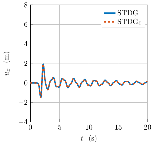

In Table 3 we collect the condition number of the system matrix, the number of GMRES iterations and the execution time for the STDG0 and STDG methods applied on a single time integration step, computed by using Domain A and Domain B, respectively. From the results we can observe that the proposed STDG method outperforms the STDG0 one, in terms of condition number and GMRES iteration counts for the solution of the corresponding linear system. Clearly, for small problems, when the storage of the system matrix and the use of a direct solvers is possible the STSG0 remains the most efficient solution.
| Dom. | Condition number | # GMRES it. | Execution time [s] | ||||
|---|---|---|---|---|---|---|---|
| STSG0 | STDG | STSG0 | STDG | STSG0 | STDG | ||
| A | 2 | ||||||
| A | 4 | ||||||
| B | 2 | ||||||
5.2.4 Layer over a half-space
In this experiment, we test the performance of the STDG method by considering a benchmark test case, cf. [22] for a real elastodynamics application, known in literature as layer over a half-space (LOH). We let be composed of two layers with different material properties, cf. Table 4. The domain is partitioned employing two conforming meshes of different granularity. The “fine” (resp. “coarse”) grid is composed of (resp. ) hexahedral elements, varying from size (resp. ), in the top layer, to (resp. ) in the bottom half-space, cf. Figure 9. On the top surface we impose a free surface condition, i.e. , whereas on the lateral and bottom surfacews we consider absorbing boundary conditions [54].

| Layer | Height | ||||
|---|---|---|---|---|---|
The seismic excitation is given by a double couple point source located at the center of the domain expressed by
| (38) |
where , is the scalar seismic moment, is the smoothness parameter, regulating the frequency content and amplitude of the source time function. The semi-analytical solution is available in [22] together with further details on the problem’s setup.
We employ the STDG method with different choices of polynomial degrees and time integration steps. In Figures 10-13 we show the velocity wave field computed at point along with the reference solution, in both the time and frequency domains, for the sets of parameters tested. We also report relative seismogram error
| (39) |
where is the number of samples of the seismogram, and are, respectively, the value of seismogram at sample and the corresponding reference value. In Table 5 we report the set of discretization parameters employed, together with some results obtaineds in terms of accuracy and computational efficiency.


| Grid | GMRES | Exec. Time | Tot. Exec. | Error | |||
|---|---|---|---|---|---|---|---|
| iter. | per iter. [s] | Time [s] | |||||
| Fine | |||||||
| Fine | |||||||
| Coarse | |||||||
| Coarse |
By employing the “fine” grid we obtain very good results both in terms of accuracy and efficiency. Indeed, the minimum relative error is less than with time polynomial degree , see Figure 10. Choosing , as in Figure 11, the error is larger (by a factor 40%) but the solution is still enough accurate. However, in terms of total Execution time, with the algorithm performs better than choosing , cf. Table 5, column 7. As shown in Figure 12, the “coarse” grid produces larger errors and worsen also the computational efficiency, since the number of GMRES iterations for a single time step increases. Doubling the integration time step , see Figure 13, causes an increase of the execution time for a single time step that partly compensate the decrease of total number of time steps. Consequently, the total execution time reduces but only by 12%. In addition, this choice causes some non-physical oscillations in the code part of the signal that contribute to increase the relative error. Indeed, we can conclude that for this test case, spatial discretization is the most crucial aspect. Refining the mesh produces a great decrease of the relative error and increases the overall efficiency of the method. Concerning time integration, it appears that the method performs well even with low order polynomial degrees both in terms of computational efficiency and of accuracy. The method achieves its goal of accurately solving this elastodynamics problem that counts between 119 (“coarse” grid) and 207 (“fine” grid) millions of unknowns. The good properties of the proposed STDG method is once again highlighted by the fact that all the presented results are achieved without any preconditioning of the linear system.
5.3 Seismic wave propagation in the Grenoble valley
In this last experiment, we apply the STDG method to a real geophysical study [19]. This application consists in the simulation of seismic wave propagation generated by an hypothetical earthquake of magnitude in the Grenoble valley, in the French Alps. The Y-shaped Grenoble valley, whose location is represented in Figure 14, is filled with late quaternary deposits, a much softer material than the one composing the surrounding mountains. We approximate the mechanical characteristics of the ground by employing three different material layers, whose properties are listed in Table 6. The alluvial basin layer contains soft sediments that compose the Grenoble’s valley and corresponds to the yellow portion of the domain in Figure 14. Then, the two bedrock layers approximate the stiff materials composing the surrounding Alps and the first crustal layer. The earthquake generation is simulated through a kinematic fault rapture along a plane whose location is represented in Figure 14.

| Layer | ||||
|---|---|---|---|---|
| Alluvial basin | 2140 + 0.125 | 300 + 19 | 1450 + 1.2 | 0.01 |
| Bedrock km | 2720 | 3200 | 5600 | 0 |
| Bedrock km | 2770 | 3430 | 5920 | 0 |
The computational domain is discretized with a fully unstructured hexahedral mesh represented in Figure 14. The mesh, composed of elements, is refined in the valley with a mesh size , while it is coarser in the bedrock layers reaching .


On the top surface we impose a free surface condition, i.e. , whereas on the lateral and bottom surface we consider absorbing boundary conditions [54]. We employ the STDG method with polynomial degrees for the space discretization and for the time integration, together with a time step . We focus on a set of monitor points whose location is represented in Figure 15. In Figure 16, we report the velocity field registered at these points compared with the ones obtained with a different code, namely SPECFEM [18]. The results are coherent with the different location of the points. Indeed, we observe highly perturbed waves in correspondence of the points that are located in the valley, i.e. in the alluvial material. This is caused by a refraction effect that arises when a wave moves into a soft material from a stiffer one. Moreover, the wave remains trapped inside the layer bouncing from the stiffer interfaces. The absence of this effect is evident from the monitors and that are located in the bedrock material. These typical behaviors are clearly visible also in Figure 17, where the magnitude of the ground velocity is represented for different time instants. Finally, concerning the computation efficiency of the scheme, we report that, with this choice of discretization parameters, we get a linear system with approximately millions of degrees of freedom that is solved in hours, employing parallel processes, on Marconi100 cluster located at CINECA (Italy).


6 Conclusions
In this work we have presented and analyzed a new time Discontinuous Galerkin method for the solution of a system of second-order differential equations. We have built an energy norm that naturally arose by the variational formulation of the problem, and that we have employed to prove well-posedness, stability and error bounds. Through a manipulation of the resulting linear system, we have reduced the computation cost of the solution phase and we have implemented and tested our method in the open-source software SPEED (http://speed.mox.polimi.it/). Finally, we have verified and validated the proposed numerical algorithm through some two- and three-dimensional benchmarks, as well as real geophysical applications.
7 Aknowledgements
This work was partially supported by ”National Group of Computing Science” (GNCS-INdAM). P.F. Antonietti has been supported by the PRIN research grant n. 201744KLJL funded by the Ministry of Education, Universities and Research (MIUR).
References
- [1] R. Abedi, B. Petracovici, and R. B. Haber. A space–time discontinuous Galerkin method for linearized elastodynamics with element-wise momentum balance. Computer Methods in Applied Mechanics and Engineering, 195:3247–3273, 2006.
- [2] R. A. Adams and J. J. F. Fournier. Sobolev spaces, volume 140 of Pure and Applied Mathematics. Elsevier, Amsterdam, second edition, 2003.
- [3] S. Adjerid and H. Temimi. A discontinuous Galerkin method for the wave equation. Computer Methods in Applied Mechanics and Engineering, 200(5):837 – 849, 2011.
- [4] P. F. Antonietti, B. Ayuso de Dios, I. Mazzieri, and A. Quarteroni. Stability analysis of discontinuous Galerkin approximations to the elastodynamics problem. Journal of Scientific Computing, 68:143–170, 2016.
- [5] P. F. Antonietti, N. Dal Santo, I. Mazzieri, and A. Quarteroni. A high-order discontinuous Galerkin approximation to ordinary differential equations with applications to elastodynamics. IMA Journal of Numerical Analysis, 38(4):1709–1734, 2018.
- [6] P. F. Antonietti, A. Ferroni, I. Mazzieri, R. Paolucci, A. Quarteroni, C. Smerzini, and M. Stupazzini. Numerical modeling of seismic waves by discontinuous spectral element methods. ESAIM: Proceedings and Surveys, 61:1–37, 2018.
- [7] P. F. Antonietti, A. Ferroni, I. Mazzieri, and A. Quarteroni. Dispersion-dissipation analysis of 3D continuous and discontinuous spectral element methods for the elastodynamics equation. Geophysics Journal International, 211(3):1554–1574, 2017.
- [8] P. F. Antonietti, A. Ferroni, I. Mazzieri, and A. Quarteroni. hp-version Discontinuous Galerkin approximations of the elastodynamics equation. Lecture Notes in Computational Science and Engineering, 119:3–19, 2017.
- [9] P. F. Antonietti and I. Mazzieri. High-order discontinuous Galerkin methods for the elastodynamics equation on polygonal and polyhedral meshes. Computer Methods in Applied Mechanics and Engineering, 342:414–437, 2018.
- [10] P. F. Antonietti, I. Mazzieri, and F. Migliorini. A space-time discontinuous Galerkin method for the elastic wave equation. Journal on Computational Physics, 419, 2020.
- [11] P. F. Antonietti, I. Mazzieri, A. Quarteroni, and F. Rapetti. Non-conforming high order approximations of the elastodynamics equation. Computer Methods in Applied Mechanics and Engineering, 209:212–238, 2012.
- [12] D. N. Arnold. An interior penalty finite element method with discontinuous elements. SIAM journal on numerical analysis, 19(4):742–760, 1982.
- [13] L. Banjai, E. H. Georgoulis, and O. Lijoka. A Trefftz polynomial space-time discontinuous Galerkin method for the second order wave equation. SIAM Journal of Numerical Analysis, 55:63–86, 2017.
- [14] P. Bansal, A. Moiola, I. Perugia, and C. Schwab. Space-time discontinuous Galerkin approximation of acoustic waves with point singularities. arXiv:2002.11575v2 [math.NA], 2020.
- [15] H. Barucq, H. Calandra, J. Diaz, and E. Shishenina. Space–time Trefftz-dg approximation for elasto-acoustics. Applicable Analysis, 99:747–760, 2018.
- [16] J. C. Butcher. Numerical Methods for Ordinary Differential Equations. Wiley, 2008.
- [17] A. Cangiani, E. H. Georgoulis, and P. Houston. -version discontinuous Galerkin methods on polygonal and polyhedral meshes. Mathematical Models and Methods in Applied Sciences, 24(10):2009–2041, 2014.
- [18] E. Chaljub, P. Moczo, S. Tsuno, P. Bard, J. Kristek, M. Käser, M. Stupazzini, and M. Kristeková. Quantitative comparison of four numerical predictions of 3d ground motion in the Grenoble valley, france. Bulletin of the Seismological Society of America, 100:1427–1455, 2010.
- [19] E. Chaljub, P. Moczo, S. Tsuno, P. Y. BArd, J. Kristek, M. Kaser, M. Stupazzini, and M. Kristekova. Quantitative comparison of four numerical predictions of 3d ground motion in the grenoble valley, france. Bulletin of the Seismological Society of America, 100:1427–1455, 2010.
- [20] B. Cockburn, G. E. Karniadakis, and C.-W. Shu, editors. Discontinuous Galerkin Methods. Theory, computation and applications. Lecture Notes in Computational Science and Engineering (Book 11). Springer, Berlin, 2000.
- [21] F. Collino, T. Fouquet, and P. Joly. A conservative space-time mesh refinement method for the 1-d wave equation. part i: Construction. Numerische Mathematik, (95):197 – 221, 2003.
- [22] S. M. Day and C. R. Bradley. Memory-efficient simulation of anelastic wave propagation. Bulletin of the Seismological Society of America, 19(3):520–531, 2001.
- [23] S. Delcourte and N. Glinsky. Analysis of a high-order space and time discontinuous Galerkin method for elastodynamic equations. application to 3d wave propagation. ESAIM: Mathematical Modelling and Numerical Analysis, 49(4):1085–1126, 2015.
- [24] M. Delfour, W. Hager, and F. Trochu. Discontinuous Galerkin methods for ordinary differential equations. Mathematics of Computation, 36(154):455–473, 1981.
- [25] D. A. Di Pietro and A. Ern. Mathematical aspects of Discontinuous Galerkin methods. Springer, 2011.
- [26] J. Diaz and M. J. Grote. Energy conserving explicit local time stepping for second-order wave equations. SIAM Journal of Scientific Computing, (31):1985 – 2014, 2009.
- [27] W. Dörfler, S. Findeisen, and C. Wieners. Space-time discontinuous Galerkin discretizations for linear first-order hyperbolic evolution systems. Computer Methods in Applied Mathematics, 16:409–428, 2016.
- [28] M. Dumbser, M. Käser, and E. Toro. An arbitrary high order discontinuous Galerkin method for elastic waves on unstructured meshes v: Local time stepping and -adaptivity. Geophys. J. Int., 171(2):695–717, 2007.
- [29] J. Ernesti and C. Wieners. Space-time discontinuous Petrov–Galerkin methods for linear wave equations in heterogeneous media. Computational Methods in Applied Mathematics, 19:465–481, 2019.
- [30] D. A. French. A space-time finite element method for the wave equation. Computer Methods in Applied Mechanics and Engineering, 107(1):145 – 157, 1993.
- [31] J. Gopalakrishnan, J. Schöberl, and C. Wintersteiger. Mapped tent pitching schemes for hyperbolic systems. Computational Methods in Science and Engineering, 39:B1043–B1063, 2017.
- [32] M. Grote, A. Schneebeli, and D. Schötzau. Discontinuous Galerkin finite element method for the wave equation. SIAM Journal on Numerical Analysis, 44(6):2408–2431, 2006.
- [33] M. J. Grote and T. Mitkova. High-order explicit local time-stepping methods for damped wave equations. Journal of Computational and Applied Mathematics, (239):270 – 289, 2013.
- [34] D. He and L. L. Thompson. Adaptive space–time finite element methods for the wave equation on unbounded domains. Computer Methods in Applied Mechanics and Engineering, 194:1947–2000, 2005.
- [35] J. S. Hesthaven and T. Warburton. Nodal Discontinuous Galerkin Methods: Algorithms, Analysis, and Applications. Springer Publishing Company, Incorporated, 1st edition, 2007.
- [36] P. Houston, C. Schwab, and E. Suli. Stabilized -finite element methods for first-order hyperbolic problems. SIAM Journal on Numerical Analysis, 37(5):1618–1643, 2000.
- [37] T. Hughes and G. Hulbert. Space-time finite element methods for elastodynamics: formulation and error estimates. Computer Methods in Applied Mechanics and Engineering, 66:339–363, 1988.
- [38] A. Idesman. Solution of linear elastodynamics problems with space–time finite elements on structured and unstructured meshes. Computer Methods in Applied Mechanics and Engineering, 196:1787–1815, 2007.
- [39] C. Johnson. Discontinuous Galerkin finite element methods for second order hyperbolic problems. Computer Methods in Applied Mechanics and Engineering, 107(1):117 – 129, 1993.
- [40] F. Kretzschmar, A. Moiola, I. Perugia, and S. M. Schenpp. A priori error analysis of space-time Trefftz discontinuous Galerkin methods for wave problems. IMA Journal of Numerical Analysis, 36:1599–1635, 2016.
- [41] A. Kroopnick. Bounded and -solutions to a second order nonlinear differential equation with a square integrable forcing term. International Journal of Mathematics and Mathematical Sciences, 22(3):569–571, 1999.
- [42] R. J. Le Veque. Finite Difference Methods for Ordinary and Partial Differential Equations. SIAM - Society for Industrial and Applied Mathematics, 2007.
- [43] P. Lesaint and P. Raviart. On a finite element method for solving the neutron transport equation. Publications des séminaires de mathématiques et informatique de Rennes, 1974.
- [44] I. Mazzieri, M. Stupazzini, R. Guidotti, and C. Smerzini. SPEED: Spectral Elements in Elastodynamics with Discontinuous Galerkin: a non-conforming approach for 3D multi-scale problems. International Journal for Numerical Methods in Engineering, 95(12):991–1010, 2013.
- [45] A. Moiola and I. Perugia. A space–time Trefftz discontinuous Galerkin method for the acoustic wave equation in first-order formulation. Numerische Mathematik, 138:389–435, 2018.
- [46] P. Monk and G. R. Richter. A discontinuous Galerkin method for linear symmetric hyperbolic systems in inhomogeneous media. Journal of Scientific Computing, 22:443–447, 2005.
- [47] I. Perugia, J. Schöberl, P. Stocker, and C. Wintersteiger. Tent pitching and Trefftz-dg method for the acoustic wave equation. Computers & Mathematics with Applications, 79:2987–3000, 2020.
- [48] A. Quarteroni, R. Sacco, and F. Saleri. Numerical Mathematics. Springer, 2007.
- [49] W. Reed and T. Hill. Triangular mesh methods for the neutron transport equation. Technical Report LA-UR-73-479, Los Alamos Scientific Laboratory, 1973.
- [50] B. Rivière. Discontinuous Galerkin methods for solving elliptic and parabolic equations: theory and implementation. Society for Industrial and Applied Mathematics, 2008.
- [51] B. Rivière and M. F. Wheeler. Discontinuous finite element methods for acoustic and elastic wave problems. Contemporary Mathematics, 329:271–282, 2003.
- [52] D. Schötzau and C. Schwab. Time discretization of parabolic problems by the -version of the discontinuous Galerkin finite element method. SIAM Journal on Numerical Analysis, 38(3):837–875, 2000.
- [53] D. Schötzau and T. P. Wihler. A posteriori error estimation for hp-version time-stepping methods for parabolic partial differential equations. Numerische Mathematik, 115:475–509, 2010.
- [54] R. Stacey. Improved transparent boundary formulations for the elastic-wave equation. Bulletin of the Seismological Society of America, 78(6):2089–2097, 1988.
- [55] O. Steinbach and M. Zank. A stabilized space–time finite element method for the wave equation. Advanced Finite Element Methods with Applications, pages 341–370, 2017.
- [56] T. Tezduyar, S. Sathe, R. Keedy, and K. Stein. Space–time finite element techniques for computation of fluid–structure interactions. Computer Methods in Applied Mechanics and Engineering, 195:2002–2027, 2006.
- [57] J. van der Vegt, C. Klaji, F. van der Bos, and H. van der Ven. Space-time discontinuous Galerkin method for the compressible navier-stokes equations on deforming meshes. European Conference on Computational Fluid Dynamics ECCOMAS CFD 2006, 2006.
- [58] T. Werder, K. Gerder, D. Schötzau, and C. Schwab. hp-discontinuous Galerkin time stepping for parabolic problems. Computer Methods in Applied Mechanics and Engineering, 190:6685–6708, 2001.
- [59] M. F. Wheeler. An elliptic collocation–finite element method with interior penalties. SIAM Journal on Numerical Analysis, 15(1):152–161, 1978.
- [60] L. C. Wilcox, G. Stadler, C. Burstedde, and O. Ghattas. A high-order discontinuous Galerkin method for wave propagation through coupled elastic-acoustic media. Journal of Computational Physics, 2010.
- [61] L. Yin, A. Acharya, N. Sobh, R. B. Haber, and D. A. Tortorelli. A space-time discontinuous Galerkin method for elastodynamic analysis. In B. Cockburn, G. E. Karniadakis, and C.-W. Shu, editors, Discontinuous Galerkin Methods, pages 459–464. Springer Berlin Heidelberg, 2000.