On Stretching, Bending, Shearing and Twisting of Actin Filaments I: Variational Models

In the Cosserat theory, a filament is mathematically described by a directed curve CARREGA 1981; Cohen and Desilva 1966. This consists of backbone curve $\bm{r}(\hat{s})\in{\mathbb{R}^{3}}$, where $\hat{s}\in[0,\hat{L}]$ is the reference arc-length coordinate, and an orthonormal triad of directors $\bm{D}(\hat{s})=\left(\bm{d}_{1}(\hat{s}),\ \bm{d}_{2}(\hat{s}),\ \bm{d}_{3}(\hat{s})\right)$. In our notation the caret hat symbol denotes a variable of the reference configuration. The column vectors $\bm{d}_{\alpha}(\hat{s})\in{\mathbb{R}^{3}}\!$, where $\alpha=1,2,3$ indexes the Cartesian components, specify the orientation of the rod’s cross-section at $\hat{s}$ such that $\bm{d}_{3}(\hat{s})$ is normal to the cross-section and $\bm{d}_{1}(\hat{s})$ and $\bm{d}_{2}(\hat{s})$ span the cross-section and define its twist about $\bm{d}_{3}(\hat{s})$. These vectors generally differ from the Frenet-Serret frame comprising the tangent, normal, and binormal vectors of $\bm{r}(\hat{s})$ Kreyszig 1968. We distinguish between the current configuration of the rod, described by $\bm{r}(\hat{s})$ and $\bm{D}(\hat{s})$, and the reference (un-deformed) configuration, described by a reference curve $\hat{\bm{r}}(\hat{s})$ and a reference triad $\widehat{\bm{D}}(\hat{s})=\left(\widehat{\bm{d}}_{1}(\hat{s}),\ \widehat{\bm{d}}_{2}(\hat{s}),\widehat{\bm{d}}_{3}(\hat{s})\right).$ Dilatation of the rod’s backbone length is captured by the scalar quantity $e(\hat{s})=\mbox{d}s/\mbox{d}\hat{s}$, which can be used to change coordinates from the reference arc-length coordinate $\hat{s}$ to the current arc-length coordinate $s$. In this paper we primarily use the reference coordinate system, although our formulation is equivalent to one using the current coordinate system. The proper orthogonal rotation $\bm{Q}(\hat{s})\in{\mathbb{R}^{3\times 3}}$ rotates the reference triad into the current one:

In what follows, we will assume $\widehat{\bm{D}}$ is independent of $\hat{s}$ to simplify notation. The quantities just introduced are illustrated in Figure 1.

From these quantities, six independent components of strain are defined Antman 2005; O’Reilly 2017. Three of these components are encoded in the pseudovector

where the ax operation returns the pseudovector associated¹¹ 1 The ax operation acts on a skew symmetric matrix $\bm{S}=\begin{pmatrix}0&-c&b\\ c&0&-a\\ -b&a&0\end{pmatrix}$ such that $\text{ax}(\bm{S})=\bm{v}=(a,b,c)^{T}$. Its inverse operation, skew, acts on $\bm{v}$ such that $\text{skew}(\bm{v})=\bm{S}$. These have the property that for any vector $\bm{x}$, $\bm{S}\bm{x}=\bm{v}\times\bm{x}$. with the skew-symmetric matrix $\bm{Q}^{T}\,\mbox{d}\bm{Q}\!\ /\ \mbox{d}\hat{s}$. The components of $\bm{\kappa}$ along the reference triad vectors, $\kappa_{\alpha}=\bm{\kappa}\cdot\widehat{\bm{d}}_{\alpha}$, measure the two bending strains, $\kappa_{1}$ and $\kappa_{2}$, and single twisting strain, $\kappa_{3}$, at each arc-length coordinate $\hat{s}$. Similarly, the components along $\widehat{\bm{d}}_{\alpha}$ of the vector

measure the two transverse shearing strains, $\sigma_{1}$ and $\sigma_{2}$, and the single stretching (extensional) strain, $\sigma_{3}$, completing the collection of six strain measures.

These strain components are used to define the elastic strain energy density $\varepsilon(\hat{s})$ of the rod’s configuration in the Cosserat theory Antman 2005; O’Reilly 2017. The filament’s total strain energy $E$ is obtained by integrating the density $\varepsilon(\hat{s})$ along the filament’s reference arc-length $\hat{L}$:

The most general quadratic expansion of the local energy density $\varepsilon(\hat{s})$ would include all 27 terms of the form $\kappa_{\alpha}\kappa_{\beta}$, $\kappa_{\alpha}\sigma_{\beta}$, and $\sigma_{\alpha}\sigma_{\beta}$, for $\alpha,\beta=1,2,3$, capturing mechanical couplings between all components of the strain De La Cruz et al. 2010; Yamaoka and Adachi 2010. However, the material symmetries of the rod can significantly reduce the number of terms needed to describe the energy. An actin filament can be approximately classified as a transversely hemitropic (i.e. spatially-averaged screw-symmetric) rod Healey 2002. It can be shown that such a rod has an energy density with the form Antman 2005

The coefficients $S_{\alpha,\beta}$, $B_{\alpha,\beta}$, and $C_{\alpha,\beta}$ can be viewed as elements of the parameter matrices $\bm{S}$, $\bm{B}$, and $\bm{C}$ appearing in the general quadratic expression of $\varepsilon$ O’Reilly 2017. They are geometric and material constants (rigidities) that parameterize the energy penalty of the rod in response to various deformations. The top row of terms in equation (5) captures the energy due to each mode of deformation individually. The bottom row, which would be zero for an isotropic material, captures couplings between these deformations. The twist-stretch coupling term proportional to $C_{3,3}$ is of particular interest in the case of actin, because it allows for chiral asymmetry in the filament’s torsional compliance Healey 2002; Smith and Healey 2008. We note that other mechanical coupling terms not included in equation (5), such as a twist-bend coupling term proportional to $(\kappa_{1}+\kappa_{2})\kappa_{3}$, can also play a role in the mechanics of short actin filaments for which spatial averaging is a poor approximation De La Cruz et al. 2010. Any such coupling terms, as well as higher order terms in the expansion of $\varepsilon$, could be easily accommodated by the methodology subsequently presented in this paper, but in our present applications we use equation (5) to describe chiral actin filaments.

To parameterize the model we need to specify the elements of $\bm{S}$, $\bm{B}$, and $\bm{C}$ which appear in equation (5). The diagonal elements of $\bm{S}$ and $\bm{B}$ can be expressed in terms of the material properties $E_{\text{mod}}$ and $G_{\text{mod}}$, representing the Young’s and shear moduli respectively, and the geometric properties $A$, $\bm{I}$, and $\alpha_{c}$, representing the cross-sectional area, second (polar) moment of inertia tensor, and a constant equal to $4/3$ for circular cross-sections. We give the details of the parameterization in the Supplementary material, Section B.1. The elements of $\bm{C}$ will be treated here as tunable parameters to study the effect of anisotropic mechanical compliance. We note that the elements of $\bm{C}$ are bounded by the requirement of energy positivity; for instance $|C_{3,3}|<\sqrt{S_{3,3}B_{3,3}}$ Healey 2002.

In one standard modeling approach, the energy $E$ is used to derive equations of motion which when numerically integrated propagate the rod’s configuration forward in time Spillmann and Teschner 2007; Bergou et al. 2008; Gazzola et al. 2018. Rather than numerically integrating a differential equation, which requires significant computational effort for large systems, the approach pursued in this paper is to efficiently find approximately equilibrated rod configurations under some external loads. In addition to the computational acceleration afforded by directly seeking minimized configurations, we are also motivated to pursue this approach because we aim to incorporate a filament model using the Cosserat theory into the simulation platform MEDYAN Popov et al. 2016. In MEDYAN, the system’s dynamics are propagated forward via short bursts of stochastic chemical activity over a reaction-diffusion compartment grid followed by periodic relaxation of the system’s mechanical energy; this allows for efficient simulations that include chemical reactions with spatially varying propensities Baras and Mansour 1996; Floyd et al. 2020. We note that this energy-minimization based approach to dynamics neglects the thermal diffusive motion of the filaments. The rationale behind this approach is that the ATP-consuming contributions to the system dynamics, coming from myosin motor steps and actin polymerization, significantly outweighs the contributions coming from diffusive motion of the filaments in these far-from-equilibrium systems Popov et al. 2016; Mizuno et al. 2007; MacKintosh and Schmidt 2010. As a result, neglecting thermal motion in MEDYAN simulations is not expected to significantly compromise the realism of the behaviors we are interested in, and this claim has been corroborated through several validations of MEDYAN predictions against experimental measurements Chandrasekaran et al. 2019; Komianos and Papoian 2018; Ni and Papoian 2019; Li et al. 2020; Ni and Papoian 2021; Floyd et al. 2021. Under some external loads, such as cross-linkers bound to the filament, the energy $E$ is variationally minimized for some continuous functions $\bm{r}^{\star}(\hat{s})$ and $\bm{Q}^{\star}(\hat{s})$, where the star denotes the energy-minimized configuration. This infinite-dimensional functional minimization problem is computationally burdensome, necessitating a more efficient scheme for scalable simulations.

The crucial approximation underlying our variational approach is similar in spirit to the Rayleigh-Ritz (or Ritz-Galerkin) method, in which an infinite-dimensional eigenvalue problem is converted to a finite-dimensional one via restriction to a finite-dimensional subspace of expansion coefficients for some chosen basis functions MacDonald 1933; Slaughter 1973. In our method, we assume that both $\bm{r}(\hat{s})$ and $\bm{Q}(\hat{s})$ are of a specified functional form having a discrete set of free parameters $\mathcal{K}$. We present two options for this: one in which $\bm{r}(\hat{s})$ and the Euler angles parameterizing $\bm{Q}(\hat{s})$ are spline functions of $\hat{s}$, and one in which $\bm{Q}(\hat{s})$ is the geodesic curve in $\mathrm{SO}(3)$ (the three-dimensional rotation group) on a segment of the filament while $\mbox{d}\bm{r}/\mbox{d}\hat{s}$ is parameterized using its components in the local $\bm{d}_{\alpha}(\hat{s})$ basis. The details of these functional forms are elaborated below. The strain energy density $\varepsilon(\hat{s};\mathcal{K})$ becomes a function of $\hat{s}$ and the parameters $\mathcal{K}$ through its definition in terms of the strain components, Equation 5. The key challenge in this variational approach is evaluating the integral in Equation 4 to express the total energy of the filament $E(\mathcal{K})$ as a function of the model parameters. Once this is done, equilibrated configurations of the the rod under some external loads, whose energy $E_{\text{ext}}(\mathcal{K})$ is also expressed in terms of the model parameters, are found by minimizing the total energy $E_{\text{tot}}(\mathcal{K})=E(\mathcal{K})+E_{\text{ext}}(\mathcal{K})$ with respect to the elements in $\mathcal{K}$. This yields the optimized parameters $\mathcal{K}^{\star}=\arg\min_{\mathcal{K}}E_{\text{tot}}(\mathcal{K})$, which determine the optimized configuration $\bm{r}^{\star}(\hat{s})=\bm{r}(\hat{s};\mathcal{K}^{\star})$ and $\bm{Q}^{\star}(\hat{s})=\bm{Q}(\hat{s};\mathcal{K}^{\star})$. We find that, using the spline representation for $\bm{r}(s;\mathcal{K})$ and the Euler angles of $\bm{Q}(\hat{s};\mathcal{K})$, it is necessary to expand $\varepsilon(\hat{s};\mathcal{K})$ around small values of the Euler angles for the integral in Equation 4 to be analytically solvable. Using the geodesic form for $\bm{Q}$, this approximation does not need to be made. We next give the details of these two variational methods.

Here we describe how to assign a functional form for the rod’s configuration, $\bm{r}(\hat{s})$ and $\bm{Q}(\hat{s})$, using spline functions. We refer to this approach as the “spline-based” model. Commonly used in the field of computer graphics, several spline functions are available such as B-splines, exponential splines, and Hermite splines, which may each have particular advantages depending on the application Shikin and Plis 1995; Prautzsch et al. 2002; Späth 1969; Neuman 1978. For the purpose of demonstrating this approach, we use here composite Bézier curves which are are fairly intuitive and easy to work with, but this method could be straightforwardly extended to use other splines. The reference arc-length $\hat{L}$ is discretized into $N_{\text{k}}-1$ segments whose ends are $N_{\text{k}}$ knot coordinates. The knot coordinates are particular values $\hat{s}_{i}$ of the reference arc-length, and the $i^{th}$ segment has a reference arc-length $\hat{L}_{i}=\hat{s}_{i+1}-\hat{s}_{i}$. This discretization is illustrated in Figure 1.

A composite Bézier curve $\bm{x}(\hat{s})$ is a piecewise function which passes through $N_{\text{k}}$ knot points $\bm{x}_{i}$, where $i=0,\ldots,N_{\text{k}}-1$. On the each segment $i$, $\bm{x}(\hat{s})$ is polynomial of order $d$ whose shape is controlled by the control points $\bm{x}_{i,j}$, where $j=0,\ldots,d-2$ and the double index indicates that $\bm{x}_{i,j}$ is a control point. Like $N_{\text{k}}$, the polynomial order $d$ is a hyperparameter controlling the complexity of the model. We will formulate the model for general values of these hyperparameters, but in our implementations we choose $d$ as $1$ or $2$ and $N_{\text{k}}$ such that an actin filament segment is $\sim 20-100\ \mbox{nm}$ long. In Figure 1, for instance, we have $N_{\text{k}}=6$ which is a typical value used. The full curve $\bm{x}(\hat{s})$ consists of $N_{\text{k}}-1$ segments $\bm{x}_{i}(\hat{s})$, $i=0,\ldots,N_{\text{k}}-2$, such that $\bm{x}(\hat{s})=\bm{x}_{i}(\hat{s})$ if $\hat{s}_{i}\leq\hat{s}<\hat{s}_{i+1}$. Here the argument of $\bm{x}_{i}(\hat{s})$ indicates that it is a function rather than a knot point. The segment curves $\bm{x}_{i}(\hat{s})$ are reparameterized using the segment variable $q(\hat{s};\hat{s}_{i},\hat{s}_{i+1})=(\hat{s}-\hat{s}_{i})/\hat{L}_{i}$ which ranges from $0$ to $1$ as $\hat{s}$ increases from $\hat{s}_{i}$ to $\hat{s}_{i+1}$. In terms of $q$, the segment curves are given by the formula

where the Bernstein polynomials are

If all knot and control points are free, then un-physical cusps can result in the composite curve at the knot points. To address this, smoothness up to degree $p$ can be enforced through derivative matching conditions

where $i=0,\ldots N_{k}-3,\ k=1,\ldots,p$ and $\bm{x}_{i}^{(k)}(\hat{s})$ denotes the $k^{\text{th}}$ derivative with respect to $\hat{s}$ of $\bm{x}_{i}(\hat{s})$. Choosing $p=d-1$ gives $3(d-1)(N_{\text{k}}-2)$ equations in $3(N_{\text{k}}+(N_{\text{k}}-1)(d-1))$ parameters, leaving $3(N_{\text{k}}+d-1)$ free. These free parameters can be taken to be the $N_{\text{k}}$ knot points $\bm{x}_{i}$ and the control points on the first segments, $\bm{x}_{0,j}$, $j=0,\ldots,d-2$. This choice of $p$ provides the greatest amount of smoothness while also allowing the number of free parameters to grow with $N_{\text{k}}$. One deficit of this parameterization is that specifying a position on the $i^{th}$ segments requires using parameters from segments $0$ to $i-1$, since the control points on the $i^{th}$ segment are determined from the smoothness constraints involving these previous parameters. However, for reasonably small values of $N_{\text{k}}$, up to $\sim 10$, this issue does not significantly impair model performance (we discuss the computational efficiency of these models in the Supplementary material, Section A.3).

A composite Bézier curve is used to represent both the backbone curve $\bm{r}(\hat{s})$ as well as the curve $\bm{\alpha}^{\text{Eu}}(\hat{s})$, containing the Euler angles parameterizing $\bm{Q}(\hat{s})$, as function of $\hat{s}$. The vector $\bm{\alpha}^{\text{Eu}}(\hat{s})=(\phi^{\text{Eu}}(\hat{s}),\ \theta^{\text{Eu}}(\hat{s}),\ \psi^{\text{Eu}}(\hat{s}))^{T}$ encodes here the 3-2-1 (yaw-pitch-roll) Euler angles of $\bm{Q}$, although other Euler angle conventions could also be used O’Reilly 2008. For this representation of $\bm{r}(\hat{s})$ and $\bm{Q}(\hat{s})$, the model parameters are $\mathcal{K}=\{\bm{r}_{0,0},\ldots,\bm{r}_{0,d_{r}-2},\bm{r}_{0},\ldots,\bm{r}_{N_{\text{k}}-1},\bm{\alpha}^{\text{Eu}}_{0,0},\ldots,\bm{\alpha}^{\text{Eu}}_{0,d_{\alpha}-2},\bm{\alpha}^{\text{Eu}}_{0},\ldots,\bm{\alpha}^{\text{Eu}}_{N_{\text{k}}-1}\}$ where $d_{r}$ and $d_{\alpha}$ are the orders of the composite Bézier curves for the backbone and Euler angles respectively. Using the above definitions of the strain components which enter into Equation 5, it is straightforward to write the strain energy density $\varepsilon(\hat{s};\mathcal{K})$ using these spline parameters. However, to find the integrated energy $E(\mathcal{K})$, it is necessary due to the intractability of analytically integrating $\varepsilon(\hat{s};\mathcal{K})$ to make a small-angle approximation to $\bm{Q}(\bm{\alpha}^{\text{Eu}})\approx\bm{Q}_{\text{approx.}}(\bm{\alpha}^{\text{Eu}};m)$. The order $m$ of the small-angle expansion is an additional hyperparameter of the model. Using $\bm{Q}_{\text{approx.}}$ in place of $\bm{Q}$ in the definition of the strain components, the approximate strain energy density $\varepsilon_{\text{approx.}}(\hat{s};\mathcal{K})$ becomes a polynomial in $\hat{s}$, that is

which may therefore be easily integrated to give the approximate energy of the filament $E_{\text{approx.}}(\mathcal{K})$. We implemented a routine to calculate $E_{\text{approx.}}(\mathcal{K})$ using the computer algebra system Mathematica Inc. 2020. The details of this calculation are tedious (though straightforward) and do not provide additional insight, so we do not present them here. They can be found in the accompanying Mathematica notebooks.

As discussed in Section 3, the small-angle approximation used to obtain an analytical expression for the integral of the energy density in the spline-based model can lead to biased filament configurations that are highly inaccurate when the deformations are large. To address this issue, we next present a so-called “geodesic” model which avoids making the small-angle approximation and produces approximately correct filament configurations even for large deformations.

In the geodesic model, we adopt the axis-angle parameterization for the rotation tensor $\bm{Q}$, rather than the Euler angle parameterization used above. In the axis-angle parameterization $\bm{Q}(\bm{u},\theta)$ represents a rotation about the unit vector $\bm{u}$ by the angle $\theta$. The Rodrigues formula expresses the tensor in terms of $\bm{u}$ and $\theta$ as

where $\bm{E}$ is the $3\times 3$ identity matrix, the skew operation returns the skew-symmetric matrix matrix associated with the unit vector $\bm{u}$ (and is the inverse of the ax operation), and $\otimes$ denotes the outer (dyadic) product O’Reilly 2017. $\bm{Q}(\bm{u},\theta)$ can also be represented using matrix exponentiation as

This representation makes evident the connection between the orthogonal tensor $\bm{Q}$, a member of the Lie group $\mathrm{SO}(3)$, and the skew-symmetric tensor $\text{skew}(\theta\bm{u})$, a member of the associated Lie algebra $\mathfrak{so}(3)$ Jeevanjee 2011. The transpose $\bm{Q}^{T}(\bm{u},\theta)$ can be obtained as $\bm{Q}^{T}(\bm{u},\theta)=\bm{Q}(\bm{u},-\theta)$.

We again use $N_{\text{k}}$ knot coordinates to discretize the filament into $N_{\text{k}}-1$ segments. At every knot coordinate $\hat{s}_{i}$ a rotation tensor $\bm{Q}_{i}$ is parameterized with free model parameters $\bm{u}^{\text{Ax}}_{i}$ and $\theta^{\text{Ax}}_{i}$. To enforce normalization, we represent $\bm{u}^{\text{Ax}}_{i}$ in polar coordinates using the polar and azimuthal angles, $\beta^{\text{Ax}}_{i}$ and $\gamma^{\text{Ax}}_{i}$ respectively. Thus the collection of angles $\theta^{\text{Ax}}_{i},\ \beta^{\text{Ax}}_{i}$, and $\gamma^{\text{Ax}}_{i}$ parameterize $\bm{Q}_{i}$ at $\hat{s}_{i}$. On the $i^{th}$ segment (where $\hat{s}_{i}\leq\hat{s}<\hat{s}_{i+1}$), the rotation tensor $\bm{Q}_{i}(q)$ is taken to be the geodesic curve on the manifold $\mathrm{SO}(3)$ which connects the two tensors $\bm{Q}_{i}$ and $\bm{Q}_{i+1}$, where $q(\hat{s};\hat{s}_{i},\hat{s}_{i+1})=(\hat{s}-\hat{s}_{i})/\hat{L}_{i}$ is the local segment variable as in the spline-based model. The geodesic curve depends on the metric $D$ used to define distances in $\mathrm{SO}(3)$, and we use the metric

where $\theta_{A,B}$ is the angle in the axis-angle parameterization of the tensor $\bm{Q}_{B}\bm{Q}_{A}^{T}$ rotating $\bm{Q}_{A}$ to $\bm{Q}_{B}$ Huynh 2009. It can be shown that the geodesic curve $\bm{Q}_{i}(q)$ connecting $\bm{Q}_{i}$ and $\bm{Q}_{i+1}$ using this metric is

where $\ln$ is the matrix logarithm Park 1995; Park and Ravani 1997. As described in the Supplementary material, Section B.2 this curve can then be expressed in terms of the free model parameters $\theta^{\text{Ax}}_{i},\ \beta^{\text{Ax}}_{i},\ \gamma^{\text{Ax}}_{i},\ \theta^{\text{Ax}}_{i+1},\ \beta^{\text{Ax}}_{i+1}$, and $\gamma^{\text{Ax}}_{i+1}$. The global tensor curve $\bm{Q}(\hat{s})$ is given piecewise by $\bm{Q}_{i}(\hat{s})$ on the $N_{\text{k}}-1$ segments.

To represent the backbone curve $\bm{r}(\hat{s})$ in the geodesic model, we write its derivative with respect to $\hat{s}$ in the local director triad basis $\bm{d}_{\alpha}$:

where summation over repeated indices is implied. Here we treat the components $\zeta_{\alpha}(\hat{s})$ as constants on each segment, i.e. $\zeta_{\alpha}(\hat{s})=\zeta_{i,\alpha}$ for $\hat{s}_{i}\leq\hat{s}<\hat{s}_{i+1}$, although this assumption could be relaxed. The piecewise constant components $\zeta_{i,\alpha}$ are additional free model parameters. We refer to the model where $\zeta_{i,\alpha}$ are all independent as the “geodesic Cosserat” (GC) model. We can also optionally set $\zeta_{i,1}=\zeta_{i,2}=0$ on all segments, implying that $\mbox{d}\bm{r}/\mbox{d}\hat{s}$ is everywhere parallel to $\bm{d}_{3}(\hat{s})$ such that there is zero shear on the filament. The filament is still extensible, since $\zeta_{i,3}\neq 0$, so this model is referred to as the “geodesic extensible Kirchoff” (GEK) model. To obtain the backbone curve $\bm{r}(\hat{s})$, we integrate $\mbox{d}\bm{r}/\mbox{d}\hat{s}$ from the minus-end position of the filament $\bm{r}_{0}=\bm{r}(\hat{s}=0)$, as shown in Equation 29 in the Supplementary material, Section B.2. The initial point $\bm{r}_{0}$ is the final free parameter in the GC and GEK models. We note that the filament energy $E(\mathcal{K})$ will not depend on $\bm{r}_{0}$ due to translation invariance, but external potentials $E_{\text{ext}}(\mathcal{K})$ such as cross-linkers bound to the filament will depend on $\bm{r}_{0}$. For the GC model, there are $6N_{\text{k}}$ elements in $\mathcal{K}$, while for the GEK model there $4N_{\text{k}}+2$.

A significant benefit of the geodesic parameterization of $\bm{r}(\hat{s})$ and $\bm{Q}(\hat{s})$ is that it allows the energy density to be analytically integrated along the length of the filament to give an exact expression for the total filament energy $E(\mathcal{K})$. We describe the derivation of this expression in the Supplementary material, Section B.3. As an intuitive picture, the geodesic curves used in this model can be thought of as representing a “linear” interpolation between rotation tensors in their natural mathematical space, and they are therefore expected to be a useful tool for parameterizing how several free rotation tensors are connected together.

For comparison, we describe here the original zero-width mechanical model used in the simulation platform MEDYAN Popov et al. 2016. This model has no allowed shearing or twisting, although excluded volume repulsion is included between filaments using a finite effective filament radius Floyd et al. 2021. The energy in this model does allow for stretching and bending. The filament is again discretized into $N_{\text{k}}$ knot coordinates and $N_{\text{k}}-1$ segments. Each segment is a straight line with a current length $L_{i}=s_{i+1}-s_{i}$ and a reference length $\hat{L}_{i}=\hat{s}_{i+1}-\hat{s}_{i}$. The stretching energy on each segment is a quadratic function of these lengths:

The segment acts like a spring with spring constant $S_{3,3}/\hat{L}_{i}$. At each internal knot coordinate there is a bending potential involving the angle $\theta^{\text{MED}}_{i,i+1}$ between the $i^{th}$ and $(i+1)^{th}$ segment:

where $i=1,\ldots,N_{\text{k}}-2$. We show in the Supplementary material, Section B.3 that this expression for the bending energy can be obtained as a special case of the GC model bending energy. In the MEDYAN model, the knot points $\bm{r}_{i}$ are the only free parameters, and the backbone curve $\bm{r}(\hat{s})$ is a linear interpolation between these points. There are thus $3N_{\text{k}}$ elements in $\mathcal{K}$ for this model.

We also briefly describe for comparison the dynamical model of a filament developed by Gazzola et al. in Ref. 35. Rather than directly seeking equilibrated configurations of the filament, the dynamical approach propagates the filament’s configuration forward in time using discretized equations of motion based on the forces and torques in the filament. Propagating the configuration forward for long times with dissipation will cause the filament to converge to its equilibrated configuration under some external loads. The filament in this model is discretized into $N_{\text{n}}-1$ linear segments which, when $N_{\text{n}}$ is large, allows for a good approximation to any arbitrary filament backbone configuration. In our usage here, we take $N_{\text{n}}\gg N_{\text{k}}$, so there are far fewer degrees of freedom in the variational models than in the dynamical model. The backbone $\bm{r}_{i}(t)$ is specified at each of the $N_{\text{n}}$ coordinates, and the rotation tensor $\bm{Q}_{i}(t)$ is specified on each of the $N_{\text{n}}-1$ segments. These quantities are updated in discrete time steps $\delta t$ using a second-order velocity Verlet integrator scheme. The equations of motion correspond to an isotropic energy function given by the top row of terms in Equation 5. For fine spatial and temporal discretization this model has been shown to be very expressive, capturing a range of realistic filament behaviors, and we use it in this paper as the “ground truth” to which our computationally accelerated variational models can be compared to assess their accuracy. We refer the reader to Ref. 35 for details of this model, and to the follow-up paper, Ref. 68, in which extensions to this dynamical model are developed to treat multiple spatial scales simultaneously.

In one-dimensional filament models like the original MEDYAN model, external loads such as bound cross-linkers on the filament are attached directly to the filament backbone. In the new models presented above, the filament has a finite width and external loads may attach to the surface of the filament, exerting shearing and twisting forces. This introduces an extra degree of freedom at the attached arc-length coordinate $\hat{s}^{\text{b}}$ corresponding to the position on the perimeter of the filament’s cross-section at $\hat{s}^{\text{b}}$ to which the load is attached. This cross-section is spanned by the vectors $\bm{d}_{1}(\hat{s}^{\text{b}})$ and $\bm{d}_{2}(\hat{s}^{\text{b}})$, and the one-dimensional position on the perimeter of the cross-section can be parameterized by the polar angle $\phi^{\text{b}}$ with respect to the local $\bm{d}_{1}(\hat{s}^{\text{b}})$ axis. For a circular cross section, the position of the attached load is given by

where $R$ is the filament radius. This position therefore couples not just to the backbone $\bm{r}(\hat{s}^{\text{b}})$ but also to the local rotation tensor $\bm{Q}(\hat{s}^{\text{b}})$ through $\bm{d}_{\alpha}(\hat{s})=\bm{Q}(\hat{s})\widehat{\bm{d}}_{\alpha}$. This binding of an attached linker to the local perimeter of the filament cross-section is illustrated in Figure 2.

By allowing for cross-linkers to bind to the surface of a filament rather than its backbone, an extra degree of freedom $\phi^{\text{b}}$ is introduced. We note that during a simulated binding event, this degree of freedom could be chosen in several ways, which we describe in the Supplementary material. For example, to provide additional biological realism a modeller could fix $\phi^{\text{b}}$ for the possible binding sites to lie along a helix which wraps around the filament. In this way, the helical microstructure of actin could be encoded into the available binding sites.

To assess the accuracy of the spline-based and geodesic models introduced above, we compare their equilibrated configurations to the steady state configuration of the finely-discretized dynamical model with dissipation. Five models are compared against the dynamical model: the Bézier spline-based model with a first order small-angle expansion (“B, $m=1$”), the Bézier spline-based model with a second order small-angle expansion (“B, $m=2$”), the geodesic extensible Kirchoff model (GEK), the geodesic Cosserat model (GC), and the original MEDYAN model. To quantify the difference between the equilibrated configurations, we use two similarity measures. The first, $C_{r}$, measures the root-mean-squared distance between the backbone curves of two filaments $A$ and $B$:

where $\lvert\lvert\cdot\rvert\rvert$ denotes the vector norm. The second similarity measure, $C_{d}$, is introduced to measure the average difference in the vectors $\bm{d}_{3}^{A}(\hat{s})$ and $\bm{d}_{3}^{B}(\hat{s})$ along the reference arc-length:

Both $C_{r}$ and $C_{d}$ are evaluated numerically using a large number of sample points.

Three test cases, labeled (A), (B) and (C) in Figure 3 were used to assess the models’ accuracy. The deformation in each test case is in a 2D plane so that the configurations can be easily visualized. In test case (A), a $500$ nm-long filament is pulled by four springs in opposing directions, while in test cases (B) and (C), a $100$ nm long filament is pulled by three springs. Test cases (B) and (C) are distinguished by the strength of the pulling such that the springs in test case (C) are much more stretched than those in (B), causing a greater filament deformation. The filaments in each test case are modeleled as isotropic (with the coupling matrix elements $C_{\alpha,\beta}$ in Equation 5 set to zero), and the springs attach directly to the filament backbone. This is done to allow comparison with the original MEDYAN model and the dynamical model implementations, which do not currently support anisotropic filaments or surface-bound cross-linkers. The details of the set up for these test cases are described in the Supplementary material, Section A.2.

For the three test cases, we generally observed that the closest agreement with the dynamical solution was obtained by the geodesic models, however for the small deformations in test case (B) all models agree well with each other (see Table 1). This indicates the sufficiency of the small-angle approximation for small applied loads. For large loads, the spline-based models have systematically smaller deformations than the geodesic and dynamical models, which is a major shortcoming. The original MEDYAN model does not exhibit this systematic error though it is less precise due to its linear segment shapes. The difference between the GEK and GC models is negligible for all test cases, resulting from the high shearing modulus of actin; the extra degrees of freedom in the GC model should still be useful for modeling other types of filaments. Both geodesic models agree very well with the dynamical solution, with only slight differences in shape even for large applied loads. Minimizing the geodesic models to obtain the equilibrated configurations takes on the order of seconds of computational time, however, whereas propagating the finely discretized dynamical model until it is equilibrated takes on the order of days. We display in the Supplementary material, Section A.4 the profile of shearing, extensional, bending, and twisting strain for the variational models along the length of the equilibrated filament for the third test case. We also show in the Supplementary material, Section A.3 the computational timing of the variational models along with their accuracy as $N_{\text{k}}$ is varied. Finally, we show in Table 2 the equilibrated filament and spring energies for each test case. We see that in each case the dynamical model achieves the smallest total energy of all models, which we might expect due to its comparative lack of restrictions on the filament configuration. However, the agreement in energy between the geodesic models and the dynamical model is excellent. Although in these test cases the difference between the GEK and GC models is small, we expect that in the context of real cytoskeletal networks, where molecular motors and branching molecules bind to the surfaces of filaments, the shearing degrees of freedom in the GC will be important. Such bound molecules can produce localized shearing forces which would not be resolved in the GEK model.

Here we apply the new variational models to explore the induced chirality of a bundle of cross-linked actin filaments. The intuition underlying this study is based on actin stress fibers, which are bundles comprising $\sim 7-20$ filaments under significant tensile stress that transmit cell-wide forces during processes like cell migration Fletcher and Mullins 2010; Chandrasekaran et al. 2019. The chiral coupling between axial stretching and filament twisting, captured by the $C_{3,3}$ parameter, opens the possibility that the filaments in a stress fiber also experience significant torsion under axial stress. We hypothesize that, due to the finite width of the actin filaments, this torsion will move the attached point of the bound cross-linker protein which will in turn pull on the other filament to which it’s bound. This will cause the peripheral filaments to tilt with respect to the central filament, such that the entire bundle structure acquires a helical pitch due to the applied tension, the twist-stretch coupling, and the bound cross-linkers.

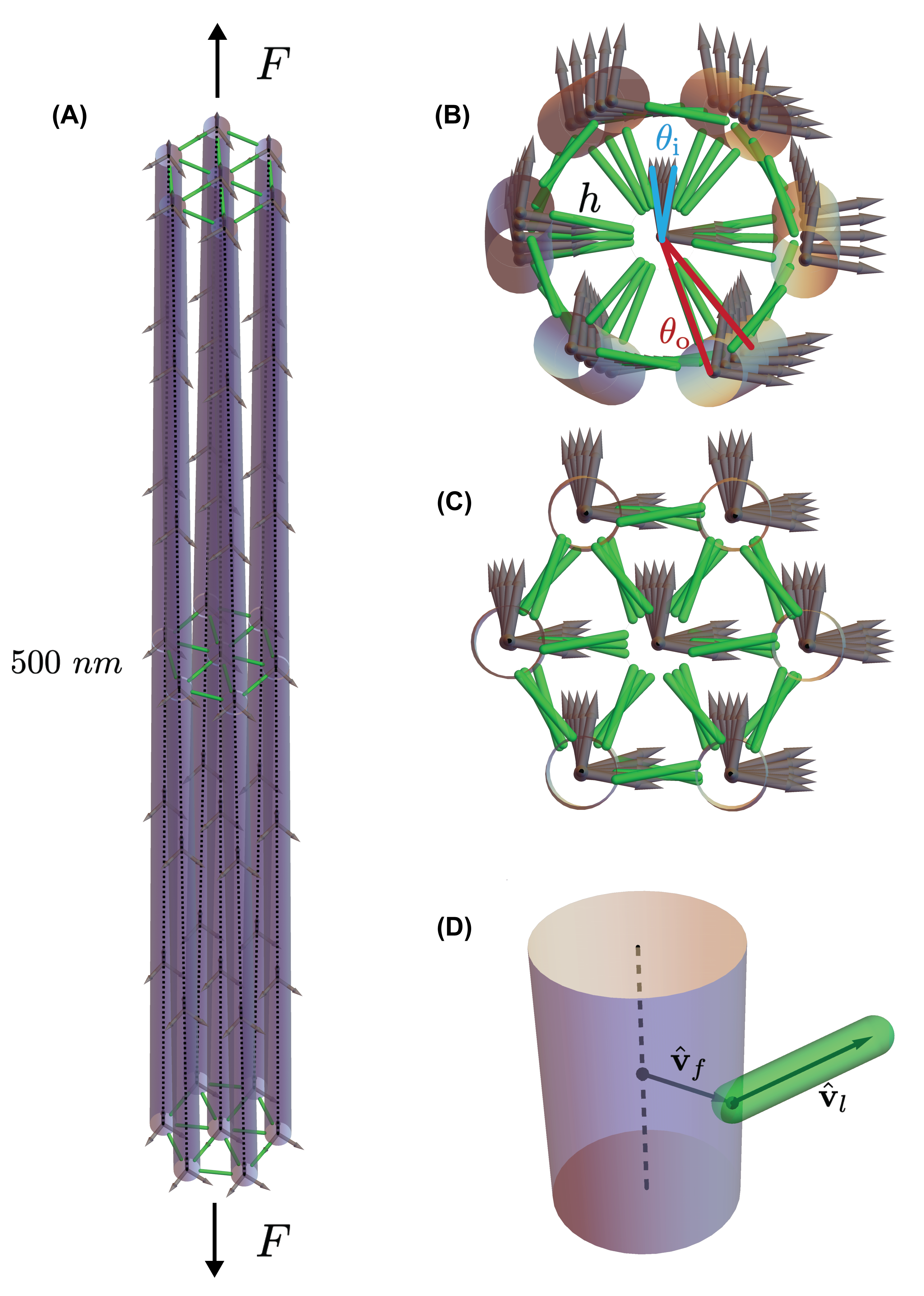
To explore this possible effect, we simulated $7$ filaments, each $500\ \mbox{nm}$ long and $7$ nm in diameter, in a bundle connected by $3$ sets of cross-linkers attached in a spoke and rim pattern, as visualized in Figures 4.A, B, and C. Each filament represented using the $\text{B},\ m=1$ model with $3$ knot points. Despite its less accurate performance under large applied loads (as shown in Figure 3), this model was observed to be consistent with other models tested for this study, and we use it here because it produced the cleanest trends due to its easily minimized energy function. The axial tension of a stress fiber was modeled by applying a constant $z$-direction force $F$ in opposite directions to both ends of every filament in the bundle. The attached cross-linkers have a stretching energy given by

where $l$ is the cross-linker’s instantaneous length and $h$ is its rest length. With only this energy included, the peripheral filaments in the bundle tend to twist under tension and move inward toward the bundle center, allowing the lengths of the cross-linkers to achieve their rest lengths without causing the filaments to tilt (see Figure 4.C). Certain actin binding proteins such as Arp2/3 are known to form relatively rigid angles with respect to the actin filament Goley and Welch 2006. To account for this possibility, we also include a steric interaction which penalizes cross-linker orientations deviating from the local surface normal of the filament, with an energy given by

where the unit vector $\hat{\bm{v}}_{f}$ denotes the local surface normal and $\hat{\bm{v}}_{l}$ denotes the unit vector pointing along the cross-linker’s length from the local attachment point (see Figure 4.D. for an illustration of these vectors). This steric geometric penalty has the effect that the bundle is less compressible, such that filaments are less able to move toward the bundle center and will instead tend to tilt and rotate to satisfy the linker length penalty. The adjustable parameters of this set-up are $F$, $C_{3,3}$, $\varepsilon_{\text{steric}}$, $k_{\text{linker}}$, and $h$. We independently varied these parameters one at a time, holding the other parameters at their default values of $F=100\ \mbox{pN}$, $C_{3,3}=10^{5}\ \mbox{pN}\ \mbox{nm}$, $\varepsilon_{\text{steric}}=500\ \mbox{pN}\ \mbox{nm}$, $k_{\text{linker}}=10\ \mbox{pN}/\mbox{nm}$, and $h=8\ \mbox{nm}$.

We distinguish between the inner and the outer rotation of the bundle under tension. The inner rotation $\theta_{\text{i}}$ is the angle through with the central filament is twisted from its minus end to its plus end, and we define $\gamma_{\text{i}}=|\theta_{\text{i}}|/\hat{L}$ as the rotation per unit length. To measure the tilting of the peripheral filaments around the central filament, we define the outer rotation $\theta_{\text{o}}$ as a function of the distance $\delta r$ by which a given outer filament’s endpoints are separated from each other when projected to the $xy$-plane. If the distance from a peripheral filament’s endpoint to the central filament’s endpoint (i.e. the radius of the bundle) is $a$, then the outer rotation angle is defined as $\theta_{\text{o}}=\arccos\left(1-(\delta r)^{2}/2a^{2}\right)$, given per unit length as $\gamma_{\text{o}}=|\theta_{\text{o}}|/\hat{L}$ (see Figure 4.B for an illustration of these angles). The inner rotation $|\theta_{\text{i}}|$ will always be greater than or equal to $|\theta_{\text{o}}|$, and if the cross-linkers perfectly transmit the rotation of the filaments into the tilting of the outer ring, then $|\theta_{\text{i}}|=|\theta_{\text{o}}|$.

Several notable trends are observed in this study, displayed in Figure 5. First, we find a transition from a linear dependence of both $\gamma_{\text{o}}$ and $\gamma_{\text{i}}$ on $F$ to sublinear dependence, at which point the outer and inner rotations also begin to separate from each other so that $\gamma_{\text{i}}>\gamma_{\text{o}}$ (Figure 5.A). This behavior is also symmetric about $F=0$, with compression inducing twisting in an approximately equal but opposite amount to stretching for small loads. These observations qualitatively agree with the intuition of linear response for small disturbances transitioning to nonlinear response for large disturbances. We also find a transition from linear to superlinear dependence on $C_{3,3}$ (Figure 5.D).

Second, we find a strong nonlinear dependence of $\gamma_{\text{o}}$ and $\gamma_{\text{i}}$ on $\varepsilon_{\text{steric}}$ resembling a second-order phase transition (Figure 5.B) Binney et al. 1992. Below an apparent threshold around $\varepsilon_{\text{steric}}\approx 0.1\ \mbox{pN}\ \mbox{nm}$ the applied force rotates the central filament by a fixed amount and the peripheral filaments rotate and move inward to satisfy the cross-linker length energy penalty. Above this threshold, and in a continuous manner, the steric penalty causes the filaments to tilt and bend rather than move inward to satisfy the cross-linker length penalty, causing $\gamma_{\text{o}}$ to increase and $\gamma_{\text{i}}$ to decrease. Above an upper threshold around $\varepsilon_{\text{steric}}\approx 100\ \mbox{pN}\ \mbox{nm}$ this trend saturates, and only small, though interestingly non-monotonic, changes are observed in $\gamma_{\text{i}}$ and $\gamma_{\text{o}}$ which now roughly coincide. Similar behavior is found for the dependence on $k_{\text{linker}}$, although the outer rotation below the lower transition threshold $\sim 0.01\ \mbox{pN}/\mbox{nm}$ is constant at a finite value, not zero, implying that the steric penalty alone can cause outer rotation of the bundle (Figure 5.E).

Third, we find that as the cross-linker resting length $h$ is increased, both $\gamma_{\text{i}}$ and $\gamma_{\text{o}}$ monotonically decrease, and $\gamma_{\text{i}}$ grows relative to $\gamma_{\text{o}}$ suggesting less effective transduction of inner rotation to outer rotation for large linker lengths (Figure 5.C). We also tested the effect of randomly placing the cross-linkers between the filaments rather than at the ends and midpoint of the filaments, controlling for the number of cross-linkers between each pair. For each value of $h$, we sampled 100 realizations of cross-linker positions with uniform probability along the filament lengths. We expected that the ordered (but statistically unlikely) arrangement of cross-linkers enhances the transduction of inner to outer rotation because the forces throughout the bundle are highly coordinated. The rare configuration with ordered cross-linkers is indeed more effective at causing outer rotation than the typical random configuration, as shown by the dotted lines in Figure 5.C which have larger $\gamma_{\text{i}}$ and smaller $\gamma_{\text{o}}$ for all $h$.

Finally, we tested how the mechanical coupling between twisting and stretching affected the force-extension curve of the bundle, shown in Figure 5.F. The equilibrated length $L$ of the central filament was measured as a function of the pulling force and divided by its initial value $\hat{L}=500\ \mbox{nm}$ to give the relative extension. We found that a non-zero $C_{3,3}$ allows for greater extension and greater compression for a given force $F$. For $C_{3,3}=0\ \mbox{pN}\ \mbox{nm}$ the force-extension curve is perfectly linear, while for $C_{3,3}\neq 0\ \mbox{pN}\ \mbox{nm}$ it smoothly interpolates between an asymptotically linear regime for $F\gg 0\ \mbox{pN}$ and a nonlinear crossing regime around the point $C_{3,3}=0\ \mbox{pN}\ \mbox{nm},\ F=0\ \mbox{pN}$.

As a final application, we implemented the GC model into MEDYAN Popov et al. 2016. This implementation consists of several new modelling choices, which we describe in detail in the Supplementary material. These new modelling choices have to do with allowing for chemical reactions, such as cross-linkers and molecular motors binding to filaments and filament polymerization and depolymerization reactions, using the new filament mechanical model presented in this paper. These additional chemical considerations, which allow the current mechanical model to be incorporated in a versatile active matter simulation platform, should significantly expand the model’s usefulness in studying cytoskeletal dynamics.

In Figure 6 we show a snapshot from a MEDYAN simulation, in which an actomyosin network comprising physiological concentrations of actin, myosin (non-muscle myosin IIA) and cross-linkers ($\alpha$-actinin) has undergone a network-wide contraction away from the simulation boundaries. This motor-driven contraction is in keeping with well-documented behavior of actomyosin networks at these concentrations Popov et al. 2016; Floyd et al. 2019; Linsmeier et al. 2016. The key point is that the network in Figure 6 has binding molecules attached to the surfaces of the actin filaments rather than their backbones, allowing for network-level shearing and twisting forces, filament rotational dynamics, and chiral phenomenon to be studied in silico. We report here only the feasibility of implementing the GC model into a network-level simulation platform like MEDYAN, rather than any trends observed using this implementation which we plan to explore in depth in future works.

References

- Fletcher and Mullins [2010] Fletcher, D. A.; Mullins, R. D. Cell mechanics and the cytoskeleton. Nature 2010, 463, 485–492.
- Howard et al. [2001] Howard, J., et al. Mechanics of motor proteins and the cytoskeleton. 2001,
- McCullagh et al. [2014] McCullagh, M.; Saunders, M. G.; Voth, G. A. Unraveling the mystery of ATP hydrolysis in actin filaments. Journal of the American Chemical Society 2014, 136, 13053–13058.
- Belmont et al. [1999] Belmont, L. D.; Orlova, A.; Drubin, D. G.; Egelman, E. H. A change in actin conformation associated with filament instability after Pi release. Proceedings of the National Academy of Sciences 1999, 96, 29–34.
- Mani et al. [2021] Mani, S.; Katkar, H. H.; Voth, G. A. Compressive and Tensile Deformations Alter ATP Hydrolysis and Phosphate Release Rates in Actin Filaments. Journal of Chemical Theory and Computation 2021, 17, 1900–1913.
- Mizuno et al. [2007] Mizuno, D.; Tardin, C.; Schmidt, C. F.; MacKintosh, F. C. Nonequilibrium mechanics of active cytoskeletal networks. Science 2007, 315, 370–373.
- Cordes et al. [2020] Cordes, A.; Witt, H.; Gallemí-Pérez, A.; Brückner, B.; Grimm, F.; Vache, M.; Oswald, T.; Bodenschatz, J.; Flormann, D.; Lautenschläger, F., et al. Prestress and area compressibility of actin cortices determine the viscoelastic response of living cells. Physical Review Letters 2020, 125, 068101.
- Gardel et al. [2004] Gardel, M.; Shin, J. H.; MacKintosh, F.; Mahadevan, L.; Matsudaira, P.; Weitz, D. A. Elastic behavior of cross-linked and bundled actin networks. Science 2004, 304, 1301–1305.
- Ajeti et al. [2019] Ajeti, V.; Tabatabai, A. P.; Fleszar, A. J.; Staddon, M. F.; Seara, D. S.; Suarez, C.; Yousafzai, M. S.; Bi, D.; Kovar, D. R.; Banerjee, S., et al. Wound healing coordinates actin architectures to regulate mechanical work. Nature physics 2019, 15, 696–705.
- Floyd et al. [2019] Floyd, C.; Papoian, G. A.; Jarzynski, C. Quantifying dissipation in actomyosin networks. Interface focus 2019, 9, 20180078.
- Yamaoka et al. [2012] Yamaoka, H.; Matsushita, S.; Shimada, Y.; Adachi, T. Multiscale modeling and mechanics of filamentous actin cytoskeleton. Biomechanics and modeling in mechanobiology 2012, 11, 291–302.
- Broedersz and MacKintosh [2014] Broedersz, C. P.; MacKintosh, F. C. Modeling semiflexible polymer networks. Reviews of Modern Physics 2014, 86, 995.
- Rubinstein et al. [2003] Rubinstein, M.; Colby, R. H., et al. Polymer physics; Oxford university press New York, 2003; Vol. 23.
- Freedman et al. [2017] Freedman, S. L.; Banerjee, S.; Hocky, G. M.; Dinner, A. R. A versatile framework for simulating the dynamic mechanical structure of cytoskeletal networks. Biophysical journal 2017, 113, 448–460.
- Nedelec and Foethke [2007] Nedelec, F.; Foethke, D. Collective Langevin dynamics of flexible cytoskeletal fibers. New Journal of Physics 2007, 9, 427.
- Kim et al. [2009] Kim, T.; Hwang, W.; Lee, H.; Kamm, R. D. Computational analysis of viscoelastic properties of crosslinked actin networks. PLoS Comput Biol 2009, 5, e1000439.
- Popov et al. [2016] Popov, K.; Komianos, J.; Papoian, G. A. MEDYAN: Mechanochemical simulations of contraction and polarity alignment in actomyosin networks. PLoS computational biology 2016, 12, e1004877.
- Floyd et al. [2021] Floyd, C.; Chandresekaran, A.; Ni, H.; Ni, Q.; Papoian, G. A. Segmental Lennard-Jones interactions for semi-flexible polymer networks. Molecular Physics 2021, e1910358.
- Tee et al. [2015] Tee, Y. H.; Shemesh, T.; Thiagarajan, V.; Hariadi, R. F.; Anderson, K. L.; Page, C.; Volkmann, N.; Hanein, D.; Sivaramakrishnan, S.; Kozlov, M. M., et al. Cellular chirality arising from the self-organization of the actin cytoskeleton. Nature cell biology 2015, 17, 445–457.
- Schaller et al. [2010] Schaller, V.; Weber, C.; Semmrich, C.; Frey, E.; Bausch, A. R. Polar patterns of driven filaments. Nature 2010, 467, 73–77.
- Fritzsche et al. [2017] Fritzsche, M.; Li, D.; Colin-York, H.; Chang, V.; Moeendarbary, E.; Felce, J.; Sezgin, E.; Charras, G.; Betzig, E.; Eggeling, C. Self-organizing actin patterns shape membrane architecture but not cell mechanics. Nature communications 2017, 8, 1–14.
- Egelman et al. [1982] Egelman, E.; Francis, N.; DeRosier, D. F-actin is a helix with a random variable twist. Nature 1982, 298, 131–135.
- Enrique and Gardel [2015] Enrique, M.; Gardel, M. L. Actin mechanics and fragmentation. Journal of Biological Chemistry 2015, 290, 17137–17144.
- Beausang et al. [2008] Beausang, J. F.; Schroeder 3rd, H. W.; Nelson, P. C.; Goldman, Y. E. Twirling of actin by myosins II and V observed via polarized TIRF in a modified gliding assay. Biophysical journal 2008, 95, 5820–5831.
- Vilfan [2009] Vilfan, A. Twirling motion of actin filaments in gliding assays with nonprocessive myosin motors. Biophysical journal 2009, 97, 1130–1137.
- Naganathan et al. [2014] Naganathan, S. R.; Fürthauer, S.; Nishikawa, M.; Jülicher, F.; Grill, S. W. Active torque generation by the actomyosin cell cortex drives left–right symmetry breaking. elife 2014, 3, e04165.
- Naganathan et al. [2016] Naganathan, S. R.; Middelkoop, T. C.; Fürthauer, S.; Grill, S. W. Actomyosin-driven left-right asymmetry: from molecular torques to chiral self organization. Current opinion in cell biology 2016, 38, 24–30.
- Ma and Berro [2018] Ma, R.; Berro, J. Structural organization and energy storage in crosslinked actin assemblies. PLoS computational biology 2018, 14, e1006150.
- De La Cruz et al. [2010] De La Cruz, E. M.; Roland, J.; McCullough, B. R.; Blanchoin, L.; Martiel, J. L. Origin of twist-bend coupling in actin filaments. Biophysical Journal 2010, 99, 1852–1860.
- Yamaoka and Adachi [2010] Yamaoka, H.; Adachi, T. Coupling between axial stretch and bending/twisting deformation of actin filaments caused by a mismatched centroid from the center axis. International Journal of Mechanical Sciences 2010, 52, 329–333.
- Cyron et al. [2013] Cyron, C. J.; Müller, K. W.; Bausch, A. R.; Wall, W. A. Micromechanical simulations of biopolymer networks with finite elements. Journal of Computational Physics 2013, 244, 236–251.
- Müller et al. [2015] Müller, K. W.; Meier, C.; Wall, W. A. Resolution of sub-element length scales in Brownian dynamics simulations of biopolymer networks with geometrically exact beam finite elements. Journal of Computational Physics 2015, 303, 185–202.
- CARREGA [1981] CARREGA, J.-C. Théorie des corps; A. Hermann et fils, 1981.
- Rubin [2000] Rubin, M. Cosserat Theories: Shells, Rods and Points; Springer, 2000.
- Gazzola et al. [2018] Gazzola, M.; Dudte, L.; McCormick, A.; Mahadevan, L. Forward and inverse problems in the mechanics of soft filaments. Royal Society open science 2018, 5, 171628.
- Antman [2005] Antman, S. Nonlinear Problems of Elasticity, volume 107 of Applied Mathematical Sciences, 2nd edn Springer. New York 2005, 1.
- O’Reilly [2017] O’Reilly, O. M. Modeling Nonlinear Problems in the Mechanics of Strings and Rods; Springer, 2017.
- Kirchhoff [1859] Kirchhoff, G. Ueber das Gleichgewicht und die Bewegung eines unendlich dünnen elastischen Stabes. Journal für die reine und angewandte Mathematik 1859, 1859, 285–313.
- Dill [1992] Dill, E. H. Kirchhoff’s theory of rods. Archive for History of Exact Sciences 1992, 44, 1–23.
- Bergou et al. [2008] Bergou, M.; Wardetzky, M.; Robinson, S.; Audoly, B.; Grinspun, B. ACM SIGGRAPH ASIA 2008 Courses, SIGGRAPH Asia’08; 2008; pp 1–12.
- Zhang et al. [2019] Zhang, X.; Chan, F. K.; Parthasarathy, T.; Gazzola, M. Modeling and simulation of complex dynamic musculoskeletal architectures. Nature communications 2019, 10, 1–12.
- Cohen and Desilva [1966] Cohen, H.; Desilva, C. N. Nonlinear theory of elastic directed surfaces. Journal of Mathematical Physics 1966, 7, 960–966.
- Kreyszig [1968] Kreyszig, E. Introduction to differential geometry and Riemannian geometry; University of Toronto Press, 1968.
- Healey [2002] Healey, T. Material symmetry and chirality in nonlinearly elastic rods. Mathematics and Mechanics of Solids 2002, 7, 405–420.
- Smith and Healey [2008] Smith, M. L.; Healey, T. J. Predicting the onset of DNA supercoiling using a non-linear hemitropic elastic rod. International Journal of Non-Linear Mechanics 2008, 43, 1020–1028.
- Spillmann and Teschner [2007] Spillmann, J.; Teschner, M. CORDE: Cosserat rod elements for the dynamic simulation of one-dimensional elastic objects. Symposium on Computer Animation 2007 - ACM SIGGRAPH / Eurographics Symposium Proceedings, SCA 2007. 2007; pp 63–72.
- Baras and Mansour [1996] Baras, F.; Mansour, M. M. Reaction-diffusion master equation: A comparison with microscopic simulations. Physical Review E 1996, 54, 6139.
- Floyd et al. [2020] Floyd, C.; Papoian, G. A.; Jarzynski, C. Gibbs free energy change of a discrete chemical reaction event. The Journal of chemical physics 2020, 152, 084116.
- MacKintosh and Schmidt [2010] MacKintosh, F. C.; Schmidt, C. F. Active cellular materials. Current opinion in cell biology 2010, 22, 29–35.
- Chandrasekaran et al. [2019] Chandrasekaran, A.; Upadhyaya, A.; Papoian, G. A. Remarkable structural transformations of actin bundles are driven by their initial polarity, motor activity, crosslinking, and filament treadmilling. PLoS computational biology 2019, 15, e1007156.
- Komianos and Papoian [2018] Komianos, J. E.; Papoian, G. A. Stochastic ratcheting on a funneled energy landscape is necessary for highly efficient contractility of actomyosin force dipoles. Physical Review X 2018, 8, 021006.
- Ni and Papoian [2019] Ni, Q.; Papoian, G. A. Turnover versus treadmilling in actin network assembly and remodeling. Cytoskeleton 2019,
- Li et al. [2020] Li, X.; Ni, Q.; He, X.; Kong, J.; Lim, S.-M.; Papoian, G. A.; Trzeciakowski, J. P.; Trache, A.; Jiang, Y. Tensile Force Induced Cytoskeletal Reorganization: Mechanics Before Chemistry. BioRxiv 2020,
- Ni and Papoian [2021] Ni, H.; Papoian, G. A. Membrane-medyan: Simulating deformable vesicles containing complex cytoskeletal networks. bioRxiv 2021,
- Floyd et al. [2021] Floyd, C.; Levine, H.; Jarzynski, C.; Papoian, G. A. Understanding cytoskeletal avalanches using mechanical stability analysis. Proceedings of the National Academy of Sciences 2021, 118.
- MacDonald [1933] MacDonald, J. K. Successive approximations by the Rayleigh-Ritz variation method. Physical Review 1933, 43, 830–833.
- Slaughter [1973] Slaughter, W. S. North-Holland Series in Applied Mathematics and Mechanics; Springer Science & Business Media, 1973; Vol. 16; pp 46–78.
- Shikin and Plis [1995] Shikin, E. V.; Plis, A. I. Handbook on Splines for the User; CRC press, 1995.
- Prautzsch et al. [2002] Prautzsch, H.; Boehm, W.; Paluszny, M. Bézier and B-spline techniques; Springer Science & Business Media, 2002.
- Späth [1969] Späth, H. Exponential spline interpolation. Computing 1969, 4, 225–233.
- Neuman [1978] Neuman, E. Uniform approximation by some Hermite interpolating splines. Journal of Computational and Applied Mathematics 1978, 4, 7–9.
- O’Reilly [2008] O’Reilly, O. M. Intermediate dynamics for engineers: a unified treatment of Newton-Euler and Lagrangian mechanics; Cambridge University Press Cambridge, 2008.
- Inc. [2020] Inc., W. R. Mathematica, Version 12.2. Champaign, IL, 2020.
- Jeevanjee [2011] Jeevanjee, N. An introduction to tensors and group theory for physicists; Springer, 2011.
- Huynh [2009] Huynh, D. Q. Metrics for 3D rotations: Comparison and analysis. Journal of Mathematical Imaging and Vision 2009, 35, 155–164.
- Park [1995] Park, F. C. Distance metrics on the rigid-body motions with applications to mechanism design. 1995,
- Park and Ravani [1997] Park, F. C.; Ravani, B. Smooth invariant interpolation of rotations. ACM Transactions on Graphics (TOG) 1997, 16, 277–295.
- Gunaratne et al. [2022] Gunaratne, R.; Floyd, C.; Ni, H.; Papoian, G. A.; Erban, R. On Stretching, Bending, Shearing and Twisting of Actin Filaments II: Multi-Resolution Modelling. arXiv preprint arXiv:2203.01284 2022,
- Tojkander et al. [2012] Tojkander, S.; Gateva, G.; Lappalainen, P. Actin stress fibers–assembly, dynamics and biological roles. Journal of cell science 2012, 125, 1855–1864.
- Goley and Welch [2006] Goley, E. D.; Welch, M. D. The ARP2/3 complex: an actin nucleator comes of age. Nature reviews Molecular cell biology 2006, 7, 713–726.
- Binney et al. [1992] Binney, J. J.; Dowrick, N. J.; Fisher, A. J.; Newman, M. E. The theory of critical phenomena: an introduction to the renormalization group; Oxford University Press, 1992.
- Linsmeier et al. [2016] Linsmeier, I.; Banerjee, S.; Oakes, P. W.; Jung, W.; Kim, T.; Murrell, M. P. Disordered actomyosin networks are sufficient to produce cooperative and telescopic contractility. Nature communications 2016, 7, 1–9.
- De [2009] De, E. L. C. How cofilin severs an actin filament. Biophysical reviews 2009, 1, 51–59.
- Altmann [2005] Altmann, S. L. Rotations, quaternions, and double groups; Courier Corporation, 2005.
- Goldstein et al. [2002] Goldstein, H.; Poole, C.; Safko, J. Classical mechanics. 2002.
- Risken [1996] Risken, H. The Fokker-Planck Equation; Springer, 1996; pp 63–95.
- Green and Laws [1966] Green, A. E.; Laws, N. A general theory of rods. Proceedings of the Royal Society of London. Series A. Mathematical and Physical Sciences 1966, 293, 145–155.
- Green and Naghdi [1995] Green, A.; Naghdi, P. A unified procedure for construction of theories of deformable media. II. Generalized continua. Proceedings of the Royal Society of London. Series A: Mathematical and Physical Sciences 1995, 448, 357–377.
- McCullough et al. [2011] McCullough, B. R.; Grintsevich, E. E.; Chen, C. K.; Kang, H.; Hutchison, A. L.; Henn, A.; Cao, W.; Suarez, C.; Martiel, J.-L.; Blanchoin, L., et al. Cofilin-linked changes in actin filament flexibility promote severing. Biophysical journal 2011, 101, 151–159.
- Nocedal and Wright [2006] Nocedal, J.; Wright, S. Numerical optimization; Springer Science & Business Media, 2006.
- The [2021] MATLAB version (R2021a). The Mathworks, Inc.: Natick, Massachusetts, 2021.
- Grazi [1997] Grazi, E. What is the diameter of the actin filament? FEBS letters 1997, 405, 249–252.
- Ugural and Fenster [2003] Ugural, A. C.; Fenster, S. K. Advanced strength and applied elasticity; Pearson education, 2003.
- Kojima et al. [1994] Kojima, H.; Ishijima, A.; Yanagida, T. Direct measurement of stiffness of single actin filaments with and without tropomyosin by in vitro nanomanipulation. Proceedings of the National Academy of Sciences 1994, 91, 12962–12966.
- Landau and Lifshitz [1965] Landau, D.; Lifshitz, M. Theory of elasticity. 1965,
- Tseng et al. [2002] Tseng, Y.; Schafer, B. W.; Almo, S. C.; Wirtz, D. Functional synergy of actin filament cross-linking proteins. Journal of Biological Chemistry 2002, 277, 25609–25616.
- Bernstein [2005] Bernstein, D. Simulating mesoscopic reaction-diffusion systems using the Gillespie algorithm. Physical Review E 2005, 71, 041103.
- Gillespie [1977] Gillespie, D. T. Exact stochastic simulation of coupled chemical reactions. The journal of physical chemistry 1977, 81, 2340–2361.