Morphing quantum codes

Quantum Reed-Muller (QRM) codes Steane 1999; Anderson et al. 2014 are a generalization of classical Reed-Muller codes MacWilliams and Sloane 1977. We apply our morphing procedure to QRM codes of distance three, where the codes in this subfamily have parameters $[\![2^{d+1}-1,1,3]\!]$ for $d\geq 2$. The $d=2$ code is actually the Steane code discussed in Example 1. In this section, we concentrate on the $d=3$ code, often called the 15-qubit Reed-Muller code, which has a transversal logical $T$ gate. We defer the discussion for general $d$ until Appendix C.

Figures 1c and 1d illustrate the [​[15,1,3]​] Reed-Muller code and its morphed counterpart, a [​[10,1,2]​] code. One can select a subset, $R$, of the physical qubits of the [​[15,1,3]​] code such that $\mathcal{S}(R)$ defines an [​[8,3,2]​] code (the so-called ‘smallest interesting color code’ Kubica et al. 2015; Campbell 2016). Morphing the [​[15,1,3]​] code with this subset of qubits gives a [​[10,1,2]​] code that inherits the logical gates of the [​[15,1,3]​] code and therefore has a logical $T$ gate. This gate is not transversal (with respect to a single-qubit partition) but it is fault-tolerant as any single fault during the implementation of the gate can only lead to a detectable error.

Here we compare the MSD performance of the [​[15,1,3]​] code with its morphed counterpart, the [​[10,1,2]​] code. We denote the relevant magic states by

In the 15-to-1 protocol Bravyi and Kitaev 2005, one distils fifteen $\ket{T}$ states into one higher-quality $\ket{T}$ state using the [​[15,1,3]​] code. However, in the 10-to-1 protocol, we instead distill seven $\ket{T}$ and one $\ket{CCZ}$ states into one higher-quality $\ket{T}$ state using the [​[10,1,2]​] code; see Fig. 2. To our knowledge, our 10-to-1 protocol is the first example of an MSD protocol with more than one type of magic state as input.

We proceed with the standard analysis Bravyi and Kitaev 2005; Bravyi and Haah 2012; Paetznick and Reichardt 2013; Chamberland et al. 2020a of the 10-to-1 protocol. We assume that the only noise in the protocol comes from the input magic states; see Fig. 2. This assumption is justified by the fact that the remaining parts of the protocol are Clifford circuits, preparation of Pauli eigenstates, and single-qubit measurements. It is usually straightforward to make these operations fault-tolerant using quantum error correcting codes.

We start with seven copies of a mixed one-qubit state $\rho$ such that $\bra{T}\rho\ket{T}=1-p$ and one mixed three-qubit state $\tau$ such that $\bra{CCZ}\tau\ket{CCZ}=1-p$, where we refer to $p$ as the input error. We assume that $\rho$ is diagonal in the $\ket{T}$ basis, i.e.,

which can always be accomplished using Clifford twirling. And we assume that $\tau$ has the following form,

where $|\bm{b}|$ denotes the Hamming weight of $\bm{b}=(b_{1},b_{2},b_{3})$ and $Z^{\bm{b}}=Z_{1}^{b_{1}}Z_{2}^{b_{2}}Z_{3}^{b_{3}}$. We use this noise model because in many methods of preparing noisy $\ket{CCZ}$ states errors such as $ZII$ have a comparable probability to higher weight errors such as $ZZZ$ Chamberland et al. 2020a. In addition, as $\{Z^{\bm{b}}\ket{CCZ}:\bm{b}\in\{0,1\}^{3}\}$ is an orthonormal basis, we can express a $\ket{CCZ}$ state subject to $X$ and $Z$ noise as a $\ket{CCZ}$ subject to $Z$ noise only. Furthermore, we can eliminate the off-diagonal terms in the density matrix via Clifford twirling to bring the noisy $\ket{CCZ}$ state into the form shown in Eq. 4 (though the coefficients may be different).

The probability that the protocol succeeds (the syndrome is trivial) is

When the protocol is successful, we obtain the output state $\rho_{\mathrm{out}}=(1-p_{\mathrm{out}})\mathinner{|{T}\rangle\langle{T}|}+p_{\mathrm{out}}Z\mathinner{|{T}\rangle\langle{T}|}Z$, where

We refer to $p_{\mathrm{out}}$ as the output error. The leading order prefactor in Eq. 6 is exceptionally small; in the 15-to-1 protocol the output error is $35p^{3}+O(p^{4})$ Bravyi and Kitaev 2005. This is due to an unusual property of the [​[10,1,2]​] code. Namely, for each of the seven possible $Z^{\bm{b}}$ errors on the input $\ket{CCZ}$ state, there is only one logical $Z$ operator that can be constructed by applying $Z$ to one of the $\ket{T}$ states.

In Fig. 3a we compare the performance of the 10-to-1 protocol with the 15-to-1 protocol. The success probability of the 10-to-1 protocol is always greater than or equal to the success probability of the 15-to-1 protocol, and for $p\geq 0.034$ the 10-to-1 protocol has a smaller output error. The high success probability of the 10-to-1 protocol suggests it may be useful in early rounds of distillation, as part of a multi-round protocol. To test this hypothesis, we compute the distillation cost Bravyi and Haah 2012 $C$ (the expected number of magic states required) to achieve a given target error rate $p_{\mathrm{targ}}$ assuming an input error rate of $p=0.01$, for a number of multi-round MSD protocols. Following Meier et al. 2013, we define the Meier, Eastin, and Knill (MEK) protocol to consist of up to five rounds of distillation, where in each round either 15-to-1 Bravyi and Kitaev 2005 or 10-to-2 Meier et al. 2013 distillation can be used. And we define the MEK+ protocol in the same way as the MEK protocol, except at each round we can choose between 15-to-1, 10-to-2 and 10-to-1 distillation. In Fig. 3b we compare the distillation costs of the MEK and MEK+ protocols with the cost of a protocol where at each round we can choose between distillation protocols based on triorthogonal codes Bravyi and Haah 2012. We find that the MEK+ protocol distillation cost is always less than or equal to the MEK protocol cost, and even betters the triorthogonal protocol cost for $p_{\mathrm{targ}}\in\{10^{-6},10^{-9},10^{-10}\}$; see Table 2 in Appendix H for the full data including the optimal distillation sequences.

One may question the reasonableness of the noise model assumed in Eq. 4 as it seems plausible that $\ket{CCZ}$ states could be more difficult to prepare than $\ket{T}$ states. One option for preparing $\ket{CCZ}$ states is to use the circuit of Jones Jones 2013, which requires four $\ket{T}$ states to produce a $\ket{CCZ}$ state. Assuming the $\ket{T}$ states are as in Eq. 3, the output error of the [​[10,1,2]​] protocol will be $p_{\mathrm{out}}=4p^{2}+21p^{3}+O(p^{4})$. In this case, the distillation cost of the MEK+ protocol does not improve on the cost of the MEK protocol.

Definitively answering the question of which MSD protocol is preferable depends on the error model of quantum computing architecture under consideration, for example see Litinski 2019b; Chamberland et al. 2020a. However, often simpler MSD protocols using fewer qubits are preferable Litinski 2019a; Litinski 2019b; Gidney and Fowler 2019, which suggest that our [​[10,1,2]​] protocol may transpire to be useful in practice. Furthermore, we have presented a single example of using morphing to modify an existing MSD protocol, but we conjecture that morphing could be fruitfully applied to other MSD protocols, e.g., those based on triorthogonal codes Bravyi and Haah 2012; Campbell and Howard 2017b; Haah and Hastings 2018.

We use the dual lattice picture of color codes. In this picture, a 2D color code lattice $\mathcal{L}$ is a triangulation of a 2D manifold (possibly with boundary) whose vertices are three-colorable. That is, each vertex of the lattice can be assigned one of three colors ($r$, $g$, or $b$), such that any two vertices sharing an edge have different colors. Let $\mathcal{L}$ denote such a lattice and let $\mathcal{L}_{0}$, $\mathcal{L}_{1}$, and $\mathcal{L}_{2}$ denote its vertices, edges, and faces, respectively. The edges and faces of the lattice inherit the colors of their vertices, e.g., an edge linking an $r$-vertex and a $g$-vertex is an $rg$-edge. The qubits of the code are on the faces of $\mathcal{L}$ and stabilizer generators are associated with interior vertices. That is, for each vertex $v$ not on the boundary of $\mathcal{L}$, we have the stabilizers $X(v)=\prod_{f\supseteq v}X_{f}$ and $Z(v)=\prod_{f\supseteq v}Z_{f}$, where $X_{f}$ and $Z_{f}$ denote Pauli $X$ and $Z$ operators acting on the qubit on face $f$, respectively, and we are implicitly interpreting faces as subsets of vertices.

To apply our morphing procedure, we need to select subsets of the color code qubits. The subsets we choose are disk-like regions of $\mathcal{L}$, but we refer to them as ball-like in anticipation of generalization to three (and higher) dimensions. Namely, for each vertex $v$ in $\mathcal{L}$, we define the ball-like region

where $d=2$. We define the color of a ball-like region $\mathcal{B}^{v}$ to be the color of its central vertex $v$. We again use the notation $\mathcal{B}^{v}_{0}$ to refer to the vertices of $\mathcal{B}^{v}$ etc. Restricting the stabilizer group to a ball-like region $\mathcal{B}^{v}$ gives us a child code with parameters $[\![|\mathcal{B}^{v}_{2}|,|\mathcal{B}^{v}_{2}|-2,2]\!]$, as the code has two stabilizer generators that act on all the qubits. We call such codes ball codes. In the interests of brevity, we use the phrase ‘morphing a ball-like region of a color code’ as a shorthand for morphing a color code with the subset $R$ of the physical qubits given by the qubits contained in a ball-like region of the code. Figure 4 shows an example of morphing a ball-like region of a 2D color code.

We now introduce a canonical geometric picture of morphing, which will prove especially useful when we consider decoding HCT codes in Section IV. The following corresponds to a particular choice of logical Pauli basis for ball codes, which we call the canonical basis (see Appendix A). We emphasize that other basis choices are equally valid and could be preferable in different contexts. Consider some ball-like region $\mathcal{B}^{v}$ of a 2D color code lattice $\mathcal{L}$. We note that the vertices on the boundary of $\mathcal{B}^{v}$ always have two colors. When we morph $\mathcal{B}^{v}$ we remove the faces of $\mathcal{B}^{v}$ from $\mathcal{L}$ and add new edges as follows. For each boundary vertex color $c$, we choose one of the $c$-vertices on the boundary of $\mathcal{B}^{v}$ and connect it via an edge to every other $c$-vertex on the boundary of $\mathcal{B}^{v}$, where we refer to the new edges as $cc$-edges. We place a qubit on each new $cc$-edge; these qubits are the logical qubits of the ball code. In this picture, morphing takes $X$-type stabilizers of the parent color code to operators consisting partly of color code $X$-type stabilizers and partly of toric code $X$-type stabilizers (and similarly for $Z$-type stabilizers). See Fig. 4 for an example. We defer a detailed discussion of the canonical geometric picture (including its generalization to higher dimensions) until Appendix A.

Morphing higher dimensional color codes works in much the same way as the 2D case. We now briefly review the definition of the $d$-dimensional color code. Let $\mathcal{L}$ be a $d$-dimensional lattice formed by attaching $d$-simplices along their $(d-1)$-dimensional faces. We require that the vertices of $\mathcal{L}$ are $(d+1)$-colorable. We place a qubit on each $d$-simplex of $\mathcal{L}$ and we associate $X$ and $Z$-type stabilizer generators respectively with vertices and $(d-2)$-simplices not on the boundary of $\mathcal{L}$. In 3D, qubits are on tetrahedra, $X$-type stabilizer generators are associated with vertices and $Z$-type stabilizers are associated with edges.

In much the same way as in 2D, in higher dimensions we again morph ball-like regions of the color code. For a given vertex $v\in\mathcal{L}_{0}$, the $d$-dimensional ball-like region $\mathcal{B}^{v}$ consists of all simplices that contain $v$, alongside $v$ itself; see Eq. 7. Figure 5 shows an example of such a ball-like region in a 3D color code. Restricting the stabilizer group of the color code to a ball-like region $\mathcal{B}^{v}$ gives us a $d$-dimensional ball code, which we characterize in the following lemma (whose proof we defer until Appendix A).

We note that the canonical geometric picture can be generalized to higher dimensions, see Fig. 5 and Appendix A.

We use morphing to construct a family of HCT codes in $d$-dimensions, for $d\geq 2$. Given an initial color code defined on a lattice $\mathcal{L}$, we obtain different HCT codes by morphing subsets of the ball-like regions of $\mathcal{L}$. Concretely, suppose that $\mathcal{L}$ is a closed manifold and consider the case where we morph a fraction $q\in[0,1]$ of $r$ ball-like regions (the choice of color is arbitrary). For $q=0$ we of course have the original color code and for $q=1$ we obtain $d$ copies of the toric code (up to adding/removing ancilla qubits). Let $\widetilde{\mathcal{L}}$ denote the HCT code lattice produced from $\mathcal{L}$ via morphing. For $q=1$, qubits will be exclusively associated with edges as all the original color code qubits were contained in some $r$ ball-like region of $\mathcal{L}$. As we show in Appendix A, the $X$ and $Z$-type stabilizers of $\widetilde{\mathcal{L}}$ can be partitioned into $d$ subgroups such that each subgroup only contains operators acting on $cc$-edges, where $c$ is any of the $d+1$ colors except for $r$. In 2D, each of these subgroups defines a toric code but in higher dimensions to obtain toric codes we need to introduce ancillas, unless we consider lattices with special structure (see Appendix D). We can also consider the case where we morph a fraction $q$ of all the ball-like regions in $\mathcal{L}$, but then we need to be careful because ball-like regions of different colors can overlap; see Section IV.

In $d\geq 3$ dimensions color codes have transversal non-Clifford gates Bombín and Martin-Delgado 2007a; Bombín 2015; Kubica and Beverland 2015; Kubica et al. 2015; Watson et al. 2015; Bombín 2018, which our HCT codes inherit. As we show in Appendix B, if a $d$-dimensional color code has a transversal non-Clifford logical operator $L$ implemented by $R_{d}^{\pm 1}$ gates, then HCT codes obtained from this code will have a fault-tolerant logical operator $L$ implemented by $R_{d}^{\pm 1}$ and multi-control-$Z$ gates. We recall that $R_{d}=\exp(\frac{i\pi}{2^{d}}Z)$ and that the $d$-qubit multi-control-$Z$ gate is specified by its action on the states in the computational basis, namely

We now consider some examples of HCT codes with fault-tolerant non-Clifford gates. The [​[10,1,2]​] code introduced in Section II.1 is one such example as the [​[15,1,3]​] code fits into the color code family Kubica and Beverland 2015. Furthermore, we can construct a HCT code with a fault-tolerant logical $R_{d}$ gate from any color code defined on a cellulation of a $d$-simplex. Another example is given by the family of hypercubic color codes Kubica et al. 2015, which we illustrate in Fig. 6. Hypercubic color codes have transversal logical $MCZ$ gates and therefore HCT codes obtained from these codes have fault-tolerant logical $MCZ$ gates.

We now briefly discuss how our results relate to previous work. In Ref. Kubica et al. 2015, the authors proved that the $d$-dimensional color code is local-Clifford equivalent to $d$ copies of the $d$-dimensional toric code. Their argument was non-constructive, i.e., they showed that for a $d$-dimensional color code defined on a lattice $\mathcal{L}$, there exists a Clifford isometry that transforms the color code into $d$ copies of the toric code. Furthermore, the isometry has the following form

where $V_{u}$ is a Clifford isometry acting on the physical qubits of the color code in the neighborhood of the vertex $u$. Morphing can be understood as giving an explicit implementation of the local Clifford isometry $V$, as each morphing circuit is a Clifford isometry applied in the neighborhood of a vertex. In Refs. Criger and Terhal 2016 and Vasmer and Browne 2019, the authors show that one can obtain color codes by concatenating multiple toric code with small error-detecting codes. This is a special case of morphing, but in reverse. In Refs. Vasmer and Browne 2019 and Jochym-O’Connor and Yoder 2021, the authors present constructions of 3D and 4D toric codes with transversal logical $MCZ$ gates. We can use morphing to recover these results, as we explain in Appendix D.

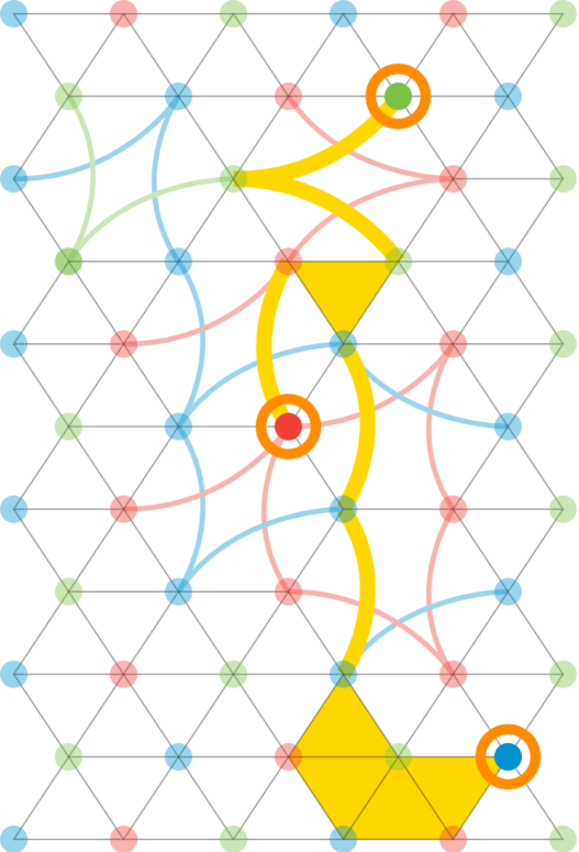
We consider phase-flip noise as the correction of bit-flips is analogous and can be done separately. Let $\widetilde{\mathcal{L}}$ denote a 2D HCT code lattice, produced from a color code lattice $\mathcal{L}$ (without boundary) by morphing some subset of its ball-like regions. We label the three colors of the vertices by $r$, $b$, and $g$. We use the canonical geometric picture from Section III.1, so qubits in $\widetilde{\mathcal{L}}$ are associated with $rgb$-faces, i.e., faces $f\in\widetilde{\mathcal{L}}_{2}\cap\mathcal{L}_{2}$ and $cc$-edges, i.e., edges $e\in\widetilde{\mathcal{L}}_{1}\setminus\mathcal{L}_{1}$. And $X$-type stabilizer generators are associated with vertices $v\in\widetilde{\mathcal{L}}_{0}$. We emphasize that $\widetilde{\mathcal{L}}$ should not be treated as a topological object but rather as a combinatorial object. We also make use of a well-known concept in color code decoding: restricted lattices Bombín and Martin-Delgado 2006; Kubica and Delfosse 2019. Let $\widetilde{\mathcal{L}}^{c_{1}c_{2}}$ be the lattice formed from $\widetilde{\mathcal{L}}$ by deleting all vertices of color $c\neq c_{1}\neq c_{2}$, along with all edges and faces that contain these vertices.

We can now state our decoding problem: given an error syndrome $\sigma\subseteq\widetilde{\mathcal{L}}_{0}$ caused by an unknown phase-flip error $\epsilon\subseteq(\widetilde{\mathcal{L}}_{2}\cap\mathcal{L}_{2})\cup(\widetilde{\mathcal{L}}_{1}\setminus\mathcal{L}_{1})$, output a correction operator $\zeta\subseteq(\widetilde{\mathcal{L}}_{2}\cap\mathcal{L}_{2})\cup(\widetilde{\mathcal{L}}_{1}\setminus\mathcal{L}_{1})$ with the same syndrome as $\epsilon$. Decoding is successful if $\zeta$ and $\epsilon$ differ by a stabilizer. Our decoding algorithm consists of the following three steps.

1. 1.

   Matching: we use MWPM to pair up the vertices of $\sigma$ in the restricted lattices $\widetilde{\mathcal{L}}^{rg}$ and $\widetilde{\mathcal{L}}^{rb}$. That is, we obtain a set of edges $E^{rg}\subseteq\widetilde{\mathcal{L}}_{1}^{rg}$ whose boundary is exactly $\sigma\cap\widetilde{\mathcal{L}}_{0}^{rg}$ (and similarly for $\widetilde{\mathcal{L}}^{rb}$). In a slight abuse of terminology, we call such a set of edges a matching.

2. 2.

   Local Modification: we modify the matchings as follows, focusing on $E^{rg}$ (for $E^{rb}$ exchange $g\leftrightarrow b$ below). For each $rr$-edge $e\in E^{rg}$, we find the color $c$ of its corresponding ball-like region $\mathcal{B}^{v}$ in $\mathcal{L}$. If $c\neq g$, we remove $e$ from the matching. Let $u_{1}$ and $u_{2}$ be the endpoints of $e$. We find two vertices $w_{1},w_{2}\in\widetilde{\mathcal{L}}_{0}$ such that $(u_{1},w_{1},v)$ and $(u_{2},w_{2},v)$ are contained in $\mathcal{L}_{2}$ for some $v\in\mathcal{L}_{0}$. Then we find a path $(e_{1},\ldots,e_{m})$ from $w_{1}$ to $w_{2}$ consisting of $gg$-edges. We add the edges $(u_{1},w_{1})$, $(u_{2},w_{2})$, $e_{1},\ldots,e_{m}$ to the matching.

3. 3.

   Local Lift: first, we add each $cc$-edge in the combined matching $E^{rg}\cup E^{rb}$ to the correction $\zeta$. Then, for each $r$-vertex $v\in e$ such that $e\in E^{rg}\cup E^{rb}$ we apply a local lift. For regions of $\widetilde{\mathcal{L}}$ that are the same as the corresponding regions $\mathcal{L}$, the local lift is the color code lift described in Kubica and Delfosse 2019. In the morphed regions of $\widetilde{\mathcal{L}}$, the local lift must be modified to account for the changes due to morphing; see Appendix G. Let $\zeta_{v}\subseteq(\widetilde{\mathcal{L}}_{2}\cap\mathcal{L}_{2})\cup(\widetilde{\mathcal{L}}_{1}\setminus\mathcal{L}_{1})$ be the output of the local lift at $v$. We update the correction $\zeta=\zeta\bigtriangleup\zeta_{v}$.

Figure 7 illustrates our algorithm via and example, and a C++ implementation of our algorithm (utilizing Blossom V Kolmogorov 2009) is available online git. We can now explain our earlier statement that morphing can simplify the decoding problem. Morphing (applied judiciously) transforms a color code into copies of the toric code, changing the decoding problem from color code decoding to the simpler toric code decoding problem. In particular, the local lift in the toric code regions is trivial, compared with the local lift in the color code regions. Therefore one can argue that the decoding problem is simplified in the regions of the lattice that have been morphed.

Our algorithm has runtime complexity $O(N^{3})$ (see Appendix G), where $N$ is the number of physical qubits in the code, due to the MWPM subroutine. As with the restriction decoder, MWPM can be replaced with any algorithm for 2D toric code decoding. For example, replacing MWPM with union-find Delfosse and Nickerson 2017 would give our algorithm almost linear time complexity. We note that our decoder is an instance of the ‘decoding using emergent symmetries’ paradigm, which underlies many topological code decoders Kubica and Delfosse 2019; Brown and Williamson 2020; Bonilla Ataides et al. 2021. As in the color code, the emergent symmetries in our case are the products of all stabilizers of the same color.

One example application for our decoder is color code-toric code lattice surgery Poulsen Nautrup et al. 2017. There can be advantages to preparing magic states in a color code before transferring them to a toric code Shutty and Chamberland 2022. This transfer is accomplished via lattice surgery, during which the color code and toric code will be temporarily merged to form an HCT code that must be decoded as part of the lattice surgery protocol. For our decoder to be directly applicable to this situation, we would need to modify our algorithm to work for codes with boundaries, but we expect that this modification would proceed in a similar way to the restriction decoder Chamberland et al. 2020b.

We investigate the performance of our decoding algorithm using Monte Carlo simulations. We begin with the family of 2D color codes defined on $L\times L$ triangular tilings where six triangles meet at each vertex. We use periodic boundary conditions, i.e., we identify the coordinates $(x,y)=(x+L,y)=(x,y+L)=(x+L,y+L)$. From this starting point, we explore three ways of constructing HCT codes.

1. 1.

   Method A: We choose $q\in[0,1]$ and construct a random HCT code by morphing each $r$ ball-like region with probability $q$. We consider both choosing the same logical Pauli basis for each region (A1), and choosing the basis randomly (A2).

2. 2.

   Method B: We choose $q\in[0,1]$ and iterate through the $r$ ball-like regions, morphing with probability $q$. Next we iterate through the $g$ ball-like regions and morph with probability $q$, except if an overlapping region has already been morphed. Lastly, we iterate through the $b$ ball-like regions and morph with probability $q$ (again unless an overlapping region has already been morphed). In all cases we choose the logical Pauli basis randomly.

3. 3.

   Method C: We choose $q\in[0,1]$ and put the vertices of the lattice into a random order. For each vertex in the list, with probability $q$ we morph the ball-like region centred at the vertex (choosing the logical Pauli basis randomly), except if an overlapping region has already been morphed.

By definition, the parameter $q$ captures the proportion of morphed $r$ ball-like regions in Methods A1, A2 and B. However in Method C the parameter $q$ does not correspond directly to the proportion of morphed ball-like regions because of the non-overlapping condition. Furthermore, in the $q=1$ limit Methods A1, A2 and B all produce toric codes with certainty, whereas Method C with high probability does not produce a toric code as this would require all the vertices of one color to occur at the start of the random ordering.

We investigate the performance of our decoder as a function of $q$ for each of the above methods. In each case, we use an error model where iid $Z$ errors affect the qubits with probability $p$ and stabilizer measurements are perfect. We use Monte Carlo simulations to estimate the logical error rate $p_{\mathrm{fail}}$ as a function of $p$, $L$, and $q$; see Fig. 8a. For each value of $q>0$, we randomly generate 100 HCT code lattices for each $L$, and for each value of $p$ we carry out 1000 Monte Carlo trials per lattice. For each value of $q$, we estimate the error threshold $p_{\mathrm{th}}(q)$ using finite-size scaling methods Harrington 2004, as illustrated in Fig. 8b.

For Method A1, we reproduce the known color code error threshold of $p_{\mathrm{fail}}(0)\approx 0.085$ Delfosse 2014 and the known toric code threshold of $p_{\mathrm{fail}}(1)\approx 0.103$ Wang et al. 2003. The threshold monotonically increases from $q=0$ to $q=1$; see Fig. 8c. For Method A2 we observe an increased threshold of $p_{\mathrm{fail}}(1)\approx 0.105$; see Fig. 8c This is not surprising, as by picking the logical Pauli basis randomly we are highly unlikely to produce the standard square lattice toric code for $q=1$.

For Method B, we observe similar results to the case where we morphed only $r$ ball-like regions using random logical Pauli bases. And for Method C, we find that the error threshold does not vary with $q$ and is approximately equal to the color code error threshold of $p_{\mathrm{fail}}(0)\approx 0.085$. The data for these cases are shown in Fig. 8c.

References

- Aharonov and Ben-Or (2008) D. Aharonov and M. Ben-Or, Fault-Tolerant Quantum Computation with Constant Error Rate, SIAM Journal on Computing 38, 1207 (2008).
- Knill et al. (1998) E. Knill, R. Laflamme, and W. H. Zurek, Resilient Quantum Computation, Science 279, 342 (1998).
- Kitaev (1997a) A. Y. Kitaev, Quantum computations: Algorithms and error correction, Russian Mathematical Surveys 52, 1191 (1997a).
- Gottesman (2014) D. Gottesman, Fault-tolerant quantum computation with constant overhead, Quantum Information & Computation 14, 1338 (2014), arXiv:1310.2984 .
- Fawzi et al. (2018) O. Fawzi, A. Grospellier, and A. Leverrier, Constant Overhead Quantum Fault-Tolerance with Quantum Expander Codes, in 2018 IEEE 59th Annual Symposium on Foundations of Computer Science (FOCS) (IEEE, Paris, 2018) pp. 743–754.
- Litinski (2019a) D. Litinski, A Game of Surface Codes: Large-Scale Quantum Computing with Lattice Surgery, Quantum 3, 128 (2019a), arXiv:1808.02892 .
- Fowler and Gidney (2019) A. G. Fowler and C. Gidney, Low overhead quantum computation using lattice surgery, arXiv preprint (2019), arXiv:1808.06709 .
- Chamberland et al. (2020a) C. Chamberland, K. Noh, P. Arrangoiz-Arriola, E. T. Campbell, C. T. Hann, J. Iverson, H. Putterman, T. C. Bohdanowicz, S. T. Flammia, A. Keller, G. Refael, J. Preskill, L. Jiang, A. H. Safavi-Naeini, O. Painter, and F. G. S. L. Brandão, Building a fault-tolerant quantum computer using concatenated cat codes, arXiv preprint (2020a), arXiv:2012.04108 .
- Kim et al. (2021) I. H. Kim, E. Lee, Y.-H. Liu, S. Pallister, W. Pol, and S. Roberts, Fault-tolerant resource estimate for quantum chemical simulations: Case study on Li-ion battery electrolyte molecules, arXiv preprint (2021), arXiv:2104.10653 .
- Beverland et al. (2021) M. E. Beverland, A. Kubica, and K. M. Svore, Cost of Universality: A Comparative Study of the Overhead of State Distillation and Code Switching with Color Codes, PRX Quantum 2, 020341 (2021).
- Egan et al. (2021) L. Egan, D. M. Debroy, C. Noel, A. Risinger, D. Zhu, D. Biswas, M. Newman, M. Li, K. R. Brown, M. Cetina, and C. Monroe, Fault-Tolerant Operation of a Quantum Error-Correction Code, arXiv preprint (2021), arXiv:2009.11482 .
- Andersen et al. (2020) C. K. Andersen, A. Remm, S. Lazar, S. Krinner, N. Lacroix, G. J. Norris, M. Gabureac, C. Eichler, and A. Wallraff, Repeated quantum error detection in a surface code, Nature Physics 16, 875 (2020).
- Chen et al. (2021a) Z. Chen, K. J. Satzinger, J. Atalaya, A. N. Korotkov, A. Dunsworth, D. Sank, C. Quintana, M. McEwen, R. Barends, P. V. Klimov, S. Hong, C. Jones, A. Petukhov, D. Kafri, S. Demura, B. Burkett, C. Gidney, A. G. Fowler, A. Paler, H. Putterman, I. Aleiner, F. Arute, K. Arya, R. Babbush, J. C. Bardin, A. Bengtsson, A. Bourassa, M. Broughton, B. B. Buckley, D. A. Buell, N. Bushnell, B. Chiaro, R. Collins, W. Courtney, A. R. Derk, D. Eppens, C. Erickson, E. Farhi, B. Foxen, M. Giustina, A. Greene, J. A. Gross, M. P. Harrigan, S. D. Harrington, J. Hilton, A. Ho, T. Huang, W. J. Huggins, L. B. Ioffe, S. V. Isakov, E. Jeffrey, Z. Jiang, K. Kechedzhi, S. Kim, A. Kitaev, F. Kostritsa, D. Landhuis, P. Laptev, E. Lucero, O. Martin, J. R. McClean, T. McCourt, X. Mi, K. C. Miao, M. Mohseni, S. Montazeri, W. Mruczkiewicz, J. Mutus, O. Naaman, M. Neeley, C. Neill, M. Newman, M. Y. Niu, T. E. O’Brien, A. Opremcak, E. Ostby, B. Pató, N. Redd, P. Roushan, N. C. Rubin, V. Shvarts, D. Strain, M. Szalay, M. D. Trevithick, B. Villalonga, T. White, Z. J. Yao, P. Yeh, J. Yoo, A. Zalcman, H. Neven, S. Boixo, V. Smelyanskiy, Y. Chen, A. Megrant, J. Kelly, and Google Quantum AI, Exponential suppression of bit or phase errors with cyclic error correction, Nature 595, 383 (2021a).
- Chen et al. (2021b) E. H. Chen, T. J. Yoder, Y. Kim, N. Sundaresan, S. Srinivasan, M. Li, A. D. Córcoles, A. W. Cross, and M. Takita, Calibrated decoders for experimental quantum error correction, arXiv preprint (2021b), arXiv:2110.04285 .
- Erhard et al. (2021) A. Erhard, H. Poulsen Nautrup, M. Meth, L. Postler, R. Stricker, M. Stadler, V. Negnevitsky, M. Ringbauer, P. Schindler, H. J. Briegel, R. Blatt, N. Friis, and T. Monz, Entangling logical qubits with lattice surgery, Nature 589, 220 (2021).
- Bravyi and Kitaev (2005) S. Bravyi and A. Kitaev, Universal quantum computation with ideal Clifford gates and noisy ancillas, Physical Review A 71, 022316 (2005).
- Meier et al. (2013) A. M. Meier, B. Eastin, and E. Knill, Magic-state distillation with the four-qubit code, Quantum Information & Computation 13, 195–209 (2013), arXiv:1204.4221 .
- Bombín and Martin-Delgado (2006) H. Bombín and M. A. Martin-Delgado, Topological Quantum Distillation, Physical Review Letters 97, 180501 (2006).
- Bombín and Martin-Delgado (2007a) H. Bombín and M. A. Martin-Delgado, Topological Computation without Braiding, Physical Review Letters 98, 160502 (2007a).
- Kubica (2018) A. M. Kubica, The ABCs of the Color Code: A Study of Topological Quantum Codes as Toy Models for Fault-Tolerant Quantum Computation and Quantum Phases of Matter, Ph.D. thesis, Caltech (2018).
- Kubica et al. (2015) A. Kubica, B. Yoshida, and F. Pastawski, Unfolding the color code, New Journal of Physics 17, 083026 (2015).
- Vasmer and Browne (2019) M. Vasmer and D. E. Browne, Three-dimensional surface codes: Transversal gates and fault-tolerant architectures, Physical Review A 100, 012312 (2019).
- Jochym-O’Connor and Yoder (2021) T. Jochym-O’Connor and T. J. Yoder, A four-dimensional toric code with non-Clifford transversal gates, Physical Review Research 3, 013118 (2021), arXiv:2010.02238 .
- Dennis et al. (2002) E. Dennis, A. Kitaev, A. Landahl, and J. Preskill, Topological quantum memory, Journal of Mathematical Physics 43, 4452 (2002).
- Fowler (2015) A. G. Fowler, Minimum weight perfect matching of fault-tolerant topological quantum error correction in average O(1) parallel time, Quantum Information & Computation 15, 145 (2015), arXiv:1307.1740 .
- Kubica and Delfosse (2019) A. Kubica and N. Delfosse, Efficient color code decoders in $d\geq 2$ dimensions from toric code decoders, arXiv preprint (2019), arXiv:1905.07393 .
- Gottesman (1997) D. Gottesman, Stabilizer Codes and Quantum Error Correction, arXiv preprint (1997), arXiv:quant-ph/9705052 .
- (28) We observe that morphing is similar to the disentangling step of entanglement renormalization Vidal 2007.
- Steane (1996) A. M. Steane, Multiple-particle interference and quantum error correction, Proceedings of the Royal Society of London. Series A: Mathematical, Physical and Engineering Sciences 452, 2551 (1996).
- Knill (2005) E. Knill, Quantum computing with realistically noisy devices, Nature 434, 39 (2005).
- Knill (2004) E. Knill, Fault-Tolerant Postselected Quantum Computation: Schemes, arXiv preprint (2004), arXiv:quant-ph/0402171 .
- Bravyi and Haah (2012) S. Bravyi and J. Haah, Magic-state distillation with low overhead, Physical Review A 86, 052329 (2012).
- Campbell and Howard (2017a) E. T. Campbell and M. Howard, Unifying Gate Synthesis and Magic State Distillation, Physical Review Letters 118, 060501 (2017a).
- Hastings and Haah (2018) M. B. Hastings and J. Haah, Distillation with Sublogarithmic Overhead, Physical Review Letters 120, 050504 (2018).
- Haah et al. (2017) J. Haah, M. B. Hastings, D. Poulin, and D. Wecker, Magic State Distillation at Intermediate Size, Quantum Information and Computation 18, 10.26421/QIC18.1-2 (2017), arXiv:1709.02789 .
- Haah and Hastings (2018) J. Haah and M. B. Hastings, Codes and Protocols for Distilling $T$, controlled-$S$, and Toffoli Gates, Quantum 2, 71 (2018), arXiv:1709.02832 .
- Steane (1999) A. Steane, Quantum Reed-Muller codes, IEEE Transactions on Information Theory 45, 1701 (1999).
- Anderson et al. (2014) J. T. Anderson, G. Duclos-Cianci, and D. Poulin, Fault-Tolerant Conversion between the Steane and Reed-Muller Quantum Codes, Physical Review Letters 113, 080501 (2014).
- MacWilliams and Sloane (1977) F. J. MacWilliams and N. J. A. Sloane, The Theory of Error Correcting Codes, North-Holland Mathematical Library ; v. 16 (North-Holland Pub. Co., Amsterdam, 1977).
- Campbell (2016) E. T. Campbell, The smallest interesting colour code, https://earltcampbell.com/2016/09/26/the-smallest-interesting-colour-code/ (2016), accessed: 2021-07-20.
- Paetznick and Reichardt (2013) A. Paetznick and B. W. Reichardt, Universal Fault-Tolerant Quantum Computation with Only Transversal Gates and Error Correction, Physical Review Letters 111, 090505 (2013).
- Jones (2013) C. Jones, Low-overhead constructions for the fault-tolerant Toffoli gate, Physical Review A 87, 022328 (2013).
- Litinski (2019b) D. Litinski, Magic State Distillation: Not as Costly as You Think, Quantum 3, 205 (2019b), arXiv:1905.06903 .
- Gidney and Fowler (2019) C. Gidney and A. G. Fowler, Efficient magic state factories with a catalyzed —CCZ to 2—T transformation, Quantum 3, 135 (2019), arXiv:1812.01238 .
- Campbell and Howard (2017b) E. T. Campbell and M. Howard, Unified framework for magic state distillation and multiqubit gate synthesis with reduced resource cost, Physical Review A 95, 022316 (2017b).
- Bombín (2015) H. Bombín, Gauge color codes: Optimal transversal gates and gauge fixing in topological stabilizer codes, New Journal of Physics 17, 083002 (2015).
- Kubica and Beverland (2015) A. Kubica and M. E. Beverland, Universal transversal gates with color codes - a simplified approach, Physical Review A 91, 032330 (2015), arXiv:1410.0069 .
- Watson et al. (2015) F. H. E. Watson, E. T. Campbell, H. Anwar, and D. E. Browne, Qudit color codes and gauge color codes in all spatial dimensions, Physical Review A 92, 022312 (2015).
- Bombín (2018) H. Bombín, Transversal gates and error propagation in 3D topological codes, arXiv preprint (2018), arXiv:1810.09575 .
- Criger and Terhal (2016) B. Criger and B. Terhal, Noise Thresholds for the [[4, 2, 2]]-concatenated Toric Code, Quantum Information and Computation 16, 10.26421/QIC16.15-16 (2016), arXiv:1604.04062 .
- Bombín et al. (2012) H. Bombín, G. Duclos-Cianci, and D. Poulin, Universal topological phase of two-dimensional stabilizer codes, New Journal of Physics 14, 073048 (2012).
- Delfosse (2014) N. Delfosse, Decoding color codes by projection onto surface codes, Physical Review A 89, 012317 (2014), arXiv:1308.6207 .
- Kolmogorov (2009) V. Kolmogorov, Blossom V: A new implementation of a minimum cost perfect matching algorithm, Mathematical Programming Computation 1, 43 (2009).
- (54) https://github.com/MikeVasmer/hybrid-decoder.
- Delfosse and Nickerson (2017) N. Delfosse and N. H. Nickerson, Almost-linear time decoding algorithm for topological codes, arXiv preprint (2017), arXiv:1709.06218 .
- Brown and Williamson (2020) B. J. Brown and D. J. Williamson, Parallelized quantum error correction with fracton topological codes, Physical Review Research 2, 013303 (2020), arXiv:1901.08061 .
- Bonilla Ataides et al. (2021) J. P. Bonilla Ataides, D. K. Tuckett, S. D. Bartlett, S. T. Flammia, and B. J. Brown, The XZZX surface code, Nature Communications 12, 2172 (2021), arXiv:2009.07851 .
- Poulsen Nautrup et al. (2017) H. Poulsen Nautrup, N. Friis, and H. J. Briegel, Fault-tolerant interface between quantum memories and quantum processors, Nature Communications 8, 1321 (2017).
- Shutty and Chamberland (2022) N. Shutty and C. Chamberland, Finding fault-tolerant Clifford circuits using satisfiability modulo theories solvers and decoding merged color-surface codes, arXiv preprint (2022), arXiv:2201.12450 .
- Chamberland et al. (2020b) C. Chamberland, A. Kubica, T. J. Yoder, and G. Zhu, Triangular color codes on trivalent graphs with flag qubits, New Journal of Physics 22, 023019 (2020b), arXiv:1911.00355 .
- Harrington (2004) J. Harrington, Analysis of Quantum Error-Correcting Codes Symplectic Lattice Codes and Toric Codes, Ph.D. thesis, Caltech (2004).
- Wang et al. (2003) C. Wang, J. Harrington, and J. Preskill, Confinement-Higgs transition in a disordered gauge theory and the accuracy threshold for quantum memory, Annals of Physics 303, 31 (2003), arXiv:quant-ph/0207088 .
- Iverson (2020) J. K. Iverson, Aspects of Fault-Tolerant Quantum Computation, Ph.D. thesis, Caltech (2020).
- Iverson and Kubica (2022) J. Iverson and A. Kubica, (2022), in preparation.
- Raussendorf and Harrington (2007) R. Raussendorf and J. Harrington, Fault-Tolerant Quantum Computation with High Threshold in Two Dimensions, Physical Review Letters 98, 190504 (2007).
- Wang et al. (2010) D. S. Wang, A. G. Fowler, A. M. Stephens, and L. C. L. Hollenberg, Threshold error rates for the toric and planar codes, Quantum Information & Computation 10, 456 (2010), arXiv:0905.0531 .
- Bravyi et al. (2014) S. Bravyi, M. Suchara, and A. Vargo, Efficient algorithms for maximum likelihood decoding in the surface code, Physical Review A 90, 032326 (2014).
- Chubb (2021) C. T. Chubb, General tensor network decoding of 2D Pauli codes, arXiv preprint (2021), arXiv:2101.04125 .
- Katzgraber et al. (2009) H. G. Katzgraber, H. Bombín, and M. A. Martin-Delgado, Error Threshold for Color Codes and Random Three-Body Ising Models, Physical Review Letters 103, 090501 (2009).
- Honecker et al. (2001) A. Honecker, M. Picco, and P. Pujol, Universality Class of the Nishimori Point in the 2D $\pm J$ Random-Bond Ising Model, Physical Review Letters 87, 047201 (2001).
- Merz and Chalker (2002) F. Merz and J. T. Chalker, Two-dimensional random-bond Ising model, free fermions, and the network model, Physical Review B 65, 054425 (2002).
- Ohzeki (2009) M. Ohzeki, Locations of multicritical points for spin glasses on regular lattices, Physical Review E 79, 021129 (2009), arXiv:0811.0464 .
- Poulin (2005) D. Poulin, Stabilizer Formalism for Operator Quantum Error Correction, Physical Review Letters 95, 230504 (2005).
- Kubica and Vasmer (2021) A. Kubica and M. Vasmer, Single-shot quantum error correction with the three-dimensional subsystem toric code, arXiv preprint (2021), arXiv:2106.02621 .
- Vuillot and Breuckmann (2019) C. Vuillot and N. P. Breuckmann, Quantum Pin Codes, arXiv preprint (2019), arXiv:1906.11394 .
- Bombín and Martin-Delgado (2007b) H. Bombín and M. A. Martin-Delgado, Exact topological quantum order in D = 3 and beyond: Branyons and brane-net condensates, Physical Review B 75, 075103 (2007b).
- Kitaev (1997b) A. Y. Kitaev, Quantum Error Correction with Imperfect Gates, in Quantum Communication, Computing, and Measurement, edited by O. Hirota, A. S. Holevo, and C. M. Caves (Springer US, Boston, MA, 1997) pp. 181–188.
- Kitaev (2003) A. Y. Kitaev, Fault-tolerant quantum computation by anyons, Annals of Physics 303, 2 (2003), arXiv:quant-ph/9707021 .
- Calderbank and Shor (1996) A. R. Calderbank and P. W. Shor, Good quantum error-correcting codes exist, Physical Review A 54, 1098 (1996).
- Krishna and Tillich (2019) A. Krishna and J.-P. Tillich, Towards Low Overhead Magic State Distillation, Physical Review Letters 123, 070507 (2019).
- Coxeter (1973) H. S. M. Coxeter, Regular Polytopes (Dover, New York, 1973).
- Vasmer (2019) M. Vasmer, Fault-Tolerant Quantum Computing with Three-Dimensional Surface Codes, Ph.D. thesis, University College London (2019).
- Breuckmann and Terhal (2016) N. P. Breuckmann and B. M. Terhal, Constructions and Noise Threshold of Hyperbolic Surface Codes, IEEE Transactions on Information Theory 62, 3731 (2016), arXiv:1506.04029 .
- Breuckmann et al. (2017) N. P. Breuckmann, C. Vuillot, E. Campbell, A. Krishna, and B. M. Terhal, Hyperbolic and semi-hyperbolic surface codes for quantum storage, Quantum Science and Technology 2, 035007 (2017).
- Breuckmann (2018) N. P. Breuckmann, PhD thesis: Homological Quantum Codes Beyond the Toric Code, arXiv preprint (2018), arXiv:1802.01520 .
- Humphreys (1990) J. E. Humphreys, Reflection Groups and Coxeter Groups, 1st ed. (Cambridge University Press, 1990).
- Davis (2008) M. Davis, The Geometry and Topology of Coxeter Groups, London Mathematical Society Monographs Series (Princeton University Press, Princeton, 2008).
- Brown et al. (2016) B. J. Brown, N. H. Nickerson, and D. E. Browne, Fault-tolerant error correction with the gauge color code, Nature Communications 7, 12302 (2016).
- Kesselring et al. (2018) M. S. Kesselring, F. Pastawski, J. Eisert, and B. J. Brown, The boundaries and twist defects of the color code and their applications to topological quantum computation, Quantum 2, 101 (2018), arXiv:1806.02820 .
- Bombín (2010) H. Bombín, Topological Order with a Twist: Ising Anyons from an Abelian Model, Physical Review Letters 105, 030403 (2010).
- Vidal (2007) G. Vidal, Entanglement renormalization, Phys. Rev. Lett. 99, 220405 (2007).