MegBA: A GPU-Based Distributed Library for Large-Scale Bundle Adjustment

We focus on partitioning the Hessian matrix produced in BA. For example, in a BA dataset with 80M edges, a Hessian matrix $\boldsymbol{H}$ consume over 50G memory, leading to over 99.9% storage to be allocated to $\boldsymbol{E}$ and $\boldsymbol{E}^{T}$. We want to have a generic method that partitions the Hessian matrix in a BA problem. This method needs to assign each parallel device with a part of the matrix $\boldsymbol{E}$ and $\boldsymbol{E}^{T}$, preferably in equal sizes. The partitioning needs to guarantee that the global solution merged from local solutions is equivalent to the one computed using a single node. This equivalence property is the key to ensuring a high-precision solution found by MegBA.

At the high level, MegBA achieves distributed BA using two major components: (i) a method that can divide a BA problem into sub-problems, and (ii) an algorithm that can coordinate distributed PCG algorithms to solve sub-problems in parallel. Our partitioning method is based on a key observation in BA problems: the non-zero blocks in $\boldsymbol{E}$ and $\boldsymbol{E}^{T}$ are corresponding with edges, i.e., the $i$-th row $j$-th column non-zero block in $\boldsymbol{E}$ is computed by $e_{i,j}$, we can partition edges based on the number of available GPUs, and each GPU only store part of these non-zero blocks (We provide an example to illustrate the partitioning process in the supplementary materials).

Assume there are $K$ GPUs, given a BA problem, we tile edges to a vector $\boldsymbol{e}=\begin{array}[]{ccc}[\dots&e_{i,j}&\dots]^{T}\end{array}$, then we partition it to several blocks $\boldsymbol{e}=\begin{array}[]{cccc}[\boldsymbol{e}_{1}^{T}&\boldsymbol{e}_{2}^{T}&\dots&\boldsymbol{e}_{K}^{T}]^{T}\end{array}$. The Jacobian $\boldsymbol{J}$ could be partitioned into several blocks:

Assuming identity information matrix is given here, Hessian $\boldsymbol{H}$ can be partitioned:

To perform Schur elimination, we represented $\boldsymbol{H}_{k}$ as sub-blocks:

Matrix blocks in Equation 2 have the following equivalent forms in the edge-based partition setting: $\boldsymbol{B}=\sum_{k=1}^{K}\boldsymbol{B}_{k}$, $\boldsymbol{E}=\sum_{k=1}^{K}\boldsymbol{E}_{k}$, $\boldsymbol{E}^{T}=\sum_{k=1}^{K}\boldsymbol{E}_{k}^{T}$, and $\boldsymbol{C}=\sum_{k=1}^{K}\boldsymbol{C}_{k}$. The number of non-zero parameter blocks in $\boldsymbol{E}$ or $\boldsymbol{E}^{T}$ equals the number of edges. Notably, the sub-matrices $\boldsymbol{B}_{k}$ and $\boldsymbol{C}_{k}$ have the same number of non-zero elements as $\boldsymbol{B}$ and $\boldsymbol{C}$, respectively. Since we store matrices in the Compressed Sparse Row (CSR) format, each GPU only stores $\frac{1}{K}$ non-zero blocks in $\boldsymbol{E}$ and $\boldsymbol{E}^{T}$. The blocking strategy greatly alleviates the problem that $\boldsymbol{E}$ and $\boldsymbol{E}^{T}$ are too large to be stored on a single device.

By applying the above partition method for Equation 2, an equivalent distributed version can be formulated as follow:

By far we have partitioned a BA problem and assigned sub-problems to all GPUs. In the following, we will discuss how does MegBA coordinates the solving of sub-problems in a distributed manner.

Algorithm 1 introduces the overall distributed BA algorithm in MegBA. The distributed BA algorithm takes as initial state and partitioned edges as described in Section 8. We use JecVector to compute the Jacobian and residual (Line 2). JetVector is a novel data structure to represent BA data in a SIMD format, it can make full use of the hardware characteristics of GPU (e.g. coalesced memory loading) to do auto-differentiation over millions of edges in parallel. We give a more detailed illustration in Section 5.1. Then we build a linear system (Line 3). We perform allreduce [25] on diagonal-blocks and constant vector (Line 4) before solving the linear system because the size of diagonal-blocks and constant vector is small and they would be used several times in the following procedures.

We then compute constant vector in Equation 3 (Line 5-7) and solve the linear system by using a Distributed PCG (DPCG) algorithm (Line 8). Notably, we do necessary allreduce in the DPCG algorithm to guarantee DPCG output the same result as non-distributed PCG solver does in solving Equation 3, further implementation details will be shown in Section 4.3. After solving the linear system in Equation 3, we compute the increment of $\boldsymbol{x}_{p}$ following Equation 4 (Line 9-11). Once we have computed the increment $\Delta\boldsymbol{x}_{c}$ and $\Delta\boldsymbol{x}_{p}$, we update the state $\boldsymbol{x}_{c}$ and $\boldsymbol{x}_{p}$ (Line 12). If it doesn’t satisfy the convergence criteria we will start another loop; otherwise, we will return the optimised state $\boldsymbol{x}$.

We then discuss how to distribute the PCG algorithm in BA, shown in Algorithm 1. This algorithm first constructs a linear system defined in Equation 2. It then solves Equation 3 and computes increment following Equation 4. It finally uses the increments update state $\boldsymbol{x}$, and tested if a convergence criterion has been met. To guarantee that the distributed BA algorithm achieves the convergence performance, we make Algorithm 1, named DPCG, return the same result as the non-distributed linear solver.

In the following, we describe the execution of DPCG. DPCG takes BA initial state $\boldsymbol{x}^{0}$, matrix block $\boldsymbol{B}$, $\boldsymbol{E}_{k}$, $\boldsymbol{E}_{k}^{T}$, $\boldsymbol{C}$ of $\boldsymbol{H}_{k}$, constant vector $\boldsymbol{b}$ as input and output solution $\boldsymbol{x}$ for linear system [$\boldsymbol{B}-\boldsymbol{E}\boldsymbol{C}^{-1}\boldsymbol{E}^{T}]\boldsymbol{x}=\boldsymbol{b}$, where $\boldsymbol{E}=\sum_{k=1}^{K}\boldsymbol{E}_{k}$ and $\boldsymbol{E}^{T}=\sum_{k=1}^{K}\boldsymbol{E}_{k}$. The procedures of DPCG using Schur elimination is similar to single-node PCG. Notably, the coefficient matrix of the linear system to be solved is Schur complement. The matrix-vector multiplication operations (Line 1, 12 in Algorithm 2) is thus the multiplication between Schur complement and vector. The difference between distributed compared with non-distributed setting is that DPCG only assign $\boldsymbol{E}_{k}$ and $\boldsymbol{E}_{k}^{T}$ rather than the complete matrices $\boldsymbol{E}$ and $\boldsymbol{E}^{T}$ to GPU $k$, so we need to guarantee operations that use $\boldsymbol{E}_{k}$ and $\boldsymbol{E}_{k}^{T}$ have the same output compared with using $\boldsymbol{E}$ and $\boldsymbol{E}^{T}$, these operations happen when doing Schur elimination (Line 1, 12).

Our key idea of computing Schur elimination in a distributed manner is that: the summation of matrix-vector multiplication is the same as the the result matrix summation multiplies vector, i.e., $\sum_{k=1}^{K}(\boldsymbol{E}_{k}\boldsymbol{v})=\sum_{k=1}^{K}(\boldsymbol{E}_{k})\boldsymbol{v}$. We compute an intermediate vector (Line 1) and reduce it (Line 2), then we compute intermediate vectors sequentially (Line 3, 4). We perform all-reduce operation over the intermediate vector (Line 5) and compute another intermediate vector (Line 6. After those procedures, we do subtraction to the last two intermediate vectors and output the final result. The result would be the same as computing the complete Schur complement $[\boldsymbol{B}-\boldsymbol{E}\boldsymbol{C}^{-1}\boldsymbol{E}]$ then multiplying it with vector $\boldsymbol{x}$.

In the end, we present the complexity analysis of MegBA. Assume that MegBA is given $m$ cameras, $n$ points, and $k$ observations and we often have $k\gg m,n$, the time complexity for building the linear system is $\mathcal{O}(m+n+k)$ and the time complexity for each iteration of the conjugate gradient is $\mathcal{O}(m+n+k)$. Assume we distribute the problem to $K$ GPUs, on each GPU, the time complexity for building the linear system is $\mathcal{O}(m+n+k/K)$ and the time complexity for each iteration of the conjugate gradient is $\mathcal{O}(m+n+k/K)$. The ring all-reduce communication time complexity of each conjugate gradient iteration is $\mathcal{O}(m+n)$. In summary, the total complexity of MegBA is $\mathcal{O}(m+n+k/K)$.

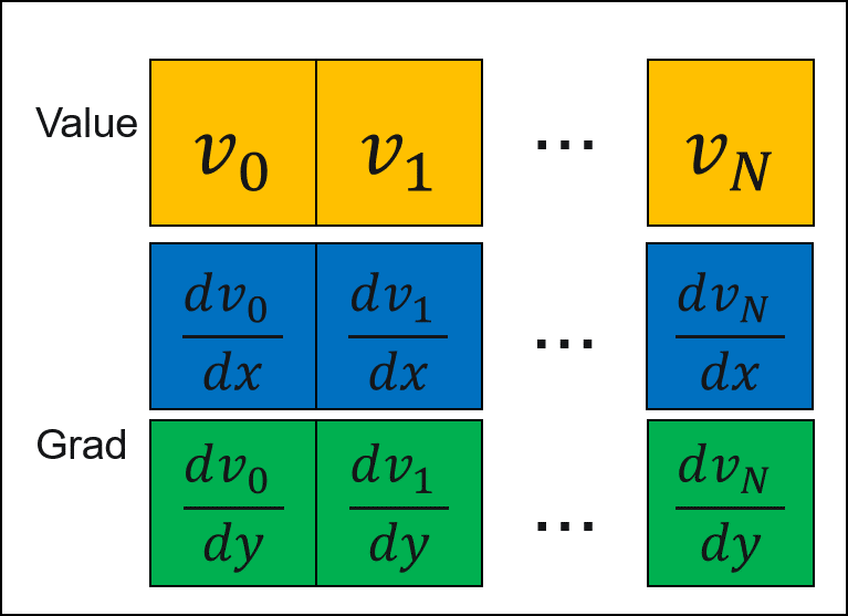
JetVector is a novel data structure to perform auto-differentiation over millions of edges. Compared to conventional BA data structure: Jet implemented in Ceres, JetVector represents a list of Jets (i.e., Array-of-Structure) as a single data object where Jet’s data fields: data and grad across all items are represented as single arrays (i.e., Array-within-Structure). When we perform mathematical operations on JetVector, we will start as many GPU threads as the elements in it, every GPU thread process one element. Because data and grad are stored in the structure of Array-within-Structure, the memory transactions are coalesced and make it easy to reach a high memory throughput. The detailed structure layout of JecVector could be found in supplementary materials.

Besides JetVector, other parts of MegBA are also implemented as SIMD-friendly data structures. The construction of linear system (Line 3 in Algorithm 1) uses L1 cache on GPU to store Jacobian blocks in a SIMD manner. The DPCG algorithm includes a lot of matrix/vector operations which also be benefited from the SIMD structure. A full list of SIMD operations implemented in MegBA can be found in supplementary materials.

BA computation involves massive objects to be allocated in GPU memory. To avoid expensive memory allocation [19], we leverage a key observation in BA computation: The automatic differentiation works on GPU buffers that are in the same size across BA iterations. By monitoring the sizes of GPU buffers used in the forward pass of differentiating the BA errors, we can predict the sizes of all memory buffers involved in future BA iterations. Based on this observation, we can pre-allocate these memory buffers in a memory pool, thus avoiding calling the CUDA driver to allocate memory during runtime.

The APIs of MegBA comprises of two major components:

We first evaluate the overall performance of MegBA, Ceres, g2o, RootBA, and DeepLM. MegBA uses from 1 to 8 GPUs, and CPU-based algorithms use 16 threads. We measure the Mean Squared Error (MSE) in pixels over time.

Figure 2 shows the evaluation results. In the Venice-1778 dataset (Figure 2(a)), MegBA achieves the best performance with 8 GPUs, while DeepLM can only use a single GPU. MegBA completes with 3.34 seconds while Ceres, RootBA, g2o uses 319.0, 73.94, and 890.6 seconds, respectively. It shows the substantial speed-up (95.5$\times$, 22.1$\times$, and 266.6$\times$), which indicates the benefits of fully exploiting GPUs to accelerate BA computation. For GPU-based BA libraries, MegBA can complete with 11.96 seconds while DeepLM spent 24.44 seconds, showing the effectiveness of implementing full vectorisation for BA on a single GPU. With more GPUs, MegBA out-performs DeepLM by 7.316$\times$, which reflects the necessity of adopting multiple GPUs.

Thanks to the vectorisation and distributed BA designs, MegBA becomes the state-of-the-art in the large BA dataset (i.e., Final-13682). As shown in Figure 2(b), MegBA completes in 22.10 seconds, while DeepLM uses 149.6 seconds (6.769$\times$ speed-up), Ceres uses 916 seconds (41.45$\times$ speed-up), g2o uses 13161 seconds (595.5$\times$ speed-up), and RootBA uses 1427 seconds (64.57$\times$ speed-up). In other datasets (Figure 2(c)-(e)), we observe similar speed-up achieved by MegBA, indicating the general effectiveness of our proposed approaches. We omit the discussion of these datasets, and their results are reported in Table 2.

Table 3 further provides the detailed experimental results to show the scalability of MegBA, Ceres and DeepLM. In the Venice-1778 dataset, MegBA can consistently improve its performance by adding GPUs (from 11.96 seconds to 3.34 seconds if we increase the number of GPUs from 1 to 8). In addition, the large dataset (Final-13682) can better show the scalability of MegBA. By increasing the number of GPUs from 4 to 8, the time can be reduced to 22.10 seconds.

The accuracy of solving a BA problem is sensitive to the choice of floating point precision (i.e., 32-bit vs. 64-bit floating points). We further evaluate MegBA in all datasets with 32-bit and 64-bit floating points, and we report the results of Venice-1778 and Final-13682 in Table 4. Other datasets show consistent results and we omit them here. In the dataset of Final-13682, with 4 GPUs, MegBA (FP32) can complete in 4.804 seconds and MegBA (FP64) can complete in 28.70 seconds, while both of them are reaching the same MSE. This shows the exactness of the distributed BA algorithm in MegBA. Even with lower precision, MegBA can reach the same MSE as double-precision; but offering 5.97$\times$ speed up, making MegBA (FP32) be the state-of-the-art in Final-13682.

References

- [1] Agarwal, S., Mierle, K., Others: Ceres solver. http://ceres-solver.org
- [2] Agarwal, S., Snavely, N., Seitz, S.M., Szeliski, R.: Bundle adjustment in the large. In: European conference on computer vision (2010)
- [3] Chen, X., Ma, H., Wan, J., Li, B., Xia, T.: Multi-view 3d object detection network for autonomous driving. In: IEEE conference on Computer Vision and Pattern Recognition (2017)
- [4] Chen, Y., Davis, T.A., Hager, W.W., Rajamanickam, S.: Algorithm 887: Cholmod, supernodal sparse cholesky factorization and update/downdate. ACM Transactions on Mathematical Software (TOMS) (2008)
- [5] Cieslewski, T., Choudhary, S., Scaramuzza, D.: Data-efficient decentralized visual slam. In: IEEE international conference on robotics and automation (2018)
- [6] Demmel, N., Gao, M., Laude, E., Wu, T., Cremers, D.: Distributed photometric bundle adjustment. In: IEEE International Conference on 3D Vision (2020)
- [7] Demmel, N., Sommer, C., Cremers, D., Usenko, V.: Square root bundle adjustment for large-scale reconstruction. In: IEEE Conference on Computer Vision and Pattern Recognition (2021)
- [8] Demmel, N., Sommer, C., Cremers, D., Usenko, V.: Square root bundle adjustment for large-scale reconstruction. In: IEEE/CVF Conference on Computer Vision and Pattern Recognition (2021)
- [9] Eisenstat, S.C.: Efficient implementation of a class of preconditioned conjugate gradient methods. SIAM Journal on Scientific and Statistical Computing (1981)
- [10] Eriksson, A., Bastian, J., Chin, T.J., Isaksson, M.: A consensus-based framework for distributed bundle adjustment. In: IEEE Conference on Computer Vision and Pattern Recognition (2016)
- [11] Fratarcangeli, M., Bradley, D., Gruber, A., Zoss, G., Beeler, T.: Fast nonlinear least squares optimization of large-scale semi-sparse problems. In: Computer Graphics Forum (2020)
- [12] Grisetti, G., Kümmerle, R., Strasdat, H., Konolige, K.: g2o: A general framework for (hyper) graph optimization. In: IEEE International Conference on Robotics and Automation (2011)
- [13] Guennebaud, G., Jacob, B., et al.: Eigen v3. http://eigen.tuxfamily.org (2010)
- [14] Guo, Y., Liu, J., Li, G., Mai, L., Dong, H.: Fast and flexible human pose estimation with hyperpose. In: Proceedings of the 29th ACM International Conference on Multimedia (2021)
- [15] Hackel, T., Savinov, N., Ladicky, L., Wegner, J.D., Schindler, K., Pollefeys, M.: Semantic3d. net: A new large-scale point cloud classification benchmark. arXiv preprint arXiv:1704.03847 (2017)
- [16] Huang, J., Huang, S., Sun, M.: Deeplm: Large-scale nonlinear least squares on deep learning frameworks using stochastic domain decomposition. In: IEEE/CVF Conference on Computer Vision and Pattern Recognition (2021)
- [17] Kaess, M., Johannsson, H., Roberts, R., Ila, V., Leonard, J.J., Dellaert, F.: isam2: Incremental smoothing and mapping using the bayes tree. The International Journal of Robotics Research (2012)
- [18] Kaess, M., Ranganathan, A., Dellaert, F.: isam: Incremental smoothing and mapping. IEEE Transactions on Robotics (2008)
- [19] Koliousis, A., Watcharapichat, P., Weidlich, M., Mai, L., Costa, P., Pietzuch, P.: Crossbow: Scaling deep learning with small batch sizes on multi-gpu servers. Proceedings of the VLDB Endowment
- [20] Konolige, K., Agrawal, M.: Frameslam: From bundle adjustment to real-time visual mapping. IEEE Transactions on Robotics (2008)
- [21] Levinson, J., Askeland, J., Becker, J., Dolson, J., Held, D., Kammel, S., Kolter, J.Z., Langer, D., Pink, O., Pratt, V., et al.: Towards fully autonomous driving: Systems and algorithms. In: IEEE intelligent vehicles symposium (2011)
- [22] Li, P., Chen, X., Shen, S.: Stereo r-cnn based 3d object detection for autonomous driving. In: IEEE/CVF Conference on Computer Vision and Pattern Recognition (2019)
- [23] Liu, H., Chen, M., Zhang, G., Bao, H., Bao, Y.: Ice-ba: Incremental, consistent and efficient bundle adjustment for visual-inertial slam. In: IEEE Conference on Computer Vision and Pattern Recognition (2018)
- [24] Ma, X., Wang, Z., Li, H., Zhang, P., Ouyang, W., Fan, X.: Accurate monocular 3d object detection via color-embedded 3d reconstruction for autonomous driving. In: IEEE/CVF International Conference on Computer Vision (2019)
- [25] Mai, L., Li, G., Wagenländer, M., Fertakis, K., Brabete, A.O., Pietzuch, P.: Kungfu: Making training in distributed machine learning adaptive. In: 14th USENIX Symposium on Operating Systems Design and Implementation (OSDI 20) (2020)
- [26] Marquardt, D.W.: An algorithm for least-squares estimation of nonlinear parameters. Journal of the society for Industrial and Applied Mathematics (1963)
- [27] Mayer, H.: Rpba – robust parallel bundle adjustment based on covariance information (2019)
- [28] Ortiz, J., Pupilli, M., Leutenegger, S., Davison, A.J.: Bundle adjustment on a graph processor. In: IEEE/CVF Conference on Computer Vision and Pattern Recognition (2020)
- [29] Park, Y., Lepetit, V., Woo, W.: Multiple 3d object tracking for augmented reality. In: IEEE/ACM International Symposium on Mixed and Augmented Reality (2008)
- [30] Powell, M.J.: A hybrid method for nonlinear equations. Numerical methods for nonlinear algebraic equations (1970)
- [31] Schönberger, J.L., Frahm, J.M.: Structure-from-motion revisited. In: Conference on Computer Vision and Pattern Recognition (2016)
- [32] Schönberger, J.L., Zheng, E., Pollefeys, M., Frahm, J.M.: Pixelwise view selection for unstructured multi-view stereo. In: European Conference on Computer Vision (2016)
- [33] Tang, C., Tan, P.: Ba-net: Dense bundle adjustment network. arXiv preprint arXiv:1806.04807 (2018)
- [34] Triggs, B., McLauchlan, P.F., Hartley, R.I., Fitzgibbon, A.W.: Bundle adjustment—a modern synthesis. In: International workshop on vision algorithms (1999)
- [35] Vo, M., Narasimhan, S.G., Sheikh, Y.: Spatiotemporal bundle adjustment for dynamic 3d reconstruction. In: IEEE Conference on Computer Vision and Pattern Recognition (2016)
- [36] Wang, H.R., Lei, J., Li, A., Wu, Y.H.: A geometry-based point cloud reduction method for mobile augmented reality system. Journal of Computer Science and Technology (2018)
- [37] Wedderburn, R.W.: Quasi-likelihood functions, generalized linear models, and the gauss—newton method. Biometrika (1974)
- [38] Wilson, K., Snavely, N.: Robust global translations with 1dsfm. In: Proceedings of the European Conference on Computer Vision (2014)
- [39] Wu, C., Agarwal, S., Curless, B., Seitz, S.M.: Multicore bundle adjustment. In: IEEE Conference on Computer Vision and Pattern Recognition (2011)
- [40] Zhang, R., Zhu, S., Fang, T., Quan, L.: Distributed very large scale bundle adjustment by global camera consensus. In: 2017 IEEE International Conference on Computer Vision (2017)
- [41] Zhao, Y., Guo, T.: Pointar: Efficient lighting estimation for mobile augmented reality. In: European Conference on Computer Vision (2020)
- [42] Zhou, L., Luo, Z., Zhen, M., Shen, T., Li, S., Huang, Z., Fang, T., Quan, L.: Stochastic bundle adjustment for efficient and scalable 3d reconstruction. In: European Conference on Computer Vision (2020)
Appendix 0.A JetVector Design
To show the novel design of JetVector, we compare it with its predecessor: Jet implemented in prior BA libraries such as Ceres [1].
A Jet object comprises value and grad (i.e., gradients). It has atomic operators such as , , , and which are essential for auto-differentiation. Multiple Jet objects are contained in an Array-of-Structures (AoS). Though effective for CPUs, the use of AoS makes it difficult to coalesce GPU memory transactions, resulting in low efficiency in utilising GPUs.
In contrast, JetVector is implemented as a Structure-of-Arrays which allows GPU memory transactions to be effectively coalesced. Figure 3 compares Jet and JetVector. As we can see, if we stack Jet in a vector, the memory addresses of Value and Grad of different each Jet objects are not continuous. In JetVector, however Value and Grad objects are organised in a continuous manner in the memory, making it friendly for GPUs.
We show how does MegBA add JetVector objects in Figure 4. Supposing there are Jets in JetVector. We launch GPU threads and each GPU thread processes a Jet object. In this way, GPU threads will access adjacent data elements, thus coalescing memory transactions. As a result, the memory loading/storing operations in a warp (a warp is 32 consecutive GPU threads) can be achieved by a 128-byte memory transaction. Notably, the memory transactions of a naive AoS structure comprises multiple serialised 32-byte memory transactions, which can adversely affect memory performance.
Appendix 0.B Edge-based Partitioning of BA Problems
We provide an example that shows how MegBA partitions non-zero Hessian blocks and assigns the partitions to multiple GPUs in a load balancing manner.
Figure 5(a) shows the Jacobian structure of a BA problem. The black blocks refer to non-zero blocks and the white blocks refer to zero blocks. It is partitioned into two sub-matrices shown in Figure 5(c) and Figure 5(c).
Figure 6(a) is the structure of the Hessian matrix to be computed by MegBA. A Hessian, though stored in the sparse format, is still too large to fit into a GPU. To address this, MegBA stores a part of a Hessian in each GPU, as shown in Figure 6(c) and Figure 6(c). Since we have , it is guaranteed that computations based on partitioned Hessian sub-matrices are equivalent to the original computation.
Appendix 0.C Experimental Results
We evaluate the performance of MegBA with the FP64, 1-GPU configuration and compare MegBA against Ceres [1], g2o [12], RootBA [7] and DeepLM [16]. MegBA uses the Levenberg–Marquardt algorithm and the trust-region strategy (same as Ceres).
0.C.1 BAL Datasets
We summarise the results of the BAL dataset in Table 5 (Trafalgar), Table 6 (Ladybug), Table 7 (Dubrovnik), Table 8 (Venice), and Table 9 (Final). As we can see in these tables, MegBA consistently outperforms all baselines by up to 24x. We also evaluated PBA [39] on the BAL dataset. PBA supports FP32 only, so we evaluate MegBA(FP32) with PBA in Table 10, showing that MegBA outperforms PBA by a large margin.