跳到论文正文
W Papers独立论文阅读器 arXiv:2112.00949 论文正文 计算阅读时间 · 0%
引用这篇论文根据当前论文元数据生成,正式投稿前建议核对。


License: arXiv.org perpetual non-exclusive license
arXiv:2112.00949v2 [q-fin.PR] 03 Dec 2021

Multilayer heat equations and their solutions via oscillating integral transforms.

Andrey Itkin Alexander Lipton and Dmitry Muravey

Tandon School of Engineering, New York University, New York, USA
Affiliation: The Jerusalem School of Business Administration, The Hebrew University of Jerusalem, Jerusalem, Israel; Affiliation: Moscow State University, Moscow, Russia
August 11, 2026
  • By expanding the Dirac delta function in terms of the eigenfunctions of the corresponding Sturm-Liouville problem, we construct some new (oscillating) integral transforms. These transforms are then used to solve various finance, physics, and mathematics problems, which could be characterized by the existence of a multilayer spatial structure and moving (time-dependent) boundaries (internal interfaces) between the layers. Thus, constructed solutions are semi-analytical and extend the authors’ previous work (Itkin, Lipton, Muravey, Multilayer heat equations: application to finance, FMF, 1, 2021). However, our new method doesn’t duplicate the previous one but provides alternative representations of the solution which have different properties and serve other purposes.

Introduction

Undoubtedly, integral transforms are one of the most beautiful developments of classical mathematics. They build a robust and unified basis for solving various linear differential and integral equations of mathematical physics, applied mathematics, and engineering and can be utilized for both the initial and initial-boundary problems, usually with constant coefficients. Moreover, with ever greater modern demand for mathematical methods in science and engineering, the utility of and interest in the integral transforms increase with time. Thus, even though integral transforms already have many mathematical and physical applications, they constantly find new applications in advanced study and research.

As mentioned in (Stetz), the idea that beauty is "right" and "true" has been around since humankind developed abstract thought. The Latin phrase Pulchritudo splendor varitatis - "beauty is the splendor of truth" - is thousands of years old and suggests that beauty and truth are interrelated. Indeed, it seems appropriate that something beautiful would be true, but it is more realistic to think that something hideous could also be true.

This thought immediately comes to mind when looking at some modern problems in physics, biology, finance, etc. Among other essential problems, let us mention just a few: (a) the transdermal drug release from an iontophoretic system, (Pontrelli et al. 2016); (b) the transmembrane diffusion in cells; (c) the growth of diffusive brain tumors, which considers the brain tissue’s heterogeneity, (Asvestas et al. 2014); (d) distribution of organisms in rivers - an advection-diffusion problem, (Ramirez et al. 2013); (e) pricing and calibration with piecewise constant, linear and quadratic volatility, (Lipton and Sepp 2011; Itkin and Lipton 2018; Lipton 2018; Lipton et al.); (f) the oscillating/skew Brownian Motion, the local time diffusion, (Lejay 2006; Lejay and Pigato 2018); (g) the occupation times, optimal stopping/first passage time problems for the processes with broken drift, (Salminen and Stenlund 2021; Mordecki and Salminen 2019; Ankirchner et al. 2021); (h) parabolic equations and diffusion processes on graphs, (Lejay 2006).

Solving these and similar problems, characterized by multiple spatial layers (with different physical properties) and moving boundaries between these layers, is very important, even though it is impossible to find their solutions by using the standard operational calculus of classical integral transforms. Therefore, to proceed, we need to sacrifice the beauty of elegant and straightforward classical transforms and instead build a new class of integral transforms. Of course, these transforms have to be adapted to the specific structure at hand; see, e.g., (Itkin et al. 2021a) where various time-dependent problems of mathematical finance and physics with moving boundaries are solved by doing precisely that. Usually, those transforms are constructed by using some basis in eigenfunctions found by solving the corresponding Sturm-Liouville (SL) problem, (Antimirov et al.).

In this paper, we extend the approach of (Itkin et al. 2021a) by applying its main idea to solving various multilayer problems for the one-dimensional heat equation. Let us introduce the time t∈[0,∞)t\in[0,\infty), the space coordinate x∈ℝx\in\mathbb{R}, and a function u⁡(t,x):ℝ+×ℝ↦ℝ+,u∈𝒞2u(t,x):\mathbb{R}^{+}\times\mathbb{R}\mapsto\mathbb{R}^{+},\ u\in{\cal C}^{2}. Suppose that the whole domain Ω=ℝ\Omega=\mathbb{R} could be split into N+2N+2 non-overlapping layers −∞<y0​(t)<…<yN​(t)<∞-\infty<y_{0}(t)<...<y_{N}(t)<\infty, ∀t≥0\forall t\geq 0, i.e. Ω=⋃i=0NΩi\Omega=\bigcup_{i=0}^{N}\Omega_{i}, where each layer is a curvilinear strip

Ωi\displaystyle\Omega_{i} =[yi−1(t),yi(t)]×ℝ+,yi(t)<yi+1(t),∀t≥0,∀i=1,…,N,\displaystyle=[y_{i-1}(t),y_{i}(t)]\times\mathbb{R}^{+},\quad y_{i}(t)<y_{i+1}(t),\quad\forall t\geq 0,\quad\forall i=1,\dots,N, (1)

and yi(t)∈𝒞1,i=0,…,Ny_{i}(t)\in{\cal C}^{1},\ i=0,\dots,N. Also, let us consider a diffusion (thermal conductivity) process in ℝ\mathbb{R} such that the diffusion coefficient σ\sigma is a piecewise constant function of xx, i.e.

σ⁡(x)\displaystyle\sigma(x) ={σi,∀x∈[yi−1(t),yi(t)],i=1,…,N,σ−,x∈(−∞,y0(t)],σ+,x∈[yN​(t),∞),\displaystyle=\begin{cases}\sigma_{i},&\forall x\in[y_{i-1}(t),y_{i}(t)],\quad i=1,\dots,N,\\ \sigma_{-},&x\in(-\infty,y_{0}(t)],\\ \sigma_{+},&x\in[y_{N}(t),\infty),\end{cases} (2)

where σi>0,σ−>0,σ+>0\sigma_{i}>0,\sigma_{-}>0,\sigma_{+}>0 are constants. This assumption can be relaxed, so that σ±=σp​m​(t),σi=σi​(t)\sigma_{\pm}=\sigma_{p}m(t),\sigma_{i}=\sigma_{i}(t), however, for simplicity we assume them to be constant. This assumption doesn’t impact the main idea of the proposed approach and the construction of oscillating integral transforms but makes many formulae look lighter.

Suppose the evolution of this diffusion process is described by the heat equation

ut=σ2​(x)​ux​x,u_{t}=\sigma^{2}(x)u_{xx}, (3)

which should be solved subject to the initial condition

u⁡(0,x)=δ⁡(x−x0),u(0,x)=\delta(x-x_{0}), (4)

where δ⁡(x−x0)\delta(x-x_{0}) is the Dirac delta function, and also the matching conditions (see the corresponding discussion in (Itkin et al. 2021b) and references therein)

limx→yi​(t)−0u⁡(t,x)\displaystyle\lim_{x\to y_{i}(t)-0}u(t,x) =limx→yi​(t)+0u⁡(t,x),\displaystyle=\lim_{x\to y_{i}(t)+0}u(t,x), (5)
limx→yi​(t)−0σi2​ux​(t,x)\displaystyle\lim_{x\to y_{i}(t)-0}\sigma_{i}^{2}u_{x}(t,x) =limx→yi​(t)+0σi+12u(t,x),i=0,…,N.\displaystyle=\lim_{x\to y_{i}(t)+0}\sigma_{i+1}^{2}u(t,x),\qquad i=0,\dots,N.

These conditions mean the continuity of the function uu and its flux over each boundary in the multilayer media. Note that such conditions could vary depending on the problem; see (Carr and March 2018).

The known methods of solving Eq. (3), Eq. (4), Eq. (5) can be conventionally classified as follows

  1. (a)

    eigenfunction expansions, (Carr and March 2018);

  2. (b)

    the Laplace Transform, (Lipton and Sepp 2011; Itkin and Lipton 2018);

  3. (c)

    the method of heat potentials (HP) and generalized integral transform (GIT), (Itkin et al. 2021b; Itkin et al. 2021a);

  4. (d)
  5. (e)

    probabilistic methods, (Lejay 2006).

The methods (a), (b) (d) can be used only for problems with straight boundaries; method (c) works even if the boundaries are curvilinear. Therefore, we want to treat multilayer problems by using a flavor of the framework (c).

To illustrate the main idea, we recall a recent paper (Itkin et al. 2021b) where the multilayer method has been introduced in detail. Let us consider the ii-th layer in Eq. (3) and the corresponding integral transform

u¯​(t,λ)=∫yi−1​(t)yi​(t)sin⁡(λ⁡(x−yi​(t)))​u​(t,x)​𝑑x.\bar{u}(t,\lambda)=\int_{y_{i-1}(t)}^{y_{i}(t)}\sin\left(\lambda(x-y_{i}(t))\right)u(t,x)dx.

Applying this transform to Eq. (3) for the ii-th layer and then constructing the inverse transform allows a closed form representation of the solution u⁡(t,x),x∈[yi−1​(t),yi​(t)]u(t,x),\ x\in[y_{i-1}(t),y_{i}(t)] which, however, also depends on four yet unknown functions

ψi−​(t)\displaystyle\psi_{i}^{-}(t) =limx→yi​(t)−0u⁡(t,x),\displaystyle=\lim_{x\to y_{i}(t)-0}u(t,x), ψi+​(t)\displaystyle\quad\psi_{i}^{+}(t) =limx→yi​(t)+0u⁡(t,x),\displaystyle=\lim_{x\to y_{i}(t)+0}u(t,x), (6)
Ψi−​(t)\displaystyle\Psi_{i}^{-}(t) =limx→yi​(t)−0ux​(t,x),\displaystyle=\lim_{x\to y_{i}(t)-0}u_{x}(t,x), Ψi+​(t)\displaystyle\quad\Psi_{i}^{+}(t) =limx→yi​(t)+0ux​(t,x).\displaystyle=\lim_{x\to y_{i}(t)+0}u_{x}(t,x).

It turns out that with allowance for the matching Eq. (5) and boundary Eq. (3) conditions the unknown functions ψi±​(t)\psi^{\pm}_{i}(t), Ψi±​(t)\Psi^{\pm}_{i}(t) solve a system of Volterra equations of the second kind. Once this system is solved (numerically), the solution of the problem Eq. (3) is obtained. It is important to emphasize that this procedure relies on the first step, which consists in using an integral transform to obtain a formal solution at every layer, and the second step utilizing the matching conditions to derive the Volterra equations.

Although it is shown in (Itkin et al. 2021b) that this approach works well, here we slightly modify it by changing the order of the corresponding steps. It means that for each problem under consideration, we want to design a special integral transform with the kernel satisfying the matching conditions Eq. (5). Once this is done, the problem Eq. (5) can be solved by using a direct/inverse integral transform in line of (Itkin et al. 2021a). Surprisingly, in many cases, the corresponding integral transforms can be explicitly obtained. By analogy to the oscillating Brownian Motion, (Lejay 2006), we call them "oscillating integral transforms" (OIT).

The novelty of this paper is twofold. First, we derive some integral transforms which, to the best of our knowledge, yet have never been reported in the literature. Therefore, this is a contribution in a purely mathematical context. Second, we develop a new method of solving the multilayer heat equation (MHE) problem in Eq. (3), Eq. (4), Eq. (5) with curvilinear boundaries. Moreover, since the Green’s function of this problem is constructed in a semi-explicit form, several problems, such as determining the first passage time, optimal stopping, etc. for processes associated with Eq. (3) with discontinuous coefficients, can be solved by either the HP or GIT methods, (Itkin et al. 2021a).

It is worth discussing the second point in more detail. In (Itkin et al. 2021b) we developed a multilayer method that makes it possible to find semi-analytical solutions of some one-dimensional PDEs that otherwise cannot be solved analytically. Our approach works because the corresponding PDEs cannot be reduced to the heat or Bessel equation in the whole spatial domain but are reducible in each layer separately. As a result, the layer boundaries can be chosen arbitrarily (to some extent) based on the argument of accuracy and convenience. In particular, we constructed these boundaries so that the corresponding Volterra equations could be solved by using the Laplace transform. However, suppose we want to use this method to solve physical interlayer (interface) boundaries, which are defined by the essence of the problem and cannot be chosen at will. In this case, we have to solve the Volterra equations the way they are, so no further simplifications are possible.

In this case, the gradients of the solution could potentially misbehave close to each internal boundary in a sense that our series representation of the solution could converge very slowly; see (Itkin et al. 2021b). Therefore, the numerical solution for the corresponding Volterra equations could be unstable. However, by adding artificial boundaries to make the Volterra integral a convolution, the Volterra equation can be solved using the Laplace transform, thus eliminating potential problems. As a result, the corresponding solution is well-behaved.

To address the issues mentioned above, we develop another flavor of the multilayer method, which gives rise to different are more numerically stable Volterra equations. To proceed, we need the boundary points to be internal for an appropriate basis, rather than the boundary points for another basis. If this choice is possible, the described problem of potential instability in the numerical solution of the Volterra equations, which occurs close to the layer boundaries, disappears. Therefore, our new method doesn’t duplicate that one in (Itkin et al. 2021b) because now we obtain alternative representations of the solution with better properties.

The paper is organized as follows. Section 1 presents a construction of the OIT by using series expansions of the Dirac delta function and building an orthonormal basis of eigenfunctions for the corresponding Sturm-Liouville problem. We consider various cases characterized by a spectrum of eigenvalues: continuous, discrete, or mixed. In Section 2 some examples of this technique are presented in more detail. We describe a model with two non-zero layers and a discrete spectrum and another model with three layers and a continuous spectrum. Next, section 3.2 is devoted to problems that give rise to multilayer heat equations with curvilinear boundaries. We discuss in detail the time-dependent oscillating Brownian motion and various applications from finance and physics. For a two-layer problem with moving (time-dependent) boundary (the interlayer interface), we derive a system of linear Volterra integral equations for the values of the solution and its gradient at the interface. By solving this system, we can express the solution of the whole problem in the closed-form. Thus, our method is semi-analytical. To the best of our knowledge, in the existing literature, the problem at hand was solved just numerically (for the time-dependent boundary) or analytically (for the constant boundary). Thus, our approach is new and contributes to the existing literature. In the next section, we demonstrate the power of our method as applied to solving a practical problem - solidification (or melting) of a liquid-solid system at the time-dependent phase interface. Again, so far in the literature, this problem was solved only numerically, e.g., by using finite differences (FD), which brings some issues when constructing an efficient FD scheme at the domain with the interphase moving boundary. Then, we introduce and solve a multilayer problem with the number of layers N>2N>2 and piecewise constant coefficients and time-dependent interfaces in Section 3.2. We summarize our conclusions in the final section.

We tried doing our best to simplify the exposition of the method and make it transparent to all readers regardless of their background (finance, physics, or mathematics). For this reason, we moved a significant part of derivations into appendices. Section 1.2 is a bit technical; however, it would be difficult to understand our approach without it. If necessary, it could be skipped at first reading so that after Introduction, the reader can immediately proceed to Section 2.

1 Building integral transforms for multilayer problems

For the reader’s convenience and to eliminate overcomplicated formulae, we begin this section by introducing a special notation used across the whole paper.

1.1 Notation

By 𝐲\mathbf{y} we denote the following vector

𝐲=(y0,y1,…,yN)⊤,yi−1<yi,i=1​…​N.\mathbf{y}=\left(y_{0},y_{1},\dots,y_{N}\right)^{\top},\quad y_{i-1}<y_{i},\ i=1\dots N. (7)

The vector 𝝈\bm{\sigma} is the N+2N+2-dimensional vector with positive entries

𝝈=(σ−,σ1,…,σN,σ+)⊤,\bm{\sigma}=\left(\sigma_{-},\sigma_{1},\dots,\sigma_{N},\sigma_{+}\right)^{\top}, (8)

and by 𝝈2\bm{\sigma}^{2} we mean a component-wise square of 𝝈\bm{\sigma}. We also introduce the vector indicator function 𝟙x|𝐲\bm{\mathbbm{1}}_{x|\mathbf{y}} associated with 𝐲\mathbf{y}

𝟙x|𝐲=(𝟙x<y0,𝟙y0<x<y1,…,𝟙yN−1<x<yN,𝟙x>yN)⊤.\bm{\mathbbm{1}}_{x|\mathbf{y}}=\left(\mathbbm{1}_{x<y_{0}},\mathbbm{1}_{y_{0}<x<y_{1}},\dots,\mathbbm{1}_{y_{N-1}<x<y_{N}},\mathbbm{1}_{x>y_{N}}\right)^{\top}. (9)

If 𝐲\mathbf{y} is a scalar, i.e. 𝐲=y\mathbf{y}=y, the indicator vector 𝟙x|y\bm{\mathbbm{1}}_{x|y} is defined as

𝟙x|y=(𝟙x<y,𝟙x>y)⊤.\bm{\mathbbm{1}}_{x|y}=\left(\mathbbm{1}_{x<y},\mathbbm{1}_{x>y}\right)^{\top}. (10)

Let the operator ⟨𝐚,𝐛⟩\langle\mathbf{a},\mathbf{b}\rangle denote a scalar product

⟨𝐚,𝐛⟩=𝐚⊤​𝐛=𝐛⊤​𝐚=∑i=1Nai​bi.\langle\mathbf{a},\mathbf{b}\rangle=\mathbf{a}^{\top}\mathbf{b}=\mathbf{b}^{\top}\mathbf{a}=\sum_{i=1}^{N}a_{i}b_{i}. (11)

Let us also introduce ℛ⁡(φ)\mathcal{R}(\varphi), ℋ⁡(φ)\mathcal{H}(\varphi) and 𝒮⁡(α,β)\mathcal{S}(\alpha,\beta)

ℛφ=[cos⁡φ−sin⁡φsin⁡φcos⁡φ],ℋφ=[cosh⁡φsinh⁡φsinh⁡φcosh⁡φ],𝒮α,β=[α00β],\mathcal{R}_{\varphi}=\begin{bmatrix}\cos\varphi&-\sin\varphi\\ \sin\varphi&\cos\varphi\end{bmatrix},\quad\mathcal{H}_{\varphi}=\begin{bmatrix}\cosh\varphi&\sinh\varphi\\ \sinh\varphi&\cosh\varphi\end{bmatrix},\quad\mathcal{S}_{\alpha,\beta}=\begin{bmatrix}\alpha&0\\ 0&\beta\end{bmatrix}, (12)

which are matrices of rotation, hyperbolic rotation and stretch, respectively. The special case 𝒮1,β\mathcal{S}_{1,\beta} is denoted as 𝒮β=𝒮1,β\mathcal{S}_{\beta}=\mathcal{S}_{1,\beta}.

Suppose we are given a set of squared matrices 𝐀k,k=1,…,K\mathbf{A}_{k},\ k=1,\dots,K. A product over a set k∈[a,b]k\in[a,b] is defined as

∏k=ab𝐀k=𝐀b​𝐀b−1​…​𝐀a+1​𝐀a.\prod_{k=a}^{b}\mathbf{A}_{k}=\mathbf{A}_{b}\mathbf{A}_{b-1}\dots\mathbf{A}_{a+1}\mathbf{A}_{a}. (13)

1.2 Construction of transforms using series expansion of the Dirac delta function

Our focus in this paper is on solving various multilayer problems by constructing an appropriate integral transform. In doing so, we begin with an observation that the Dirac delta function can be represented as a series expansion in eigenfunctions of some Sturm-Liouville (SL) problem, (Titchmarsh). We discuss various approaches to obtaining this representation in Section 1.3. Then an integral transform associated with a given expansion can be constructed as follows.

Let 𝐲\mathbf{y} and 𝝈\bm{\sigma} be the vectors defined in Eq. (7) and Eq. (8) respectively. Let us introduce a function uλ​(x|x0):ℝ↦ℝ+,u∈𝒞2u_{\lambda}(x|x_{0}):\mathbb{R}\mapsto\mathbb{R}^{+},\ u\in{\cal C}^{2} parameterized by λ∈ℝ\lambda\in\mathbb{R} and the initial condition u⁡(x0)=δ⁡(x−x0)u(x_{0})=\delta(x-x_{0}). We consider the following SL problem for the function uλ​(x|x0)u_{\lambda}(x|x_{0})

∂∂x​[⟨𝟙x|𝐲,𝝈2⟩​∂∂x​uλ​(x|x0)]−λ​uλ​(x|x0)=−δ⁡(x−x0),\displaystyle\frac{\partial}{\partial x}\left[\langle\bm{\mathbbm{1}}_{x|\mathbf{y}},\bm{\sigma}^{2}\rangle\frac{\partial}{\partial x}u_{\lambda}(x|x_{0})\right]-\lambda u_{\lambda}(x|x_{0})=-\delta(x-x_{0}), (14)

which should be solved subject to the vanishing boundary conditions

limx→±∞uλ​(x|x0)\displaystyle\lim_{x\to\pm\infty}u_{\lambda}(x|x_{0}) =0,\displaystyle=0, (15)

and also the matching conditions

limx→yi−0uλ​(x|x0)\displaystyle\lim_{x\to y_{i}-0}u_{\lambda}(x|x_{0}) =limx→yi+0uλ​(x|x0),\displaystyle=\lim_{x\to y_{i}+0}u_{\lambda}(x|x_{0}), (16)
limx→yi−0σi2​uλ′​(x|x0)\displaystyle\lim_{x\to y_{i}-0}\sigma_{i}^{2}u^{\prime}_{\lambda}(x|x_{0}) =limx→yi+0σi+12uλ′(x|x0),i=0,…,N,\displaystyle=\lim_{x\to y_{i}+0}\sigma_{i+1}^{2}u^{\prime}_{\lambda}(x|x_{0}),\qquad i=0,\dots,N,
limx→y0−0σ−2​uλ′​(x|x0)\displaystyle\lim_{x\to y_{0}-0}\sigma_{-}^{2}u^{\prime}_{\lambda}(x|x_{0}) =limx→y0+0σ02​uλ′​(x|x0),\displaystyle=\lim_{x\to y_{0}+0}\sigma_{0}^{2}u^{\prime}_{\lambda}(x|x_{0}),
limx→yN−0σN2​uλ′​(x|x0)\displaystyle\lim_{x\to y_{N}-0}\sigma_{N}^{2}u^{\prime}_{\lambda}(x|x_{0}) =limx→yN+0σ+2​uλ′​(x|x0).\displaystyle=\lim_{x\to y_{N}+0}\sigma_{+}^{2}u^{\prime}_{\lambda}(x|x_{0}).

Once the function uλ​(x|x0)u_{\lambda}(x|x_{0}) is known, the following representations of the Dirac delta function holds

δ⁡(x−x0)=12​π​i​∫γ−i​∞γ+i​∞uλ​(x|x0)​𝑑λ.\delta(x-x_{0})=\frac{1}{2\pi\mathrm{i}\mkern 1.0mu}\int_{\gamma-\mathrm{i}\mkern 1.0mu\infty}^{\gamma+\mathrm{i}\mkern 1.0mu\infty}u_{\lambda}(x|x_{0})d\lambda. (17)

Indeed, suppose that the function u⁡(t,x)u(t,x) solves the heat equation at (t,x)∈ℝ+×ℝ(t,x)\in\mathbb{R}^{+}\times\mathbb{R} with the initial condition u⁡(0,x)=δ⁡(x−x0)u(0,x)=\delta(x-x_{0}). Taking the Laplace transform, one can see that the image uλ​(x|x0)u_{\lambda}(x|x_{0}) solves Eq. (14). Therefore, given uλ​(x|x0)u_{\lambda}(x|x_{0}), u⁡(t,x)u(t,x) can be restored via the inverse Laplace transform (the Bromwich integral). Then setting t=0t=0 we obtain Eq. (17).

In Eq. (17) γ\gamma is a real-valued constant chosen in such a way that all poles of the function under the integral are located in a complex plane to the left of a straight line parallel to the imaginary axis x∈(γ,−i​∞),(γ,i​∞)x\in(\gamma,-\mathrm{i}\mkern 1.0mu\infty),(\gamma,\mathrm{i}\mkern 1.0mu\infty). As per (Titchmarsh), this gives rise to the delta function expansion in non-normalized eigenfunctions of the SL problem of the form

δ⁡(x−x0)=∫−∞+∞Fω​(x)​Bω​(x0)​𝑑ω,\delta(x-x_{0})=\int_{-\infty}^{+\infty}F_{\omega}(x)B_{\omega}(x_{0})d\omega, (18)

where Fω​(x)F_{\omega}(x) is some function of xx and Bω​(x0)B_{\omega}(x_{0}) - some function of x0x_{0}, so the integrand in Eq. (18) factorizes into a product. Then, using the filtering property of delta function

f⁡(x)=∫−∞∞δ⁡(x−x0)​f​(x0)​d​x0,f(x)=\int_{-\infty}^{\infty}\delta(x-x_{0})f(x_{0})dx_{0}, (19)

we arrive at the following construction

f¯​(ω)=∫−∞+∞Fω​(x)​f​(x)​𝑑x,f⁡(x)=∫−∞+∞Bω​(x)​f¯​(ω)​𝑑ω,\displaystyle\bar{f}(\omega)=\int_{-\infty}^{+\infty}F_{\omega}(x)f(x)dx,\qquad f(x)=\int_{-\infty}^{+\infty}B_{\omega}(x)\bar{f}(\omega)d\omega,

which is an integral transform built based on the eigenfunctions of the corresponding SL problem. Thus, constructing the necessary integral transform is almost straightforward once the corresponding expansion of the Dirac delta function is derived. In the next section, we consider the latter problem in more detail.

1.3 Expansion of the Dirac delta function into series of eigenfunctions

Since solutions to this problem could have different properties depending on the explicit form of 𝐲,𝝈\mathbf{y},\bm{\sigma}, below, we develop a more granular classification.

Problems with continuous spectrum.

This corresponds to the special case 𝐲=y\mathbf{y}=y, so Eq. (15), and Eq. (16) take the form

limx→±∞uλ​(x|x0)=0,limx→y−0uλ​(x|x0)=limx→y+0uλ​(x|x0),limx→y−0σ−2​uλ′​(x|x0)=limx→y+0σ+2​uλ′​(x|x0).\displaystyle\lim_{x\to\pm\infty}u_{\lambda}(x|x_{0})=0,\quad\lim_{x\to y-0}u_{\lambda}(x|x_{0})=\lim_{x\to y+0}u_{\lambda}(x|x_{0}),\quad\lim_{x\to y-0}\sigma_{-}^{2}u^{\prime}_{\lambda}(x|x_{0})=\lim_{x\to y+0}\sigma_{+}^{2}u^{\prime}_{\lambda}(x|x_{0}). (20)
Problems with discrete spectrum.

This occurs when the vector 𝝈\bm{\sigma} is of a special form

𝝈=(0,σ1,σ2,…,σN−1,σN,0)⊤,\bm{\sigma}=\left(0,\sigma_{1},\sigma_{2},\dots,\sigma_{N-1},\sigma_{N},0\right)^{\top}, (21)

or when the absorbing boundary conditions at y0y_{0} and yNy_{N} are used. Then Eq. (15), Eq. (16) read

limx→y0+0uλ​(x|x0)\displaystyle\lim_{x\to y_{0}+0}u_{\lambda}(x|x_{0}) =0,limx→yN−0uλ​(x|x0)=0,\displaystyle=0,\qquad\lim_{x\to y_{N}-0}u_{\lambda}(x|x_{0})=0, (22)
limx→yi−0uλ​(x|x0)\displaystyle\lim_{x\to y_{i}-0}u_{\lambda}(x|x_{0}) =limx→yi+0uλ(x|x0),limx→yi−0σi2uλ′(x|x0)=limx→yi+0σi+12uλ′(x|x0),i=1,…,N−1.\displaystyle=\lim_{x\to y_{i}+0}u_{\lambda}(x|x_{0}),\quad\lim_{x\to y_{i}-0}\sigma_{i}^{2}u^{\prime}_{\lambda}(x|x_{0})=\lim_{x\to y_{i}+0}\sigma_{i+1}^{2}u^{\prime}_{\lambda}(x|x_{0}),\quad i=1,\dots,N-1.
Problems with mixed spectrum.

In the general case the problem Eq. (14), Eq. (15) Eq. (16), as well as the problems corresponding to the vector 𝝈\bm{\sigma} with σ−=0\sigma_{-}=0 or σ+=0\sigma_{+}=0 have mixed spectra . □\square.

Below we analyze each that case in more detail, find an explicit solution for uλ​(x|x0)u_{\lambda}(x|x_{0}) and obtain the corresponding representation for the Dirac delta function δ⁡(x−x0)\delta(x-x_{0}).

1.3.1 Continuous spectrum. The oscillating Fourier transform

In this section, we derive a new (to the best of our knowledge) integral transform, which can be viewed as a generalization of the Fourier transform. We call it the oscillating Fourier transform (OIT).

It is well-known that the classical Fourier transform can be easily derived from the following identity

δ⁡(x−x0)=12​π​∫−∞+∞ei​ω​(x−x0)​𝑑ω.\delta(x-x_{0})=\frac{1}{2\pi}\int_{-\infty}^{+\infty}e^{\mathrm{i}\mkern 1.0mu\omega(x-x_{0})}d\omega. (23)

The expansion Eq. (23) is associated with the exponential function

fω​(x)=ei​ω​x,x∈(−∞,∞).f_{\omega}(x)=e^{\mathrm{i}\mkern 1.0mu\omega x},\quad x\in(-\infty,\infty). (24)

By analogy, for our problem as the basis function we consider a piecewise exponential function

gω​(x)={ei​ω​(x−y)/σ−,x<y,ei​ω​(x−y)/σ+,x>y.g_{\omega}(x)=\begin{cases}e^{\mathrm{i}\mkern 1.0mu\omega(x-y)/\sigma_{-}},\quad x<y,\\ e^{\mathrm{i}\mkern 1.0mu\omega(x-y)/\sigma_{+}},\quad x>y.\\ \end{cases} (25)

In case σ−=σ+\sigma_{-}=\sigma_{+} the function gg up to a constant multiplier coincides with the function ff.

Given the vector 𝝈2=(σ−2,σ+2)⊤\bm{\sigma}^{2}=\left(\sigma_{-}^{2},\sigma_{+}^{2}\right)^{\top} let us define the function uλ​(x|x0)u_{\lambda}(x|x_{0}) as the solution of Eq. (14), Eq. (20). Our goal is to find an explicit expression for uλ​(x|x0)u_{\lambda}(x|x_{0}). Once this is done, we use Eq. (17) and get the necessary representation of δ⁡(x−x0)\delta(x-x_{0}).

The solution of this problem is given in Appendix A. The result reads

δ⁡(x−x0)=12​π​∫−∞+∞𝟙x|y⊤​ℱx−y,𝝈​(ω)​ℬx0−y,𝝈​(ω)​𝟙x0|y​𝑑ω,\displaystyle\delta(x-x_{0})=\frac{1}{2\pi}\int_{-\infty}^{+\infty}\bm{\mathbbm{1}}_{x|y}^{\top}\mathcal{F}_{x-y,\bm{\sigma}}(\omega)\mathcal{B}_{x_{0}-y,\bm{\sigma}}(\omega)\bm{\mathbbm{1}}_{x_{0}|y}d\omega, (26)

where the definitions of matrices ℱx−y,𝝈​(ω),ℬx0−y,𝝈​(ω)\mathcal{F}_{x-y,\bm{\sigma}}(\omega),\ \mathcal{B}_{x_{0}-y,\bm{\sigma}}(\omega) are given in Eq. (A.7).

Since the Forward ℱ\mathcal{F} and Backward ℬ\mathcal{B} matrices in Eq. (26) depend only on xx and x0x_{0}, respectively, ℱ\mathcal{F} can be interpreted as a kernel of some integral transform, and ℬ\mathcal{B} - as an inversion kernel. Indeed, using Eq. (19) together with Eq. (26) yields

f⁡(x0)=12​π​∫−∞+∞∫−∞+∞𝟙x|y⊤​ℱx−y,𝝈​(ω)​ℬx0−y,𝝈​(ω)​𝟙x0|y​f​(x)​𝑑x​𝑑ω.f(x_{0})=\frac{1}{2\pi}\int_{-\infty}^{+\infty}\int_{-\infty}^{+\infty}\bm{\mathbbm{1}}_{x|y}^{\top}\mathcal{F}_{x-y,\bm{\sigma}}(\omega)\mathcal{B}_{x_{0}-y,\bm{\sigma}}(\omega)\bm{\mathbbm{1}}_{x_{0}|y}f(x)dxd\omega. (27)

Splitting Eq. (27) into two integrals we arrive at the following integral transform

f⁡(x)=12​π​∫−∞+∞𝒇¯​(ω)⊤​ℬx−y,𝝈​(ω)​𝟙x|y​𝑑ω.f(x)=\frac{1}{2\pi}\int_{-\infty}^{+\infty}\bm{\bar{f}}(\omega)^{\top}\mathcal{B}_{x-y,\bm{\sigma}}(\omega)\bm{\mathbbm{1}}_{x|y}d\omega. (28)

The two-component image 𝒇¯​(ω)\bm{\bar{f}}(\omega) is defined as follows

𝒇¯​(ω)=[f¯−​(ω)f¯+​(ω)]=∫−∞+∞ℱx−y,𝝈​(ω)​𝟙x|y​f​(x)​𝑑x.\bm{\bar{f}}(\omega)=\begin{bmatrix}\bar{f}_{-}(\omega)\\ \bar{f}_{+}(\omega)\end{bmatrix}=\int_{-\infty}^{+\infty}\mathcal{F}_{x-y,\bm{\sigma}}(\omega)\bm{\mathbbm{1}}_{x|y}f(x)dx. (29)

We call it the Oscillating Fourier transform. Contrary to the original Fourier transform, the oscillating Fourier transform in Eq. (29), Eq. (28) has a two-component image.

1.3.2 Discrete spectrum. Problem in a strip

In this case it is possible to directly derive an orthogonal basis associated with the solution of the corresponding problem in a strip with matching conditions in Eq. (22).

But first, let us consider a slightly modified problem

∂∂x​(⟨𝝈2,𝟙x|𝐲⟩​∂∂x​Z​(x))\displaystyle\frac{\partial}{\partial x}\left(\langle\bm{\sigma}^{2},\bm{\mathbbm{1}}_{x|\mathbf{y}}\rangle\frac{\partial}{\partial x}Z(x)\right) =λ2​Z​(x),Z⁡(x≤y0)=Z⁡(x≥yN)=0.\displaystyle=\lambda^{2}Z(x),\qquad Z(x\leq y_{0})=Z(x\geq y_{N})=0. (30)

Here the function Z⁡(x)=Zλ,𝐲​(x)∈𝒞1​∀x∈[y0,yN]Z(x)=Z_{\lambda,\mathbf{y}}(x)\in{\cal C}^{1}\ \forall x\in[y_{0},y_{N}], and so is the flux

σi2Z′x|x→yi−0=σi+12Z′x|x→yi+0,i=1,…,N−1.\sigma_{i}^{2}Z^{\prime}_{x}\Big|_{x\to y_{i}-0}=\sigma_{i+1}^{2}Z^{\prime}_{x}\Big|_{x\to y_{i}+0},\quad i=1,\dots,N-1. (31)

The functions Zλ,𝐲​(x)Z_{\lambda,\mathbf{y}}(x) form an orthogonal basis in [y0,yN][y_{0},y_{N}]. Indeed, let us introduce two functions Zλ,𝐲​(x)Z_{\lambda,\mathbf{y}}(x) and Yμ,𝐲​(x)Y_{\mu,\mathbf{y}}(x) associated with two different parameters λ,μ,λ≠μ\lambda,\mu,\ \lambda\neq\mu in Eq. (30), and consider the following identity

∫y0yN[∂∂x​(⟨𝝈2,𝟙x|𝐲⟩​∂∂x​Z​(x))​Y​(x)−∂∂x​(⟨𝝈2,𝟙x|𝐲⟩​∂∂x​Y​(x))​Z​(x)]​𝑑x=(λ2−μ2)​∫y0yNZ⁡(x)​Y​(x)​𝑑x.\displaystyle\int_{y_{0}}^{y_{N}}\left[\frac{\partial}{\partial x}\left(\langle\bm{\sigma}^{2},\bm{\mathbbm{1}}_{x|\mathbf{y}}\rangle\frac{\partial}{\partial x}Z(x)\right)Y(x)-\frac{\partial}{\partial x}\left(\langle\bm{\sigma}^{2},\bm{\mathbbm{1}}_{x|\mathbf{y}}\rangle\frac{\partial}{\partial x}Y(x)\right)Z(x)\right]dx=(\lambda^{2}-\mu^{2})\int_{y_{0}}^{y_{N}}Z(x)Y(x)dx. (32)

The integral in the LHS of Eq. (32) vanishes. Indeed, integrating by parts, we obtain

∫y0yN\displaystyle\int_{y_{0}}^{y_{N}} [∂∂x​(⟨𝝈2,𝟙x|𝐲⟩​∂∂x​Z​(x))​Y​(x)−∂∂x​(⟨𝝈2,𝟙x|𝐲⟩​∂∂x​Y​(x))​Z​(x)]​d​x\displaystyle\left[\frac{\partial}{\partial x}\left(\langle\bm{\sigma}^{2},\bm{\mathbbm{1}}_{x|\mathbf{y}}\rangle\frac{\partial}{\partial x}Z(x)\right)Y(x)-\frac{\partial}{\partial x}\left(\langle\bm{\sigma}^{2},\bm{\mathbbm{1}}_{x|\mathbf{y}}\rangle\frac{\partial}{\partial x}Y(x)\right)Z(x)\right]dx (33)
=∫y0yN[⟨𝝈2,𝟙x|𝐲⟩​(Z′​(x)​Y′​(x)−Y′​(x)​Z′​(x))]​𝑑x\displaystyle=\int_{y_{0}}^{y_{N}}\left[\langle\bm{\sigma}^{2},\bm{\mathbbm{1}}_{x|\mathbf{y}}\rangle\left(Z^{\prime}(x)Y^{\prime}(x)-Y^{\prime}(x)Z^{\prime}(x)\right)\right]dx
+∑i=1N⟨𝝈2,𝟙x|𝐲⟩[Z′(x)Y(x)−Y′(x)Z(x)]|x=yi+0−∑i=0N−1⟨𝝈2,𝟙x|𝐲⟩[Z′(x)Y(x)−Y′(x)Z(x)]|x=yi−0\displaystyle+\sum_{i=1}^{N}\langle\bm{\sigma}^{2},\bm{\mathbbm{1}}_{x|\mathbf{y}}\rangle\left[Z^{\prime}(x)Y(x)-Y^{\prime}(x)Z(x)\right]\bigg|_{x=y_{i}+0}-\sum_{i=0}^{N-1}\langle\bm{\sigma}^{2},\bm{\mathbbm{1}}_{x|\mathbf{y}}\rangle\left[Z^{\prime}(x)Y(x)-Y^{\prime}(x)Z(x)\right]\bigg|_{x=y_{i}-0}
=∑i=1N−1(σi2​[Z′​(yi+0)​Y​(yi)−Y′​(yi+0)​Z​(yi)]−σi−12​[Z′​(yi−0)​Y​(yi)−Y′​(yi−0)​Z​(yi)])\displaystyle=\sum_{i=1}^{N-1}\left(\sigma_{i}^{2}\left[Z^{\prime}(y_{i}+0)Y(y_{i})-Y^{\prime}(y_{i}+0)Z(y_{i})\right]-\sigma_{i-1}^{2}\left[Z^{\prime}(y_{i}-0)Y(y_{i})-Y^{\prime}(y_{i}-0)Z(y_{i})\right]\right)
=∑i=1N−1(Y⁡(yi)​[σi2​Z′​(yi+0)−σi−12​Z′​(yi−0)]−Z⁡(yi)​[σi2​Y′​(yi+0)−σi−12​Y′​(yi−0)])=0.\displaystyle=\sum_{i=1}^{N-1}\left(Y(y_{i})\left[\sigma_{i}^{2}Z^{\prime}(y_{i}+0)-\sigma_{i-1}^{2}Z^{\prime}(y_{i}-0)\right]-Z(y_{i})\left[\sigma_{i}^{2}Y^{\prime}(y_{i}+0)-\sigma_{i-1}^{2}Y^{\prime}(y_{i}-0)\right]\right)=0.

Since λ≠μ\lambda\neq\mu, that means that the functions Z⁡(x)Z(x) and Y⁡(x)Y(x) are orthogonal.

We proceed with an explicit construction of the orthogonal basis associated with the problem Eq. (14), Eq. (15), Eq. (22). Let us define the function 𝚯𝐲,λ​(x)\bm{\Theta}_{\mathbf{y},\lambda}(x) as follows

𝚯𝐲,λ​(x)=[0,Θ𝐲,λ,1​(x),…,Θ𝐲,λ,N​(x),0]⊤.\bm{\Theta}_{\mathbf{y},\lambda}(x)=\left[0,\Theta_{\mathbf{y},\lambda,1}(x),\dots,\Theta_{\mathbf{y},\lambda,N}(x),0\right]^{\top}. (34)

In turn, each component of 𝚯𝐲,λ​(x)\bm{\Theta}_{\mathbf{y},\lambda}(x) can be represented as

Θ𝐲,λ,i​(x)=Ci​(λ,𝐲)​cos⁡(λ¯i​x)+Di​(λ,𝐲)​sin⁡(λ¯i​x),λ¯i=λ/σi.\Theta_{\mathbf{y},\lambda,i}(x)=C_{i}(\lambda,\mathbf{y})\cos\left(\bar{\lambda}_{i}x\right)+D_{i}(\lambda,\mathbf{y})\sin\left(\bar{\lambda}_{i}x\right),\qquad\bar{\lambda}_{i}=\lambda/\sigma_{i}. (35)

The unknown coefficients Ci,Di,i=1,…,NC_{i},D_{i},\ i=1,\dots,N can be found via recursion

C1​(λ,𝐲)=−sin⁡(λ¯i​y0),D1​(λ,𝐲)\displaystyle C_{1}(\lambda,\mathbf{y})=-\sin\left(\bar{\lambda}_{i}y_{0}\right),\qquad D_{1}(\lambda,\mathbf{y}) =cos⁡(λ¯i​y0),\displaystyle=\cos\left(\bar{\lambda}_{i}y_{0}\right), (36)
[cos⁡(λ¯i+1​yi)sin⁡(λ¯i+1​yi)−sin⁡(λ¯i+1​yi)cos⁡(λ¯i+1​yi)]​[Ci+1​(λ,𝐲)Di+1​(λ,𝐲)]\displaystyle\begin{bmatrix}\cos\left(\bar{\lambda}_{i+1}y_{i}\right)&\sin\left(\bar{\lambda}_{i+1}y_{i}\right)\\ -\sin\left(\bar{\lambda}_{i+1}y_{i}\right)&\cos\left(\bar{\lambda}_{i+1}y_{i}\right)\end{bmatrix}\begin{bmatrix}C_{i+1}(\lambda,\mathbf{y})\\ D_{i+1}(\lambda,\mathbf{y})\end{bmatrix} =[cos⁡(λ¯i​yi)sin⁡(λ¯i​yi)−si​sin⁡(λ¯i​yi)si​cos⁡(λ¯i​yi)]​[Ci​(λ,𝐲)Di​(λ,𝐲)],si=σiσi+1.\displaystyle=\begin{bmatrix}\cos\left(\bar{\lambda}_{i}y_{i}\right)&\sin\left(\bar{\lambda}_{i}y_{i}\right)\\ -s_{i}\sin\left(\bar{\lambda}_{i}y_{i}\right)&s_{i}\cos\left(\bar{\lambda}_{i}y_{i}\right)\end{bmatrix}\begin{bmatrix}C_{i}(\lambda,\mathbf{y})\\ D_{i}(\lambda,\mathbf{y})\end{bmatrix},\ s_{i}=\frac{\sigma_{i}}{\sigma_{i+1}}.

An explicit solution of Eq. (36) can be expressed by using the stretch and rotation matrices introduced in Eq. (12)

[Ci+1​(λ,𝐲)Di+1​(λ,𝐲)]=(ℛ−λ¯i+1​yi)−1​𝒮si​ℛ−λ¯i​yi​[Ci​(λ,𝐲)Di​(λ,𝐲),]\begin{bmatrix}C_{i+1}(\lambda,\mathbf{y})\\ D_{i+1}(\lambda,\mathbf{y})\end{bmatrix}=\left(\mathcal{R}_{-\bar{\lambda}_{i+1}y_{i}}\right)^{-1}\mathcal{S}_{s_{i}}\mathcal{R}_{-\bar{\lambda}_{i}y_{i}}\begin{bmatrix}C_{i}(\lambda,\mathbf{y})\\ D_{i}(\lambda,\mathbf{y}),\end{bmatrix}\qquad (37)

Defining the length li=yi−yi−1l_{i}=y_{i}-y_{i-1} of each segment and using the property ℛα−1=ℛ−α\mathcal{R}_{\alpha}^{-1}=\mathcal{R}_{-\alpha}, ℛα+β=ℛα​ℛβ\mathcal{R}_{\alpha+\beta}=\mathcal{R}_{\alpha}\mathcal{R}_{\beta} this recurrent formula can be written as

[Ci​(λ,𝐲)Di​(λ,𝐲)]=ℛλ¯i​yi−1​(∏j=1i−1Λj)​ℛλ¯1​y1​[C1​(λ,𝐲)D1(λ,𝐲,],Λ1=𝒮s1,Λi=𝒮si​ℛ−λ¯i−1​li−1,i>1.\begin{bmatrix}C_{i}(\lambda,\mathbf{y})\\ D_{i}(\lambda,\mathbf{y})\end{bmatrix}=\mathcal{R}_{\bar{\lambda}_{i}y_{i-1}}\left(\prod_{j=1}^{i-1}\Lambda_{j}\right)\mathcal{R}_{\bar{\lambda}_{1}y_{1}}\begin{bmatrix}C_{1}(\lambda,\mathbf{y})\\ D_{1}(\lambda,\mathbf{y},\end{bmatrix},\quad\Lambda_{1}=\mathcal{S}_{s_{1}},\quad\Lambda_{i}=\mathcal{S}_{s_{i}}\,\mathcal{R}_{-\bar{\lambda}_{i-1}l_{i-1}},\quad i>1. (38)

The eigenvalues λn\lambda_{n} solve the transcendental equation

cos(λ¯NyN)CN(λ,𝐲)+sin(λ¯NyN)DN(λ,𝐲)=0,λ=λn.′\displaystyle\cos\left(\bar{\lambda}_{N}y_{N}\right)C_{N}(\lambda,\mathbf{y})+\sin\left(\bar{\lambda}_{N}y_{N}\right)D_{N}(\lambda,\mathbf{y})=0,\qquad\lambda=\lambda_{n}.^{\prime} (39)

Taking into account the following identities

ℛ−λ¯1​y1​[C1​(λ,𝐲)D1​(λ,𝐲)]\displaystyle\mathcal{R}_{-\bar{\lambda}_{1}y_{1}}\begin{bmatrix}C_{1}(\lambda,\mathbf{y})\\ D_{1}(\lambda,\mathbf{y})\end{bmatrix}\ =ℛ−λ¯1​y1​[−sin⁡(λ¯1​y0)cos⁡(λ¯1​y0)]=[sin⁡(λ¯1​l1)cos⁡(λ¯1​l1)],\displaystyle=\mathcal{R}_{-\bar{\lambda}_{1}y_{1}}\begin{bmatrix}-\sin\left(\bar{\lambda}_{1}y_{0}\right)\\ \cos\left(\bar{\lambda}_{1}y_{0}\right)\end{bmatrix}=\begin{bmatrix}\sin\left(\bar{\lambda}_{1}l_{1}\right)\\ \cos\left(\bar{\lambda}_{1}l_{1}\right)\end{bmatrix},
[cos⁡(λ¯N​yN)sin⁡(λ¯N​yN)]⊤​ℛ−λ¯N​yN−1\displaystyle\begin{bmatrix}\cos\left(\bar{\lambda}_{N}y_{N}\right)\\ \sin\left(\bar{\lambda}_{N}y_{N}\right)\end{bmatrix}^{\top}\mathcal{R}_{-\bar{\lambda}_{N}y_{N-1}} =[cos⁡(λ¯N​lN)sin⁡(λ¯N​lN)]⊤,\displaystyle=\begin{bmatrix}\cos\left(\bar{\lambda}_{N}l_{N}\right)\\ \sin\left(\bar{\lambda}_{N}l_{N}\right)\end{bmatrix}^{\top},

the Eq. (39) can also be re-written in a more explicit form

[cos⁡(λ¯N​lN)sin⁡(λ¯​lN)]⊤​(∏i=1N−1Λi)​[sin⁡(λ¯1​l1)cos⁡(λ¯1​l1)]=0.λ=λn.\displaystyle\begin{bmatrix}\cos\left(\bar{\lambda}_{N}l_{N}\right)\\ \sin\left(\bar{\lambda}l_{N}\right)\end{bmatrix}^{\top}\left(\prod_{i=1}^{N-1}\Lambda_{i}\right)\begin{bmatrix}\sin\left(\bar{\lambda}_{1}l_{1}\right)\\ \cos\left(\bar{\lambda}_{1}l_{1}\right)\end{bmatrix}=0.\qquad\lambda=\lambda_{n}. (40)

Thus, we arrive at the following series expansion for the delta function

δ⁡(x−x0)=∑n=1∞⟨𝚯λn,𝐲​(x0),𝟙x0|𝐲⟩​⟨𝚯λn,𝐲​(x),𝟙x|𝐲⟩∫y0yN⟨𝚯λn,𝐲2​(ξ),𝟙ξ|𝐲⟩​𝑑ξ.\delta(x-x_{0})=\sum_{n=1}^{\infty}\frac{\langle\bm{\Theta}_{\lambda_{n},\mathbf{y}}(x_{0}),\bm{\mathbbm{1}}_{x_{0}|\mathbf{y}}\rangle\langle\bm{\Theta}_{\lambda_{n},\mathbf{y}}(x),\bm{\mathbbm{1}}_{x|\mathbf{y}}\rangle}{\int_{y_{0}}^{y_{N}}\langle\bm{\Theta}^{2}_{\lambda_{n},\mathbf{y}}(\xi),\bm{\mathbbm{1}}_{\xi|\mathbf{y}}\rangle d\xi}. (41)
Oscillating Fourier Series.

Using the representation Eq. (41) we obtain the following Oscillating Fourier series

f⁡(x)=∑n=1∞⟨𝚯λn,𝐲​(x),𝟙x|𝐲⟩​f¯​(λn)∫y0yN⟨𝚯λn,𝐲​(ξ),𝟙ξ|𝐲⟩2​𝑑ξ,f¯​(λ)=∫y0yNf⁡(ξ)​⟨𝚯λ,𝐲​(ξ),𝟙ξ|𝐲⟩​𝑑ξ.f(x)=\sum_{n=1}^{\infty}\frac{\langle\bm{\Theta}_{\lambda_{n},\mathbf{y}}(x),\bm{\mathbbm{1}}_{x|\mathbf{y}}\rangle\bar{f}(\lambda_{n})}{\int_{y_{0}}^{y_{N}}\langle\bm{\Theta}_{\lambda_{n},\mathbf{y}}(\xi),\bm{\mathbbm{1}}_{\xi|\mathbf{y}}\rangle^{2}d\xi},\qquad\bar{f}(\lambda)=\int_{y_{0}}^{y_{N}}f(\xi)\langle\bm{\Theta}_{\lambda,\mathbf{y}}(\xi),\bm{\mathbbm{1}}_{\xi|\mathbf{y}}\rangle d\xi. (42)

The eigenvalues λn\lambda_{n} are defined as an increasing sequence of the solutions of Eq. (40).

The function 𝚯λn,𝐲​(x)\bm{\Theta}_{\lambda_{n},\mathbf{y}}(x) can be considered as a generalization of the sine function sin⁡(π​n​xl)\sin\left(\frac{\pi nx}{l}\right). Indeed, if 𝝈\bm{\sigma} has the form

𝝈=[0,σ,σ,…,σ,0]⊤,\bm{\sigma}=\left[0,\sigma,\sigma,\dots,\sigma,0\right]^{\top},

all stretch matrices 𝒮\mathcal{S} in Eq. (38) and Eq. (40) are equal to the identity matrix. Using a semi-group property of the rotation matrices yields the following equation for the eigenvalues λn\lambda_{n}

[cos⁡(λnσ​lN)sin⁡(λnσ​lN)]⊤ℛ−∑k=2N−1λn​lkσ[sin⁡(λnσ​l1)cos⁡(λnσ​l1)]\displaystyle\begin{bmatrix}\cos\left(\frac{\lambda_{n}}{\sigma}l_{N}\right)\\ \sin\left(\frac{\lambda_{n}}{\sigma}l_{N}\right)\end{bmatrix}^{\top}\mathcal{R}_{-\sum_{k=2}^{N-1}\frac{\lambda_{n}l_{k}}{\sigma}}\begin{bmatrix}\sin\left(\frac{\lambda_{n}}{\sigma}l_{1}\right)\\ \cos\left(\frac{\lambda_{n}}{\sigma}l_{1}\right)\end{bmatrix} =0,\displaystyle=0, (43)

from which it follows that sin⁡(l​λnσ)=0\sin\left(\frac{l\lambda_{n}}{\sigma}\right)=0 and λn=π​n​σl,l=∑k=1N−1lk=yN−y0\lambda_{n}=\frac{\pi n\sigma}{l},\ l=\sum_{k=1}^{N-1}l_{k}=y_{N}-y_{0}. Computing the constants CiC_{i} and DiD_{i} and substituting the values of λn\lambda_{n} gives rise to the following formula for Θy,λn​(x)\Theta_{y,\lambda_{n}}(x)

Θ𝐲,λn​(x)=[0,sin⁡(π​n​x−y0l),sin⁡(π​n​x−y0l),…,sin⁡(π​n​x−y0l),0]⊤.\Theta_{\mathbf{y},\lambda_{n}}(x)=\left[0,\sin\left(\pi n\frac{x-y_{0}}{l}\right),\sin\left(\pi n\frac{x-y_{0}}{l}\right),\dots,\sin\left(\pi n\frac{x-y_{0}}{l}\right),0\right]^{\top}. (44)

Hence, when σi=σ=const,∀i=1,…,N\sigma_{i}=\sigma=const,\ \forall i=1,\dots,N the eigenfunctions coincide with the sine functions.

1.3.3 Mixed spectrum

As compared with the previous cases this is the most complicated problem. Let us slightly change the notation to σ−=σ0,σ+=σN+1,li=yi−yi−1,l0=0\sigma_{-}=\sigma_{0},\ \sigma_{+}=\sigma_{N+1},\ l_{i}=y_{i}-y_{i-1},\ l_{0}=0. Let us look for the solution uλ​(x|x0)u_{\lambda}(x|x_{0}) in the form

uλ​(x|x0)=⟨𝐮,𝟙x|𝐲⟩,𝐮=(u0,u1,…,uN,uN+1),u_{\lambda}(x|x_{0})=\langle\mathbf{u},\bm{\mathbbm{1}}_{x|\mathbf{y}}\rangle,\quad\mathbf{u}=\left(u_{0},u_{1},\dots,u_{N},u_{N+1}\right), (45)

where

ui=(1−δi,N+1)​Ci​cosh⁡(λ~i​x)\displaystyle u_{i}=(1-\delta_{i,N+1})C_{i}\cosh\left(\tilde{\lambda}_{i}x\right) +(1−δi,0)​Di​sinh⁡(λ~i​x)+12​λ​σi​e−λ~i​|x−x0|,\displaystyle+(1-\delta_{i,0})D_{i}\sinh\left(\tilde{\lambda}_{i}x\right)+\frac{1}{2\sqrt{\lambda}\sigma_{i}}e^{-\tilde{\lambda}_{i}|x-x_{0}|}, (46)
λ~i\displaystyle\tilde{\lambda}_{i} =λσi,i=0,…,N+1,\displaystyle=\frac{\sqrt{\lambda}}{\sigma_{i}},\quad i=0,\dots,N+1,

and δi,b\delta_{i,b} is the Kronecker delta. Let us define the auxiliary matrix 𝒢λ​(α,β|z)\mathcal{G}_{\lambda}(\alpha,\beta|z)

𝒢λ​(α,β|z)=[eλ​(z,β,α)−eλ​(z,β,β)eλ​(z,α,α)−eλ​(z,β,β)eλ​(z,α,β)−eλ​(z,β,β)eλ​(z,α,β)−eλ​(z,β,β)],eλ​(z,a,b)=12​λ​b​e−|z|​λa.\mathcal{G}_{\lambda}(\alpha,\beta|z)=\begin{bmatrix}e_{\lambda}(z,\beta,\alpha)-e_{\lambda}(z,\beta,\beta)&e_{\lambda}(z,\alpha,\alpha)-e_{\lambda}(z,\beta,\beta)\\ e_{\lambda}(z,\alpha,\beta)-e_{\lambda}(z,\beta,\beta)&e_{\lambda}(z,\alpha,\beta)-e_{\lambda}(z,\beta,\beta)\end{bmatrix},\qquad e_{\lambda}(z,a,b)=\frac{1}{2\sqrt{\lambda}b}e^{-\frac{|z|\sqrt{\lambda}}{a}}. (47)

Using the matching conditions at x=y0x=y_{0} for the functions u0u_{0} and u1u_{1}, we obtain the equation

[C1D1]=ℋ−λ~1​y0​𝒮s0​[11]​C−+ℋ−λ~1​y0​𝒢λ​(σ0,σ1|x0−y0)​𝟙x0|y0,s−=σ−σ1.\begin{bmatrix}C_{1}\\ D_{1}\end{bmatrix}=\mathcal{H}_{-\tilde{\lambda}_{1}y_{0}}\mathcal{S}_{s_{0}}\begin{bmatrix}1\\ 1\end{bmatrix}C_{-}+\mathcal{H}_{-\tilde{\lambda}_{1}y_{0}}\mathcal{G}_{\lambda}(\sigma_{0},\sigma_{1}|x_{0}-y_{0})\bm{\mathbbm{1}}_{x_{0}|y_{0}},\qquad s_{-}=\frac{\sigma_{-}}{\sigma_{1}}. (48)

By analogy with Section 1.3.2, it is possible to derive recurrent relationships between the coefficients CiC_{i}, DiD_{i} and Ci+1C_{i+1}, Di+1D_{i+1} which read

[Ci+1Di+1]=ℋ−λ~i+1​yi​𝒮si​ℋλ~i​yi​[CiDi]+ℋ−λ~i+1​yi​𝒢λ​(σi,σi+1|x0−yi)​𝟙x0|yi.\begin{bmatrix}C_{i+1}\\ D_{i+1}\end{bmatrix}=\mathcal{H}_{-\tilde{\lambda}_{i+1}y_{i}}\mathcal{S}_{s_{i}}\mathcal{H}_{\tilde{\lambda}_{i}y_{i}}\begin{bmatrix}C_{i}\\ D_{i}\end{bmatrix}+\mathcal{H}_{-\tilde{\lambda}_{i+1}y_{i}}\mathcal{G}_{\lambda}(\sigma_{i},\sigma_{i+1}|x_{0}-y_{i})\bm{\mathbbm{1}}_{x_{0}|y_{i}}. (49)

And at the last point x=yNx=y_{N} the matching conditions yield the equation

[1−1]​D+=𝒮sN​ℋλ~N​yN​[CnDn]+𝒢λ​(σN,σN+1|x0−yN)​𝟙x0|yN.\begin{bmatrix}1\\ -1\end{bmatrix}D_{+}=\mathcal{S}_{s_{N}}\mathcal{H}_{\tilde{\lambda}_{N}y_{N}}\begin{bmatrix}C_{n}\\ D_{n}\end{bmatrix}+\mathcal{G}_{\lambda}(\sigma_{N},\sigma_{N+1}|x_{0}-y_{N})\bm{\mathbbm{1}}_{x_{0}|y_{N}}. (50)

Combining Eq. (48), Eq. (49), Eq. (50) together we arrive at the system of equations to determine C−C_{-} and D+D_{+}

[1−1]​D+=∏j=0N𝒮sj​ℋλ~j​lj​[11]​C−+∑k=0N(∏p=k+1N𝒮sp​ℋλ~p​lp)​𝒢λ​(σk,σk+1|x0−yk)​𝟙x0|yk.\begin{bmatrix}1\\ -1\end{bmatrix}D_{+}=\prod_{j=0}^{N}\mathcal{S}_{s_{j}}\mathcal{H}_{\tilde{\lambda}_{j}l_{j}}\begin{bmatrix}1\\ 1\end{bmatrix}C_{-}+\sum_{k=0}^{N}\left(\prod_{p=k+1}^{N}\mathcal{S}_{s_{p}}\mathcal{H}_{\tilde{\lambda}_{p}l_{p}}\right)\mathcal{G}_{\lambda}(\sigma_{k},\sigma_{k+1}|x_{0}-y_{k})\bm{\mathbbm{1}}_{x_{0}|y_{k}}. (51)

This system can also be re-written in the matrix form if we define the matrix 𝚲⁡(λ)\bm{\Lambda}(\lambda)

𝚲⁡(λ)=∏j=0N𝒮sj​ℋλ~j​lj,\bm{\Lambda}(\lambda)=\prod_{j=0}^{N}\mathcal{S}_{s_{j}}\mathcal{H}_{\tilde{\lambda}_{j}l_{j}}, (52)

with elements Λi,j,i,j=1,…,N+1\Lambda_{i,j},\ i,j=1,\dots,N+1, so

[𝚲11​(λ)+𝚲12​(λ)−1𝚲21​(λ)+𝚲22​(λ)1][C−D+]=−∑k=0N(∏p=k+1N𝒮spℋλ~p​lp)𝒢λ(σk,σk+1|x0−yk)𝟙x0|yk.\begin{bmatrix}\bm{\Lambda}_{11}(\lambda)+\bm{\Lambda}_{12}(\lambda)&-1\\ \bm{\Lambda}_{21}(\lambda)+\bm{\Lambda}_{22}(\lambda)&1\\ \end{bmatrix}\begin{bmatrix}C_{-}\\ D_{+}\end{bmatrix}=-\sum_{k=0}^{N}\left(\prod_{p=k+1}^{N}\mathcal{S}_{s_{p}}\mathcal{H}_{\tilde{\lambda}_{p}l_{p}}\right)\mathcal{G}_{\lambda}(\sigma_{k},\sigma_{k+1}|x_{0}-y_{k})\bm{\mathbbm{1}}_{x_{0}|y_{k}}. (53)

Solving for the coefficients C−C_{-} and D+D_{+} yields

[C−D+]=−𝚲∗​(λ)det𝚲∗​(λ)∑k=0N(∏p=k+1N𝒮spℋλ~p​lp)𝒢λ(σk,σk+1|x0−yk)𝟙x0|yk,\begin{bmatrix}C_{-}\\ D_{+}\end{bmatrix}=-\frac{\bm{\Lambda}^{*}(\lambda)}{\det\bm{\Lambda}^{*}(\lambda)}\sum_{k=0}^{N}\left(\prod_{p=k+1}^{N}\mathcal{S}_{s_{p}}\mathcal{H}_{\tilde{\lambda}_{p}l_{p}}\right)\mathcal{G}_{\lambda}(\sigma_{k},\sigma_{k+1}|x_{0}-y_{k})\bm{\mathbbm{1}}_{x_{0}|y_{k}}, (54)

where 𝚲∗\bm{\Lambda}^{*} is an adjacent matrix

𝚲∗​(λ)=[11−𝚲21​(λ)−𝚲22​(λ)𝚲11​(λ)+𝚲12​(λ).].\bm{\Lambda}^{*}(\lambda)=\begin{bmatrix}1&1\\ -\bm{\Lambda}_{21}(\lambda)-\bm{\Lambda}_{22}(\lambda)&\bm{\Lambda}_{11}(\lambda)+\bm{\Lambda}_{12}(\lambda).\end{bmatrix}. (55)

In a similar manner let us define a sequence of matrices

𝚲kp​(λ)=∏j=kp−1𝒮sj​ℋλ~j​lj,𝚲⁡(λ)=𝚲0N+1​(λ),𝚲pp​(λ)=[1001].\bm{\Lambda}_{k}^{p}(\lambda)=\prod_{j=k}^{p-1}\mathcal{S}_{s_{j}}\mathcal{H}_{\tilde{\lambda}_{j}l_{j}},\qquad\bm{\Lambda}(\lambda)=\bm{\Lambda}_{0}^{N+1}(\lambda),\qquad\bm{\Lambda}_{p}^{p}(\lambda)=\begin{bmatrix}1&0\\ 0&1\end{bmatrix}. (56)

Re-writing the recursion in Eq. (49) by using these matrices and solving for the coefficients CiC_{i} and DiD_{i} yields

[CiDi]=C−​ℋ−λ~i​yi−1​𝚲0i​(λ)​[11]+ℋ−λ~i​yi−1​∑k=0i𝚲k+1i+1​(λ)​𝒢λ​(σk,σk+1|x0−yk)​𝟙x0|yk.\begin{bmatrix}C_{i}\\ D_{i}\end{bmatrix}=C_{-}\mathcal{H}_{-\tilde{\lambda}_{i}y_{i-1}}\bm{\Lambda}_{0}^{i}(\lambda)\begin{bmatrix}1\\ 1\end{bmatrix}+\mathcal{H}_{-\tilde{\lambda}_{i}y_{i-1}}\sum_{k=0}^{i}\bm{\Lambda}_{k+1}^{i+1}(\lambda)\mathcal{G}_{\lambda}(\sigma_{k},\sigma_{k+1}|x_{0}-y_{k})\bm{\mathbbm{1}}_{x_{0}|y_{k}}. (57)

Therefore, the ii-th component of 𝐮\mathbf{u} can be expressed as

ui​(x)=[cosh⁡(λ~i​(x−yi−1)CLOSEsinh⁡(λ~i​(x−yi−1))]⊤​(C−​𝚲0i​(λ)​[11]+∑k=0i𝚲k+1i+1​(λ)​𝒢λ​(σk,σk+1|x0−yk)​𝟙x0|yk)+e−λ~i​|x−x0|2​λ​σi.u_{i}(x)=\begin{bmatrix}\cosh\left(\tilde{\lambda}_{i}(x-y_{i-1}\right)\\ \sinh\left(\tilde{\lambda}_{i}(x-y_{i-1})\right)\\ \end{bmatrix}^{\top}\left(C_{-}\bm{\Lambda}_{0}^{i}(\lambda)\begin{bmatrix}1\\ 1\end{bmatrix}+\sum_{k=0}^{i}\bm{\Lambda}_{k+1}^{i+1}(\lambda)\mathcal{G}_{\lambda}(\sigma_{k},\sigma_{k+1}|x_{0}-y_{k})\bm{\mathbbm{1}}_{x_{0}|y_{k}}\right)+\frac{e^{-\tilde{\lambda}_{i}|x-x_{0}|}}{2\sqrt{\lambda}\sigma_{i}}. (58)

Having Eq. (57) we can substitute it into Eq. (45) and then into the Bromwich integral in Eq. (17). It turns out, however, that the integrands in Eq. (58) have a branching point at λ=0\lambda=0. and poles at λ=λn\lambda=\lambda_{n}, n=1​…​∞n=1\dots\infty where λn\lambda_{n} are the roots of the equation det𝚲∗​(λ)=0\det\bm{\Lambda}^{*}(\lambda)=0. By doing contour integration, see Appendix B, we obtain the necessary representation of the Dirac delta function

δ⁡(x−x0)=⟨1π​i​∫0∞[𝐮e−i​π​ω2​(x|x0)−𝐮ei​π​ω2​(x|x0)]​ω​𝑑ω+∑k=1∞Resλ=λk​(𝐮λ​(x|x0)),𝟙x|𝐲⟩.\delta(x-x_{0})=\left\langle\frac{1}{\pi\mathrm{i}\mkern 1.0mu}\int_{0}^{\infty}\left[\mathbf{u}_{e^{-\mathrm{i}\mkern 1.0mu\pi}\omega^{2}}(x|x_{0})-\mathbf{u}_{e^{\mathrm{i}\mkern 1.0mu\pi}\omega^{2}}(x|x_{0})\right]\omega\,d\omega+\sum_{k=1}^{\infty}\underset{\lambda=\lambda_{k}}{\operatorname{Res}}\left(\mathbf{u}_{\lambda}(x|x_{0})\right),\bm{\mathbbm{1}}_{x|\mathbf{y}}\right\rangle. (59)

2 Representative examples

As mentioned already, the series expansion of the Dirac delta function in the basis of eigenfunctions of the corresponding SL problem provides a mechanism of building integral transforms with necessary properties suitable for solving a given multilayer problem. This section offers examples showing how this relatively abstract concept can be implemented in two and three-dimensional cases.

2.1 Model with two non-zero layers

Let us consider the problem Eq. (14),Eq. (22) with N=2N=2, so the corresponding vectors 𝐲\mathbf{y} and 𝝈\bm{\sigma} take the form

𝐲=(y0,y1,y2)⊤,𝝈=(0,σ1,σ2,0)⊤,\mathbf{y}=\left(y_{0},y_{1},y_{2}\right)^{\top},\quad\bm{\sigma}=\left(0,\sigma_{1},\sigma_{2},0\right)^{\top}, (60)

and the basis function Θ𝐲,λ​(x)\Theta_{\mathbf{y},\lambda}(x) reads

Θ𝐲,λ​(x)={0,x∈(−∞,y0],C1​(λ,𝐲)​cos⁡(λ¯1​x)+D1​(λ,𝐲)​sin⁡(λ¯1​x),x∈[y0,y1],C2​(λ,𝐲)​cos⁡(λ¯2​x)+D2​(λ,𝐲)​sin⁡(λ¯2​x),x∈[y1,y2],0,x∈[y2,∞).\Theta_{\mathbf{y},\lambda}(x)=\begin{cases}0,&x\in(-\infty,y_{0}],\\ C_{1}(\lambda,\mathbf{y})\cos\left(\bar{\lambda}_{1}x\right)+D_{1}(\lambda,\mathbf{y})\sin\left(\bar{\lambda}_{1}x\right),&x\in[y_{0},y_{1}],\\ C_{2}(\lambda,\mathbf{y})\cos\left(\bar{\lambda}_{2}x\right)+D_{2}(\lambda,\mathbf{y})\sin\left(\bar{\lambda}_{2}x\right),&x\in[y_{1},y_{2}],\\ 0,&x\in[y_{2},\infty).\end{cases} (61)

The coefficients C1​(λ,𝐲)C_{1}(\lambda,\mathbf{y}) and D1​(λ,𝐲)D_{1}(\lambda,\mathbf{y}) found by using the corresponding procedure described in Section 1.3.2 read

C1​(λ,𝐲)=−sin⁡(λ¯1​y0),D1​(λ,𝐲)=cos⁡(λ¯1​y0),C_{1}(\lambda,\mathbf{y})=-\sin\left(\bar{\lambda}_{1}y_{0}\right),\quad D_{1}(\lambda,\mathbf{y})=\cos\left(\bar{\lambda}_{1}y_{0}\right),

and so C2​(λ,𝐲)C_{2}(\lambda,\mathbf{y}) and D2​(λ,𝐲)D_{2}(\lambda,\mathbf{y}) follow as

[C2​(λ,𝐲)D2​(λ,𝐲)]=ℛλ¯2​y1​𝒮s1​ℛλ¯1​y1​[C1​(λ,𝐲)D1​(λ,𝐲)].\begin{bmatrix}C_{2}(\lambda,\mathbf{y})\\ D_{2}(\lambda,\mathbf{y})\end{bmatrix}=\mathcal{R}_{\bar{\lambda}_{2}y_{1}}\mathcal{S}_{s_{1}}\mathcal{R}_{\bar{\lambda}_{1}y_{1}}\begin{bmatrix}C_{1}(\lambda,\mathbf{y})\\ D_{1}(\lambda,\mathbf{y})\end{bmatrix}. (62)

Thus, the function 𝚯λ,𝐲​(x)\bm{\Theta}_{\lambda,\mathbf{y}}(x) in the explicit form reads

Θ𝐲,λ​(x)={0,x∈(−∞,y0],sin⁡(λ¯1​(x−y0)),x∈[y0,y1],cos⁡(λ¯2​(x−y1))​sin⁡(λ¯1​l1)+s1​sin⁡(λ¯2​(x−y1))​cos⁡(λ¯1​l1),x∈[y1,y2],0,x∈[y2,∞).\Theta_{\mathbf{y},\lambda}(x)=\begin{cases}0,&x\in(-\infty,y_{0}],\\ \sin\left(\bar{\lambda}_{1}(x-y_{0})\right),&x\in[y_{0},y_{1}],\\ \cos\left(\bar{\lambda}_{2}(x-y_{1})\right)\sin\left(\bar{\lambda}_{1}l_{1}\right)+s_{1}\sin\left(\bar{\lambda}_{2}(x-y_{1})\right)\cos\left(\bar{\lambda}_{1}l_{1}\right),&x\in[y_{1},y_{2}],\\ 0,&x\in[y_{2},\infty).\end{cases} (63)

In turn, the eigenvalues {λn}n=1∞\left\{\lambda_{n}\right\}_{n=1}^{\infty} solve the equation

[cos⁡(λ¯2​(y2−y1))sin⁡(λ¯2​(y2−y1))]​[100s1]​[sin⁡(λ¯1​(y1−y0))cos⁡(λ¯1​(y1−y0))]=0,\displaystyle\begin{bmatrix}\cos\left(\bar{\lambda}_{2}(y_{2}-y_{1})\right)&\sin\left(\bar{\lambda}_{2}(y_{2}-y_{1})\right)\end{bmatrix}\begin{bmatrix}1&0\\ 0&s_{1}\end{bmatrix}\begin{bmatrix}\sin\left(\bar{\lambda}_{1}(y_{1}-y_{0})\right)\\ \cos\left(\bar{\lambda}_{1}(y_{1}-y_{0})\right)\end{bmatrix}=0, (64)

or, alternatively

(σ2−σ1)​sin⁡(λ¯2​l2−λ¯1​l1)=(σ2+σ1)​sin⁡(λ¯2​l2+λ¯1​l1).\left(\sigma_{2}-\sigma_{1}\right)\sin\left(\bar{\lambda}_{2}l_{2}-\bar{\lambda}_{1}l_{1}\right)=\left(\sigma_{2}+\sigma_{1}\right)\sin\left(\bar{\lambda}_{2}l_{2}+\bar{\lambda}_{1}l_{1}\right). (65)

Therefore, we define the eigenvalues λ1,λ2,⋯\lambda_{1},\lambda_{2},\cdots as the ordered sequence of positive roots of this equation. With allowance for Eq. (65), the function in Eq. (63) can be simplified

𝚯𝐲,n​(x)=𝚯𝐲,λn​(x)={0,x∈(−∞,y0],sin⁡(λ¯1​(x−y0)),x∈[y0,y1],sin⁡(λ¯1​l1)sin⁡(λ¯2​l2)​sin⁡(λ¯2​(y2−x)),x∈[y1,y2],0,x∈[y2,∞),\bm{\Theta}_{\mathbf{y},n}(x)=\bm{\Theta}_{\mathbf{y},\lambda_{n}}(x)=\begin{cases}0,&x\in(-\infty,y_{0}],\\ \sin\left(\bar{\lambda}_{1}(x-y_{0})\right),&x\in[y_{0},y_{1}],\\ \frac{\sin\left(\bar{\lambda}_{1}l_{1}\right)}{\sin\left(\bar{\lambda}_{2}l_{2}\right)}\sin\left(\bar{\lambda}_{2}(y_{2}-x)\right),&x\in[y_{1},y_{2}],\\ 0,&x\in[y_{2},\infty),\end{cases} (66)

with λ=λn\lambda=\lambda_{n}.

Flat 𝝈\bm{\sigma}.

If σ1\sigma_{1} is close to σ2\sigma_{2}, so the function σ\sigma is almost flat, the following approximation holds

λn≈λn0=π​nl1/σ1+l2/σ2\lambda_{n}\approx\lambda_{n}^{0}=\frac{\pi n}{l_{1}/\sigma_{1}+l_{2}/\sigma_{2}} (67)

Using the Taylor series expansion, the next approximation λn1\lambda_{n}^{1} can also be obtained by solving the equation

α​sin⁡(β⁡[λn0+λn1])=sin⁡([λn0+λn1]​(l2σ2+l1σ1)),α=σ2−σ1σ2+σ1,β=l2σ2−l1σ1,\alpha\sin\left(\beta\left[\lambda_{n}^{0}+\lambda_{n}^{1}\right]\right)=\sin\left(\left[\lambda_{n}^{0}+\lambda_{n}^{1}\right]\left(\frac{l_{2}}{\sigma_{2}}+\frac{l_{1}}{\sigma_{1}}\right)\right),\qquad\alpha=\frac{\sigma_{2}-\sigma_{1}}{\sigma_{2}+\sigma_{1}},\quad\beta=\frac{l_{2}}{\sigma_{2}}-\frac{l_{1}}{\sigma_{1}},

or

α⁡[sin⁡(λn0​β)+λn1​β​cos⁡(λn0​β)]≈(−1)n​λn1​[l2σ2+l1σ1],\alpha\left[\sin\left(\lambda_{n}^{0}\beta\right)+\lambda_{n}^{1}\beta\cos\left(\lambda_{n}^{0}\beta\right)\right]\approx(-1)^{n}\lambda_{n}^{1}\left[\frac{l_{2}}{\sigma_{2}}+\frac{l_{1}}{\sigma_{1}}\right],

which yields

λn1≈α​sin⁡(β​λn0)(−1)n​[l2σ2+l1σ1]−α​cos⁡(β​λn0).\lambda_{n}^{1}\approx\frac{\alpha\sin\left(\beta\lambda_{n}^{0}\right)}{(-1)^{n}\left[\frac{l_{2}}{\sigma_{2}}+\frac{l_{1}}{\sigma_{1}}\right]-\alpha\cos\left(\beta\lambda_{n}^{0}\right)}.

Therefore, in the next order of approximation we get λn≈λn0+λn1\lambda_{n}\approx\lambda_{n}^{0}+\lambda_{n}^{1}. Surprisingly, this formula works well even if |σ1−σ2||\sigma_{1}-\sigma_{2}| is sufficiently large. In Fig.1 the error in computing the first 30 eigenvalues using the approximations with one and two terms in the Taylor series expansion of σ\sigma is presented using σ1=7\sigma_{1}=7, σ2=0.7\sigma_{2}=0.7, l1=1.2l_{1}=1.2 and l2=1l_{2}=1. The figure shows that the zero-order approximation λn0\lambda_{n}^{0} has poor quality, and the error in computing the first five eigenvalues is about 5-10 percent. However, the first-order approximation is much more accurate and provides about one percent difference in the worst case (the 3rd and 6th eigenvalues, respectively). In any case, those approximations can be used as a good initial guess when solving Eq. (65) numerically. Note, that it is possible to derive similar approximations for the general multi-layer case in Eq. (40).

Refer to caption
Figure 1: The error of zero and first order approximations in solving Eq. (65) as compared with the numerical solution of Eq. (65) when σ1=7\sigma_{1}=7, σ2=0.7\sigma_{2}=0.7, l1=1.2l_{1}=1.2, l2=1l_{2}=1.

2.2 Model with three layers and continuous spectrum

Here we consider the problem Eq. (14), Eq. (20) with N=2N=2, so the corresponding vectors 𝐲\mathbf{y} and 𝝈\bm{\sigma} are

𝐲=(y0,y1)⊤,𝝈=(σ−,σ1,σ+)⊤.\mathbf{y}=\left(y_{0},y_{1}\right)^{\top},\quad\bm{\sigma}=\left(\sigma_{-},\sigma_{1},\sigma_{+}\right)^{\top}. (68)

Using the result in Eq. (46), the function uλ​(x|x0)u_{\lambda}(x|x_{0}) can be represented as

uλ​(x|x0)\displaystyle u_{\lambda}(x|x_{0}) =12​λ​[λ~−​e−λ~−​|x−x0|λ~1​e−λ~1​|x−x0|λ~+​e−λ~+​|x−x0|]⊤​𝟙x|𝐲+𝟙y0<x<y1​[cosh⁡(λ~1​(x−y0))sinh⁡(λ~1​(x−y0))]⊤​𝒢λ​(σ−,σ1|x0−y0)​𝟙x0|y0\displaystyle=\frac{1}{2\lambda}\begin{bmatrix}\tilde{\lambda}_{-}e^{-\tilde{\lambda}_{-}|x-x_{0}|}\\ \tilde{\lambda}_{1}e^{-\tilde{\lambda}_{1}|x-x_{0}|}\\ \tilde{\lambda}_{+}e^{-\tilde{\lambda}_{+}|x-x_{0}|}\end{bmatrix}^{\top}\bm{\mathbbm{1}}_{x|\mathbf{y}}+\bm{\mathbbm{1}}_{y_{0}<x<y_{1}}\begin{bmatrix}\cosh\left(\tilde{\lambda}_{1}(x-y_{0})\right)\\ \sinh\left(\tilde{\lambda}_{1}(x-y_{0})\right)\end{bmatrix}^{\top}\mathcal{G}_{\lambda}(\sigma_{-},\sigma_{1}|x_{0}-y_{0})\mathbbm{1}_{x_{0}|y_{0}} (69)
+([𝟙x<y0𝟙x>y1]⊤​[e−λ~−​x00e−λ~+​x]+𝟙y0<x<y1​[cosh⁡(λ~1​(x−y0))sinh⁡(λ~1​(x−y0))]⊤​[10−s−0])​[C−D+],\displaystyle+\left(\begin{bmatrix}\mathbbm{1}_{x<y_{0}}\\ \mathbbm{1}_{x>y_{1}}\end{bmatrix}^{\top}\begin{bmatrix}e^{-\tilde{\lambda}_{-}x}&0\\ 0&e^{-\tilde{\lambda}_{+}x}\end{bmatrix}+\bm{\mathbbm{1}}_{y_{0}<x<y_{1}}\begin{bmatrix}\cosh\left(\tilde{\lambda}_{1}(x-y_{0})\right)\\ \sinh\left(\tilde{\lambda}_{1}(x-y_{0})\right)\end{bmatrix}^{\top}\begin{bmatrix}1&0\\ -s_{-}&0\end{bmatrix}\right)\begin{bmatrix}C_{-}\\ D_{+}\end{bmatrix},

while the constants C−C_{-} and D+D_{+} read

[C−D+]⁡(λ)\displaystyle\begin{bmatrix}C_{-}\\ D_{+}\end{bmatrix}(\lambda) =−𝚲∗​(λ)det𝚲∗​(λ)​(𝒮s1​ℋλ~1​l1​𝒢λ​(σ−,σ1|x0−y0)​𝟙x0|y0+𝒢λ​(σ1,σ+|x0−y1)​𝟙x0|y1),\displaystyle=-\frac{\bm{\Lambda}^{*}(\lambda)}{\det\bm{\Lambda}^{*}(\lambda)}\left(\mathcal{S}_{s_{1}}\mathcal{H}_{\tilde{\lambda}_{1}l_{1}}\mathcal{G}_{\lambda}(\sigma_{-},\sigma_{1}|x_{0}-y_{0})\bm{\mathbbm{1}}_{x_{0}|y_{0}}+\mathcal{G}_{\lambda}(\sigma_{1},\sigma_{+}|x_{0}-y_{1})\bm{\mathbbm{1}}_{x_{0}|y_{1}}\right), (70)
𝚲⁡(λ)\displaystyle\bm{\Lambda}(\lambda) =𝒮s1​ℋλ~1​l1​𝒮s−=[cosh⁡(λ~1​l1)s−​sinh⁡(λ~1​l1)s1​sinh⁡(λ~1​l1)s−s1​cosh⁡(λ~1​l1)].\displaystyle=\mathcal{S}_{s_{1}}\mathcal{H}_{\tilde{\lambda}_{1}l_{1}}\mathcal{S}_{s_{-}}=\begin{bmatrix}\cosh\left(\tilde{\lambda}_{1}l_{1}\right)&s_{-}\sinh\left(\tilde{\lambda}_{1}l_{1}\right)\\ s_{1}\sinh\left(\tilde{\lambda}_{1}l_{1}\right)&\frac{s_{-}}{s_{1}}\cosh\left(\tilde{\lambda}_{1}l_{1}\right)\end{bmatrix}.

The determinant det𝚲∗\det\bm{\Lambda}^{*} can be found explicitly

det𝚲∗​(λ)\displaystyle\det\bm{\Lambda}^{*}(\lambda) =(s1+s−)​sinh⁡(λ~1​l1)+(1+s−)​cosh⁡(λ~1​l1).\displaystyle=\left(s_{1}+s_{-}\right)\sinh\left(\tilde{\lambda}_{1}l_{1}\right)+\left(1+s_{-}\right)\cosh\left(\tilde{\lambda}_{1}l_{1}\right). (71)

Moreover, Eq. (39) can also be solved in closed form which yields

tanh⁡(λ~1​l1)=−σ1​(σ−+σ+)σ12+σ−​σ+=−s−+1/s11+s−/s1.\tanh\left(\tilde{\lambda}_{1}l_{1}\right)=-\frac{\sigma_{1}(\sigma_{-}+\sigma_{+})}{\sigma_{1}^{2}+\sigma_{-}\sigma_{+}}=-\frac{s_{-}+1/s_{1}}{1+s_{-}/s_{1}}. (72)

From here we find the explicit representation for the eigenvalues λn±\lambda_{n}^{\pm}

λn±\displaystyle\lambda_{n}^{\pm} =σ12l12​(χ2−π2​n2±2​i​π​χ),χ=−arctanh⁡(s−+1/s11+s−/s1).\displaystyle=\frac{\sigma_{1}^{2}}{l_{1}^{2}}\left(\chi^{2}-\pi^{2}n^{2}\pm 2\mathrm{i}\mkern 1.0mu\pi\chi\right),\quad\chi=-\arctanh\left(\frac{s_{-}+1/s_{1}}{1+s_{-}/s_{1}}\right). (73)

Thus, we have managed to explicitly find all the components in Eq. (59), which makes it possible to construct an oscillating integral transform in this case. However, since the final result looks bulky, and we don’t use it in this paper, it will be published elsewhere.

3 MHE for problems with curvilinear boundaries

The previous two sections cover the construction of a particular type of integral transform - the OIT. Although these sections are a bit technical, we cannot omit them since OIT is new and has never been reported in the literature. However, once these results have been obtained and described, we can concentrate on solving some more practical problems which regularly occur in various areas of science and engineering. In particular, in this section, we solve MHE defined at the space domain with curvilinear (time-dependent) boundaries by using the corresponding OIT, constructed in Eq. (27) and Eq. (42). A similar OIT can also be derived for problems with mixed spectrum by using a general representation Eq. (59), but we don’t consider it in this paper.

3.1 Time-dependent oscillating Brownian motion

The oscillating Brownian motion (OBM) is described in detail in (Keilson and Wellner). Let σ⁡(x)=σ+,x≥0,σ⁡(x)=σ−,x<0\sigma(x)=\sigma_{+},\ x\geq 0,\ \sigma(x)=\sigma_{-},\ x<0 and let m⁡(d​x)=2​σ−2​(x)​d​xm(dx)=2\sigma^{-2}(x)dx be speed measure. In (Ito and McKean) the authors construct a diffusion process YtY_{t} with an arbitrary speed measure mm (which has support at an interval Q∈ℝQ\in\mathbb{R}) from Brownian motion and show that YtY_{t} is a strong Markov, conservative diffusion process on QQ. They call it the OBM with the desired speed measure mm. The process YtY_{t} "oscillates" in a sense that it behaves like a Brownian motion which changes variance parameter each time it crosses zero. In the well-known special case σ−=σ+=σ\sigma_{-}=\sigma_{+}=\sigma, YtY_{t} is an ordinary Brownian motion with variance σ2\sigma^{2}. Another known case is σ+=σ\sigma_{+}=\sigma, σ−=∞\sigma_{-}=\infty, and then YtY_{t} is a reflecting Brownian motion.

Applications of the OBM in finance could be found in (Lejay and Pigato; Gairat and Shcherbakov) who proposed a threshold local volatility model with piecewise constant volatility and drift (the geometric oscillating Brownian motion (GOBM)) 11 1 Note that in (Goovaerts et al.) the authors study a class of tractable diffusions suitable for the model’s primitives of interest rates. They consider scalar diffusions with scale s⁡(x)s(x) and speed m⁡(x)m(x) densities discontinuous at the level x∗x^{*}, which they call a family of Self Exciting Threshold diffusions. Those processes can also be considered as examples of the OBM.. This model is an instance of the tiled volatility model considered in (Lipton and Sepp 2011) and later extended in (Itkin and Lipton 2018). A detailed description of the mathematical aspects of this problem and solutions can also be found in (Lipton 2018).

In the GOBM model, a fixed threshold separates two regimes for the prices. The volatility and the drift parameter can assume two possible values, according to the stock price position, above or below the threshold. Thus, σ−\sigma_{-} is the volatility below the threshold, σ+\sigma_{+} - the volatility above the threshold, and similarly b−,b+b_{-},b_{+} for the drift. It turns out that such model accounts for the leverage effect when σ−>σ+\sigma_{-}>\sigma_{+}. In this case, when prices are low, volatility increases, consistently with what is observed on empirical financial data. As mentioned in (Lejay and Pigato), a motivation for considering such price dynamics coming from a different viewpoint is given in (Ankirchner et al.). It is shown in (Ankirchner et al.) that the GOBM describes the price dynamics corresponding to the optimal strategy for a manager who can control, in a stylized setting, the volatility of the value of a firm, getting bonus payments when the value process performs better than a reference index.

In terms of financial mathematics, the GOBM model is a local volatility model of the form

d​St=μ⁡(St)​St​d​t+σ⁡(St)​St​d​Wt,\displaystyle dS_{t}=\mu(S_{t})S_{t}dt+\sigma(S_{t})S_{t}dW_{t}, (74)

where StS_{t} is the stock price, TT is the time, μ⁡(St)\mu(S_{t}) is the drift, σ⁡(St)\sigma(S_{t}) is the local volatility function, WtW_{t} is the standard Brownian motion, and the drift and local volatility are defined as

σ⁡(x)={σ−,x<m,σ+,x≥m.andμ⁡(x)={μ−,x<m,μ+,x≥m.\sigma(x)=\begin{cases}\sigma_{-},&x<m,\\ \sigma_{+},&x\geq m.\end{cases}\quad\textrm{and}\quad\mu(x)=\begin{cases}\mu_{-},&x<m,\\ \mu_{+},&x\geq m.\end{cases} (75)

In the GOBM model, the threshold mm is constant, yet the time-dependent version of the model has not been considered in the literature.

Another step in this direction has been done in (Friz et al.) who proposed the Step Stochastic Volatility Model (SSVM). The authors were looking for a (possible) simple (without adding jumps or non-Markovian rough fractional volatility dynamics) modification of a class of stochastic volatility models to be capable of producing extreme short-dated implied volatility skew22 2 As the authors mentioned, much of the recent success of rough SVMs is due to the (desired) implied skew blow up at rate TH−1/2T^{H-1/2}, TT is the time to maturity, and the Hurst parameter H∈(0,1/2]H\in(0,1/2] quantifies the roughness of the volatility process. The blowup can be at most of the order T−1/2T^{-1/2} which is a model-free consequence of no-arbitrage, (Lee 2002).. They found that introducing a leverage effect by making volatility discontinuous at the money (by multiplying the (backbone) stochastic volatility with distinct factors, say σ−\sigma_{-} and σ+\sigma_{+} depending on when the considered option is out-of-the-money or in-the-money) achieves this goal, and the implied skew generated by such model explodes as T−1/2T^{-1/2}, (Pigato).

Going from finance to physics, diffusion in nonuniform media is another example of the OBM or skew Brownian motion playing an essential role in practice; see, e.g., in (Sattin; Andreucci et al.) and references therein. In the presence of substantial inhomogeneities, even the hydrodynamic Fokker-Planck equation limit may become inaccurate and mask some features of the real solution, as computed from the Master Equation. For example, the author considers an experimental test - a study of tracer diffusion between gelatin solutions with different viscosity or different effective diffusivity. The width of the interface between the two solutions is minimal and can be put to zero. Hence, the whole system may be modeled as two regions with different jumping lengths - the same setting as regions with different variance in the mathematical finance context. Again, the relevant domain is split by a constant interface x=0x=0. However, this problem can be further generalized by considering time-dependent boundaries.

For the financial models mentioned above, it seems more plausible that since the boundary (threshold) for the oscillating volatility should be close to the at-the-money (ATM) level, it would be beneficial to consider it a function of time. In this paper, we concentrate on MHEs. However, our method can be further generalized to the problems that can be reduced to the MHE by transformations. In many cases, even the time-dependent models can be reduced to the MHE (or to the Multilayer Bessel equations, (Decamps et al.)). However, the boundaries inherent to those problems and constant in the original variables become time-dependent in the new variables; see various examples in (Itkin et al. 2021a). Therefore, our framework covers both problems with time-dependent interfaces, as well as models with time-dependent parameters.

With allowance for all that, we consider a problem with two layers and time-dependent interface y⁡(τ)y(\tau) where τ=T−t\tau=T-t is the backward time

∂u∂τ\displaystyle\frac{\partial u}{\partial\tau} =∂∂x​(⟨𝟙x|y⁡(τ),𝝈2⟩​∂u∂x),\displaystyle=\frac{\partial}{\partial x}\left(\langle\mathbbm{1}_{x|y(\tau)},\bm{\sigma}^{2}\rangle\frac{\partial u}{\partial x}\right), 𝝈\displaystyle\qquad\bm{\sigma} =(σ−,σ+)\displaystyle=\left(\sigma_{-},\sigma_{+}\right) (76)
limx→±∞u⁡(τ,x)\displaystyle\lim_{x\to\pm\infty}u(\tau,x) =0,\displaystyle=0, u⁡(0,x)\displaystyle\qquad u(0,x) =δ⁡(x−x0),\displaystyle=\delta(x-x_{0}),
limx→y⁡(τ)−0u⁡(τ,x)\displaystyle\lim_{x\to y(\tau)-0}u(\tau,x) =limx→y⁡(τ)+0u⁡(τ,x),\displaystyle=\lim_{x\to y(\tau)+0}u(\tau,x), limx→y⁡(τ)−0σ−2​ux′​(τ,x)\displaystyle\qquad\lim_{x\to y(\tau)-0}\sigma_{-}^{2}u^{\prime}_{x}(\tau,x) =limx→y⁡(τ)+0σ+2​ux′​(τ,x).\displaystyle=\lim_{x\to y(\tau)+0}\sigma_{+}^{2}u^{\prime}_{x}(\tau,x).

The solution of this problem is given in Appendix C and reads

u⁡(τ,x)\displaystyle u(\tau,x) =⟨𝟙x0|y⁡(0),𝒫𝝈(x−y(τ),τ,|x0−y(τ),0)𝟙x|y⁡(τ)⟩\displaystyle=\left\langle\bm{\mathbbm{1}}_{x_{0}|y(0)},\mathcal{P}_{\bm{\sigma}}(x-y(\tau),\tau,|x_{0}-y(\tau),0)\bm{\mathbbm{1}}_{x|y(\tau)}\right\rangle (77)
+∫0τψ(s)⟨[1−1],𝒫𝝈(x−y(τ),τ|y(s)−y(τ),s)𝟙x|y⁡(τ)ds⟩\displaystyle+\int_{0}^{\tau}\psi(s)\left\langle\begin{bmatrix}1\\ -1\end{bmatrix},\mathcal{P}_{\bm{\sigma}}(x-y(\tau),\tau|y(s)-y(\tau),s)\bm{\mathbbm{1}}_{x|y(\tau)}ds\right\rangle
+∫0τφ(s)⟨[1−1],𝜼𝝈(x−y(τ),τ|y(s)−y(τ),s)𝟙x|y⁡(τ)⟩ds,\displaystyle+\int_{0}^{\tau}\varphi(s)\left\langle\begin{bmatrix}1\\ -1\end{bmatrix},\bm{\eta}_{\bm{\sigma}}(x-y(\tau),\tau|y(s)-y(\tau),s)\bm{\mathbbm{1}}_{x|y(\tau)}\right\rangle ds,

where functions 𝒫𝝈(z,τ|ζ,s),𝜼𝝈(z,τ|ζ,s)\mathcal{P}_{\bm{\sigma}}(z,\tau|\zeta,s),\ \bm{\eta}_{\bm{\sigma}}(z,\tau|\zeta,s) are defined in Eq. (C.10), and ψ⁡(τ)=Φ⁡(s)+y′​(s)​φ​(s)\psi(\tau)=\Phi(s)+y^{\prime}(s)\varphi(s). The functions φ⁡(τ)\varphi(\tau) and Φ⁡(τ)\Phi(\tau) are introduced in Eq. (C.4) and are yet unknown values of the solution and its spatial gradient at the interface boundary y⁡(τ)y(\tau). However, differentiating Eq. (77) on xx and substituting x→y⁡(τ)−0x\to y(\tau)-0 33 3 Alternatively, due to the last boundary condition in Eq. (76) we can use x→y⁡(τ)+0x\to y(\tau)+0. gives rise to a system of linear Volterra integral equations of the second kind for φ⁡(τ)\varphi(\tau) and Φ⁡(τ)\Phi(\tau)

φ⁡(τ)\displaystyle\varphi(\tau) =⟨𝟙x0|y⁡(0),𝒫𝝈1(0,τ,|x0−y(τ),0)⟩+∫0τψ(s)⟨[1−1],𝒫𝝈1(0,τ|y(s)−y(τ),s)⟩ds\displaystyle=\langle\bm{\mathbbm{1}}_{x_{0}|y(0)},\mathcal{P}_{\bm{\sigma}}^{1}(0,\tau,|x_{0}-y(\tau),0)\rangle+\int_{0}^{\tau}\psi(s)\left\langle\begin{bmatrix}1\\ -1\end{bmatrix},\mathcal{P}^{1}_{\bm{\sigma}}(0,\tau|y(s)-y(\tau),s)\right\rangle ds (78)
+∫0τφ(s)⟨[1−1],𝜼𝝈1(0,τ|y(s)−y(τ),s)⟩ds,\displaystyle+\int_{0}^{\tau}\varphi(s)\left\langle\begin{bmatrix}1\\ -1\end{bmatrix},\bm{\eta}^{1}_{\bm{\sigma}}(0,\tau|y(s)-y(\tau),s)\right\rangle ds,
Φ⁡(τ)σ−2\displaystyle\frac{\Phi(\tau)}{\sigma_{-}^{2}} =⟨𝟙x0|y⁡(0),∂𝒫𝝈1∂x(0,τ,|x0−y(τ),0)⟩+∫0τψ(s)⟨[1−1]∂𝒫𝝈1∂x(0,τ|y(s)−y(τ),s)⟩ds\displaystyle=\langle\bm{\mathbbm{1}}_{x_{0}|y(0)},\frac{\partial\mathcal{P}_{\bm{\sigma}}^{1}}{\partial x}(0,\tau,|x_{0}-y(\tau),0)\rangle+\int_{0}^{\tau}\psi(s)\left\langle\begin{bmatrix}1\\ -1\end{bmatrix}\frac{\partial\mathcal{P}^{1}_{\bm{\sigma}}}{\partial x}(0,\tau|y(s)-y(\tau),s)\right\rangle ds
+∫0τφ(s)⟨[1−1],∂𝜼𝝈1∂x(0,τ|y(s)−y(τ),s)⟩ds.\displaystyle+\int_{0}^{\tau}\varphi(s)\left\langle\begin{bmatrix}1\\ -1\end{bmatrix},\frac{\partial\bm{\eta}^{1}_{\bm{\sigma}}}{\partial x}(0,\tau|y(s)-y(\tau),s)\right\rangle ds.

where the superscript in 𝒫i,𝜼i\mathcal{P}^{i},\ \bm{\eta}^{i} denotes a transposed ii-th column, e.g., 𝒫i=[𝒫1​i𝒫2​i]⊤\mathcal{P}^{i}=\begin{bmatrix}\mathcal{P}_{1i}\\ \mathcal{P}_{2i}\end{bmatrix}^{\top}. This system can be solved numerically; see a detailed discussion in (Itkin et al. 2021a). Therefore, the proposed method is semi-analytical in a sense that the solution Eq. (77) is explicit but depends on two functions that should be found numerically.

Note, that in the case y⁡(τ)=c​o​n​s​ty(\tau)=const, from Eq. (C.10) we have 𝜼𝝈1(0,τ|0,s)=0\bm{\eta}^{1}_{\bm{\sigma}}(0,\tau|0,s)=0,

𝒫𝝈(0,τ|0,s)\displaystyle\mathcal{P}_{\bm{\sigma}}(0,\tau|0,s) =12​π⁡(τ−s)​[1σ−001σ+]​[1+Σ1+Σ1−Σ1−Σ],\displaystyle=\frac{1}{2\sqrt{\pi(\tau-s)}}\begin{bmatrix}\frac{1}{\sigma_{-}}&0\\ 0&\frac{1}{\sigma_{+}}\end{bmatrix}\begin{bmatrix}1+\Sigma&1+\Sigma\\ 1-\Sigma&1-\Sigma\end{bmatrix},

and, therefore,

2π⁡(τ−s)⟨[1,−1]⊤,𝒫𝝈1(0,τ|0,s)⟩=[1−1][1+Σσ−,1−Σσ+]=1+Σσ−−1−Σσ+=0.2\sqrt{\pi(\tau-s)}\left\langle[1,-1]^{\top},\mathcal{P}^{1}_{\bm{\sigma}}(0,\tau|0,s)\right\rangle=\begin{bmatrix}1\\ -1\end{bmatrix}\left[\frac{1+\Sigma}{\sigma_{-}},\frac{1-\Sigma}{\sigma_{+}}\right]=\frac{1+\Sigma}{\sigma_{-}}-\frac{1-\Sigma}{\sigma_{+}}=0.

Hence, φ⁡(τ)\varphi(\tau) in Eq. (78) becomes an explicit function (since two integrals in the RHS vanish). In a similar way it can be shown that ∂𝒫𝝈1∂x(0,τ|0,s)=0\frac{\partial\mathcal{P}^{1}_{\bm{\sigma}}}{\partial x}(0,\tau|0,s)=0. Since φ⁡(τ)\varphi(\tau) is already known, the function Φ⁡(τ)\Phi(\tau) also becomes known from the second line of Eq. (78). Thus, in this case, we don’t need to solve the Volterra equations, and the solution is expressed in a semi-closed form.

Also, note that from computational point of view, it is convenient to re-write Eq. (78) in variables ϕ⁡(τ),ψ⁡(τ)\phi(\tau),\psi(\tau) to get

φ⁡(τ)\displaystyle\varphi(\tau) =⟨𝟙x0|y⁡(0),𝒫𝝈1(0,τ,|x0−y(τ),0)⟩+∫0τψ(s)𝒦ψ(s,τ)ds+∫0τφ(s)𝒦ϕ(s,τ)ds,\displaystyle=\langle\bm{\mathbbm{1}}_{x_{0}|y(0)},\mathcal{P}_{\bm{\sigma}}^{1}(0,\tau,|x_{0}-y(\tau),0)\rangle+\int_{0}^{\tau}\psi(s){\cal K}_{\psi}(s,\tau)ds+\int_{0}^{\tau}\varphi(s){\cal K}_{\phi}(s,\tau)ds, (79)
ψ⁡(τ)−y′​(τ)​φ​(τ)σ−2\displaystyle\frac{\psi(\tau)-y^{\prime}(\tau)\varphi(\tau)}{\sigma_{-}^{2}} =⟨𝟙x0|y⁡(0),∂𝒫𝝈1∂x(0,τ,|x0−y(τ),0)⟩+∫0τψ(s)𝒞ψ(s,τ)ds+∫0τψ(s)𝒞ϕ(s,τ)ds,\displaystyle=\langle\bm{\mathbbm{1}}_{x_{0}|y(0)},\frac{\partial\mathcal{P}_{\bm{\sigma}}^{1}}{\partial x}(0,\tau,|x_{0}-y(\tau),0)\rangle+\int_{0}^{\tau}\psi(s){\cal C}_{\psi}(s,\tau)ds+\int_{0}^{\tau}\psi(s){\cal C}_{\phi}(s,\tau)ds,
𝒦ψ​(s,τ)\displaystyle{\cal K}_{\psi}(s,\tau) =⟨[1−1],𝒫𝝈1(0,τ|y(s)−y(τ),s)⟩,𝒦ϕ(s,τ)=⟨[1−1],𝜼𝝈1(0,τ|y(s)−y(τ),s)⟩,\displaystyle=\left\langle\begin{bmatrix}1\\ -1\end{bmatrix},\mathcal{P}^{1}_{\bm{\sigma}}(0,\tau|y(s)-y(\tau),s)\right\rangle,\quad{\cal K}_{\phi}(s,\tau)=\left\langle\begin{bmatrix}1\\ -1\end{bmatrix},\bm{\eta}^{1}_{\bm{\sigma}}(0,\tau|y(s)-y(\tau),s)\right\rangle,
𝒞ψ​(s,τ)\displaystyle{\cal C}_{\psi}(s,\tau) =⟨[1−1],∂𝒫𝝈1∂x(0,τ|y(s)−y(τ),s)⟩,𝒞ϕ(s,τ)=⟨[1−1],∂𝜼𝝈1∂x(0,τ|y(s)−y(τ),s)⟩.\displaystyle=\left\langle\begin{bmatrix}1\\ -1\end{bmatrix},\frac{\partial\mathcal{P}^{1}_{\bm{\sigma}}}{\partial x}(0,\tau|y(s)-y(\tau),s)\right\rangle,\quad{\cal C}_{\phi}(s,\tau)=\left\langle\begin{bmatrix}1\\ -1\end{bmatrix},\frac{\partial\bm{\eta}^{1}_{\bm{\sigma}}}{\partial x}(0,\tau|y(s)-y(\tau),s)\right\rangle.

When solving this system of equations using quadratures, e.g., the Simpson rule, the matrix in the RHS becomes block-triangular. Therefore, this system can be solved with complexity O⁡(M2)O(M^{2}) where MM is the number of computational nodes in the time-space τ∈[0,T]\tau\in[0,T], while providing the fourth-order of approximation O⁡(M−4)O(M^{-4}).

The representation of the Volterra equations in the form of Eq. (79) immediately reveals the fact that for the linear boundary y⁡(τ)=a+b​τ,a,b−c​o​n​s​ty(\tau)=a+b\tau,\ a,b-const, Eq. (79) can be solved by using the Laplace transform. Indeed, taking the Laplace transform of both parts of Eq. (79) and using the convolution theorem yields a new system of algebraic equations

φ¯​(p)\displaystyle\bar{\varphi}(p) =A⁡(p)+ψ¯​(p)​𝒦¯ψ​(p)+φ¯​(p)​𝒦¯ϕ​(p)\displaystyle=A(p)+\bar{\psi}(p)\bar{{\cal K}}_{\psi}(p)+\bar{\varphi}(p)\bar{{\cal K}}_{\phi}(p) (80)
ψ¯​(p)−b​φ¯​(p)σ−2\displaystyle\frac{\bar{\psi}(p)-b\bar{\varphi}(p)}{\sigma_{-}^{2}} =B⁡(p)+ψ¯​(p)​𝒞¯ψ​(p)+φ¯​(p)​𝒞¯ϕ​(p),\displaystyle=B(p)+\bar{\psi}(p)\bar{{\cal C}}_{\psi}(p)+\bar{\varphi}(p)\bar{{\cal C}}_{\phi}(p),

where the bar over the function f⁡(τ)f(\tau) means its Laplace transform f¯​(p)=∫0∞f⁡(τ)​e−p​τ​𝑑τ\bar{f}(p)=\int_{0}^{\infty}f(\tau)e^{-p\tau}d\tau, and

A⁡(p)\displaystyle A(p) =∫0∞e−p​τ⟨𝟙x0|y⁡(0),𝒫𝝈1(0,τ,|x0−y(τ),0)⟩dτ,B(p)=∫0∞e−p​τ⟨𝟙x0|y⁡(0),∂𝒫𝝈1∂x(0,τ,|x0−y(τ),0)⟩dτ,\displaystyle=\int_{0}^{\infty}e^{-p\tau}\langle\bm{\mathbbm{1}}_{x_{0}|y(0)},\mathcal{P}_{\bm{\sigma}}^{1}(0,\tau,|x_{0}-y(\tau),0)\rangle d\tau,\,B(p)=\int_{0}^{\infty}e^{-p\tau}\langle\bm{\mathbbm{1}}_{x_{0}|y(0)},\frac{\partial\mathcal{P}_{\bm{\sigma}}^{1}}{\partial x}(0,\tau,|x_{0}-y(\tau),0)\rangle d\tau,
𝒦¯ψ​(s,τ)\displaystyle\bar{{\cal K}}_{\psi}(s,\tau) =∫0∞e−p​τ⟨[1−1],𝒫𝝈1(0,τ|−bτ,0)⟩dτ,\displaystyle=\int_{0}^{\infty}e^{-p\tau}\left\langle\begin{bmatrix}1\\ -1\end{bmatrix},\mathcal{P}^{1}_{\bm{\sigma}}(0,\tau|-b\tau,0)\right\rangle d\tau, 𝒦¯ϕ​(s,τ)\displaystyle\,\,\bar{{\cal K}}_{\phi}(s,\tau) =∫0∞e−p​τ⟨[1−1],𝜼𝝈1(0,τ|−bτ,0)⟩dτ,\displaystyle=\int_{0}^{\infty}e^{-p\tau}\left\langle\begin{bmatrix}1\\ -1\end{bmatrix},\bm{\eta}^{1}_{\bm{\sigma}}(0,\tau|-b\tau,0)\right\rangle d\tau,
𝒞¯ψ​(s,τ)\displaystyle\bar{{\cal C}}_{\psi}(s,\tau) =∫0∞e−p​τ⟨[1−1],∂𝒫𝝈1∂x(0,τ|−bτ,0)⟩dτ,\displaystyle=\int_{0}^{\infty}e^{-p\tau}\left\langle\begin{bmatrix}1\\ -1\end{bmatrix},\frac{\partial\mathcal{P}^{1}_{\bm{\sigma}}}{\partial x}(0,\tau|-b\tau,0)\right\rangle d\tau, 𝒞¯ϕ​(s,τ)\displaystyle\,\,\bar{{\cal C}}_{\phi}(s,\tau) =∫0∞e−p​τ⟨[1−1],∂𝜼𝝈1∂x(0,τ|−bτ,0)⟩dτ.\displaystyle=\int_{0}^{\infty}e^{-p\tau}\left\langle\begin{bmatrix}1\\ -1\end{bmatrix},\frac{\partial\bm{\eta}^{1}_{\bm{\sigma}}}{\partial x}(0,\tau|-b\tau,0)\right\rangle d\tau.

Solving Eq. (80) we obtain

φ¯​(p)\displaystyle\bar{\varphi}(p) =σ2​(A⁡(p)​𝒞¯ψ​(p)−B⁡(p)​𝒦¯ψ​(p))−A⁡(p)Z⁡(p),ψ¯​(p)=B⁡(p)​(𝒦¯φ​(p)−1)​σ−2−A⁡(p)​(b+𝒞¯φ​(p)​σ−2)Z⁡(p),\displaystyle=\frac{\sigma^{2}\left(A(p)\bar{{\cal C}}_{\psi}(p)-B(p)\bar{{\cal K}}_{\psi}(p)\right)-A(p)}{Z(p)},\qquad\bar{\psi}(p)=\frac{B(p)(\bar{{\cal K}}_{\varphi}(p)-1)\sigma_{-}^{2}-A(p)\left(b+\bar{{\cal C}}_{\varphi}(p)\sigma_{-}^{2}\right)}{Z(p)},
Z⁡(p)\displaystyle Z(p) =b​𝒦¯ψ​(p)+𝒦¯φ​(p)−1+σ−2​(𝒞¯ψ​(p)+𝒞¯φ​(p)​𝒦¯ψ​(p)−𝒞¯ψ​(p)​𝒦¯φ​(p)).\displaystyle=b\bar{{\cal K}}_{\psi}(p)+\bar{{\cal K}}_{\varphi}(p)-1+\sigma_{-}^{2}\left(\bar{{\cal C}}_{\psi}(p)+\bar{{\cal C}}_{\varphi}(p)\bar{{\cal K}}_{\psi}(p)-\bar{{\cal C}}_{\psi}(p)\bar{{\cal K}}_{\varphi}(p)\right).

Then application of the inverse Laplace transform (taken numerically) solves the problem.

3.2 MHE with piecewise constant coefficients and time-dependent interfaces

This problem is a generalization of the one considered in Section 3.2 for the case when the number of layers N>2N>2. When the boundaries between all layers (the interfaces) are constant, this problem was considered, e.g., in (Hickson et al.) and solved numerically. As the authors mention, diffusion processes through a multilayered material are of interest for various applications, including industrial, biological, electrical, and environmental areas. Some industrial applications include annealing steel coils, the performance of semiconductors and electrodes, geological profiles, and measuring greenhouse gas emissions from soil surfaces. Biological applications include determining the effectiveness of drug carriers inserted into living tissue, the probing of biological tissue with infrared light, and analyzing the heat production of muscle, see the corresponding references in (Hickson et al.) and the discussion.

When the interfaces are moving, a general semi-analytical method for solving these problems was presented in (Itkin et al. 2021b). Here, as explained in the Introduction, we develop an alternative (but similar) approach.

The problem under consideration is as follows. Given the time t∈[0,∞)t\in[0,\infty), the space coordinate x∈ℝx\in\mathbb{R}, and a function u⁡(t,x):ℝ+×ℝ↦ℝ+,u∈𝒞2u(t,x):\mathbb{R}^{+}\times\mathbb{R}\mapsto\mathbb{R}^{+},\ u\in{\cal C}^{2}. Suppose that the whole domain Ω=ℝ\Omega=\mathbb{R} could be split into N+2N+2 non-overlapping layers −∞<y0​(t)<…<yN​(t)<∞-\infty<y_{0}(t)<...<y_{N}(t)<\infty, ∀t≥0\forall t\geq 0, i.e. Ω=⋃i=0NΩi\Omega=\bigcup_{i=0}^{N}\Omega_{i}, where each layer is a curvilinear strip as in Eq. (1). Let us consider a diffusion (thermal conductivity) process in ℝ\mathbb{R} such that the diffusion coefficient σ\sigma is a piecewise constant function of xx, i.e.

σ⁡(x)\displaystyle\sigma(x) ={σi,∀x∈[yi−1(t),yi(t)],i=1,…,N,0,x∈(−∞,y0(t)],0,x∈[yN​(t),∞),\displaystyle=\begin{cases}\sigma_{i},&\forall x\in[y_{i-1}(t),y_{i}(t)],\quad i=1,\dots,N,\\ 0,&x\in(-\infty,y_{0}(t)],\\ 0,&x\in[y_{N}(t),\infty),\end{cases} (81)

where σi>0,∀i=1,…,N\sigma_{i}>0,\forall i=1,\dots,N are constants. Suppose the evolution of this diffusion process is described by the heat equation

∂u∂τ\displaystyle\frac{\partial u}{\partial\tau} =∂∂x​(⟨𝝈2,𝟙x|𝐲⁡(τ)⟩​∂ud​x)+g⁡(τ,x),\displaystyle=\frac{\partial}{\partial x}\left(\langle\bm{\sigma}^{2},\bm{\mathbbm{1}}_{x|\mathbf{y}(\tau)}\rangle\frac{\partial u}{dx}\right)+g(\tau,x), (82)
u​(τ,y0​(τ))\displaystyle u(\tau,y_{0}(\tau)) =u⁡(τ,yN​(τ))=0,\displaystyle=u(\tau,y_{N}(\tau))=0,
u⁡(τ,x)\displaystyle u(\tau,x) =f⁡(x),𝝈=[0,σ0,…,σN,0]⊤\displaystyle=f(x),\qquad\bm{\sigma}=[0,\sigma_{0},\dots,\sigma_{N},0]^{\top}

where f⁡(x),g⁡(τ,x)∈ℝf(x),g(\tau,x)\in\mathbb{R} are given functions.

To solve this problem we define the integral transform

u¯​(τ,λ)=∫−∞∞u⁡(τ,x)​⟨𝟙x|𝐲⁡(τ),𝚯𝐲⁡(τ),λ​(x)⟩​𝑑x,\bar{u}(\tau,\lambda)=\int_{-\infty}^{\infty}u(\tau,x)\langle\mathbbm{1}_{x|\mathbf{y}(\tau)},\bm{\Theta}_{\mathbf{y}(\tau),\lambda}(x)\rangle dx, (83)

where the basis function 𝚯𝐲⁡(τ),λ​(x)\bm{\Theta}_{\mathbf{y}(\tau),\lambda}(x) is defined by Eq. (34) via Eq. (35). It is clear that

u¯​(τ,λ)\displaystyle\bar{u}(\tau,\lambda) =∑i=1N∫yi−1​(τ)yi​(τ)u⁡(τ,x)​[Ci​(λ,𝐲⁡(τ))​cos⁡(λ​xσi)+Di​(λ,𝐲⁡(τ))​sin⁡(λ​xσi)]​𝑑x\displaystyle=\sum_{i=1}^{N}\int_{y_{i-1}(\tau)}^{y_{i}(\tau)}u(\tau,x)\left[C_{i}(\lambda,\mathbf{y}(\tau))\cos\left(\frac{\lambda x}{\sigma_{i}}\right)+D_{i}(\lambda,\mathbf{y}(\tau))\sin\left(\frac{\lambda x}{\sigma_{i}}\right)\right]dx (84)
=∑i=1N{Ci​(λ,𝐲⁡(τ))​u¯iC​(τ,λ)+Di​(λ,𝐲⁡(τ))​uiS​(τ,λ)},\displaystyle=\sum_{i=1}^{N}\left\{C_{i}(\lambda,\mathbf{y}(\tau))\bar{u}^{C}_{i}(\tau,\lambda)+D_{i}(\lambda,\mathbf{y}(\tau))u^{S}_{i}(\tau,\lambda)\right\},
u¯iC​(τ,λ)\displaystyle\bar{u}^{C}_{i}(\tau,\lambda) =∫yi−1​(τ)yi​(τ)u⁡(τ,x)​cos⁡(λ​xσi)​𝑑x,u¯iS​(τ,λ)=∫yi−1​(τ)yi​(τ)u⁡(τ,x)​sin⁡(λ​xσi)​𝑑x.\displaystyle=\int_{y_{i-1}(\tau)}^{y_{i}(\tau)}u(\tau,x)\cos\left(\frac{\lambda x}{\sigma_{i}}\right)dx,\quad\bar{u}^{S}_{i}(\tau,\lambda)=\int_{y_{i-1}(\tau)}^{y_{i}(\tau)}u(\tau,x)\sin\left(\frac{\lambda x}{\sigma_{i}}\right)dx.

As shown in Appendix D, this transform can be found explicitly and the final result reads

u¯​(τ,λ)\displaystyle\bar{u}(\tau,\lambda) =e−λ2​τ​∫−∞+∞⟨𝟙ξ|𝐲⁡(0),𝚯𝐲⁡(τ),λ​(ξ)⟩​f​(ξ)​𝑑ξ+∫0τ∫−∞+∞e−λ2​(τ−s)​⟨𝟙ξ|𝐲⁡(s),𝚯𝐲⁡(τ),λ​(ξ)⟩​g​(s,ξ)​𝑑s​𝑑ξ\displaystyle=e^{-\lambda^{2}\tau}\int_{-\infty}^{+\infty}\langle\bm{\mathbbm{1}}_{\xi|\mathbf{y}(0)},\bm{\Theta}_{\mathbf{y}(\tau),\lambda}(\xi)\rangle f(\xi)d\xi+\int_{0}^{\tau}\int_{-\infty}^{+\infty}e^{-\lambda^{2}(\tau-s)}\langle\bm{\mathbbm{1}}_{\xi|\mathbf{y}(s)},\bm{\Theta}_{\mathbf{y}(\tau),\lambda}(\xi)\rangle g(s,\xi)dsd\xi
+∫0τe−λ2​(τ−s)[⟨𝚽(s),𝛀𝐲⁡(τ),λ(s)⟩+⟨ϕ(s),𝒴′(s)𝛀𝐲⁡(τ),λ(s)−𝝎𝐲⁡(τ),λ(s)⟩]ds.\displaystyle+\int_{0}^{\tau}e^{-\lambda^{2}(\tau-s)}\left[\langle\bm{\Phi}(s),\bm{\Omega}_{\mathbf{y}(\tau),\lambda}(s)\rangle+\langle\bm{\phi}(s),\mathcal{Y}^{\prime}(s)\bm{\Omega}_{\mathbf{y}(\tau),\lambda}(s)-\bm{\omega}_{\mathbf{y}(\tau),\lambda}(s)\rangle\right]ds. (85)

Here the function 𝒴\mathcal{Y} is defined in Eq. (D.7), and vectors 𝛀,𝚽\bm{\Omega},\bm{\Phi} - in Eq. (D.6).

Having this representation, the inverse transform can be constructed in a straightforward way. Assuming λn=λn​(τ)\lambda_{n}=\lambda_{n}(\tau), for each τ\tau these eigenvalues can be found by solving Eq. (40). Given τ\tau, the functions 𝚯𝐲,λn​(τ)​(x)\bm{\Theta}_{\mathbf{y},\lambda_{n}(\tau)}(x), n=1,…,n=1,\dots, form an orthogonal basis. Therefore, we immediately get an explicit representation for u⁡(τ,x)u(\tau,x)

u⁡(τ,x)=∑n=1∞u¯​(τ,λn​(τ))​⟨𝟙x|𝐲⁡(τ),𝚯𝐲​(τ),λn​(τ)​(x)⟩∫−∞+∞⟨𝟙ξ|𝐲⁡(τ),𝚯𝐲​(τ),λn​(τ)​(ξ)⟩2​𝑑ξ.u(\tau,x)=\sum_{n=1}^{\infty}\frac{\bar{u}(\tau,\lambda_{n}(\tau))\langle\bm{\mathbbm{1}}_{x|\mathbf{y}(\tau)},\bm{\Theta}_{\mathbf{y}(\tau),\lambda_{n}(\tau)}(x)\rangle}{\int_{-\infty}^{+\infty}\langle\bm{\mathbbm{1}}_{\xi|\mathbf{y}(\tau)},\bm{\Theta}_{\mathbf{y}(\tau),\lambda_{n}(\tau)}(\xi)\rangle^{2}d\xi}. (86)

Substituting Eq. (3.2) into Eq. (86) and introducing the norm Nn​(τ)N_{n}(\tau)

Nn​(τ)=∫−∞∞⟨𝟙ξ|𝐲⁡(τ),𝚯𝐲​(τ),λn​(τ)​(ξ)⟩2​𝑑ξ,N_{n}(\tau)=\int_{-\infty}^{\infty}\langle\mathbbm{1}_{\xi|\mathbf{y}(\tau)},\bm{\Theta}_{\mathbf{y}(\tau),\lambda_{n}(\tau)}(\xi)\rangle^{2}d\xi, (87)

we obtain an explicit solution for u⁡(τ,x)u(\tau,x)

u⁡(τ,x)\displaystyle u(\tau,x) =⟨𝟙x|𝐲⁡(τ),∑n=1∞𝚯𝐲​(τ),λn​(τ)​(x)Nn​(τ)[e−τ​λn2​(τ)∫−∞+∞⟨𝟙ξ|𝐲⁡(0),𝚯𝐲​(τ),λn​(τ)(ξ)⟩f(ξ)dξ\displaystyle=\Bigg<\bm{\mathbbm{1}}_{x|\mathbf{y}(\tau)},\,\,\sum_{n=1}^{\infty}\frac{\bm{\Theta}_{\mathbf{y}(\tau),\lambda_{n}(\tau)}(x)}{N_{n}(\tau)}\Bigg[e^{-\tau\lambda^{2}_{n}(\tau)}\int_{-\infty}^{+\infty}\langle\mathbbm{1}_{\xi|\mathbf{y}(0)},\bm{\Theta}_{\mathbf{y}(\tau),\lambda_{n}(\tau)}(\xi)\rangle f(\xi)d\xi (88)
+∫0τ∫−∞+∞e−(τ−s)​λn2​(τ)⟨𝟙ξ|𝐲⁡(s),𝚯𝐲​(τ),λn​(τ)(ξ)⟩g(s,ξ)dsdξ\displaystyle+\int_{0}^{\tau}\int_{-\infty}^{+\infty}e^{-(\tau-s)\lambda_{n}^{2}(\tau)}\langle\bm{\mathbbm{1}}_{\xi|\mathbf{y}(s)},\bm{\Theta}_{\mathbf{y}(\tau),\lambda_{n}(\tau)}(\xi)\rangle g(s,\xi)dsd\xi
+∫0τe−(τ−s)​λn2​(τ)[⟨𝚽(s),𝛀𝐲​(τ),λn​(τ)(s)⟩+⟨ϕ(s),𝒴′(s)𝛀𝐲​(τ),λn​(τ)(s)−𝝎𝐲​(τ),λn​(τ)(s)⟩]ds.]⟩\displaystyle+\int_{0}^{\tau}e^{-(\tau-s)\lambda_{n}^{2}(\tau)}\left[\langle\bm{\Phi}(s),\bm{\Omega}_{\mathbf{y}(\tau),\lambda_{n}(\tau)}(s)\rangle+\langle\bm{\phi}(s),\mathcal{Y}^{\prime}(s)\bm{\Omega}_{\mathbf{y}(\tau),\lambda_{n}(\tau)}(s)-\bm{\omega}_{\mathbf{y}(\tau),\lambda_{n}(\tau)}(s)\rangle\right]ds.\Bigg]\Bigg>

The solution in Eq. (88) is expressed in a semi-analytical form, since the functions 𝚽\bm{\Phi} and ϕ\bm{\phi} are yet unknown. However, they can be found numerically by solving a the system of linear Volterra integral equations of the second kind. To derive these equations we differentiate u⁡(τ,x)u(\tau,x) in Eq. (88) with respect to xx and set x→yi​(τ)x\to y_{i}(\tau). This yields

ϕ⁡(τ)\displaystyle\bm{\phi}(\tau) =∑n=1∞𝐕𝐲​(τ),λn​(τ)​(τ)Nn​(τ){e−τ​λn2​(τ)∫−∞+∞⟨𝟙ξ|𝐲⁡(0),𝚯𝐲​(τ),λn​(τ)(ξ)⟩f(ξ)dξ\displaystyle=\sum_{n=1}^{\infty}\frac{\mathbf{V}_{\mathbf{y}(\tau),\lambda_{n}(\tau)}(\tau)}{N_{n}(\tau)}\Bigg\{e^{-\tau\lambda^{2}_{n}(\tau)}\int_{-\infty}^{+\infty}\langle\mathbbm{1}_{\xi|\mathbf{y}(0)},\bm{\Theta}_{\mathbf{y}(\tau),\lambda_{n}(\tau)}(\xi)\rangle f(\xi)d\xi (89)
+∫0τ∫−∞+∞e−(τ−s)​λn2​(τ)⟨𝟙ξ|𝐲⁡(s),𝚯𝐲​(τ),λn​(τ)(ξ)⟩g(s,ξ)dsdξ\displaystyle+\int_{0}^{\tau}\int_{-\infty}^{+\infty}e^{-(\tau-s)\lambda_{n}^{2}(\tau)}\langle\bm{\mathbbm{1}}_{\xi|\mathbf{y}(s)},\bm{\Theta}_{\mathbf{y}(\tau),\lambda_{n}(\tau)}(\xi)\rangle g(s,\xi)dsd\xi
+∫0τe−(τ−s)​λn2​(τ)[⟨𝚽(s),𝛀𝐲​(τ),λn​(τ)(s)⟩+⟨ϕ(s),𝒴′(s)𝛀𝐲​(τ),λn​(τ)(s)−𝝎𝐲​(τ),λn​(τ)(s)⟩]ds},\displaystyle+\int_{0}^{\tau}e^{-(\tau-s)\lambda_{n}^{2}(\tau)}\left[\langle\bm{\Phi}(s),\bm{\Omega}_{\mathbf{y}(\tau),\lambda_{n}(\tau)}(s)\rangle+\langle\bm{\phi}(s),\mathcal{Y}^{\prime}(s)\bm{\Omega}_{\mathbf{y}(\tau),\lambda_{n}(\tau)}(s)-\bm{\omega}_{\mathbf{y}(\tau),\lambda_{n}(\tau)}(s)\rangle\right]ds\Bigg\},
𝚽⁡(τ)\displaystyle\bm{\Phi}(\tau) =∑n=1∞𝐯𝐲​(τ),λn​(τ)​(τ)Nn​(τ){e−τ​λ2​(τ)∫−∞+∞⟨𝟙ξ|𝐲⁡(0),𝚯𝐲​(τ),λn​(τ)(ξ)⟩f(ξ)dξ\displaystyle=\sum_{n=1}^{\infty}\frac{\mathbf{v}_{\mathbf{y}(\tau),\lambda_{n}(\tau)}(\tau)}{N_{n}(\tau)}\Bigg\{e^{-\tau\lambda^{2}(\tau)}\int_{-\infty}^{+\infty}\langle\mathbbm{1}_{\xi|\mathbf{y}(0)},\bm{\Theta}_{\mathbf{y}(\tau),\lambda_{n}(\tau)}(\xi)\rangle f(\xi)d\xi
+∫0τ∫−∞+∞e−(τ−s)​λn2​(τ)⟨𝟙ξ|𝐲⁡(s),𝚯𝐲​(τ),λn​(τ)(ξ)⟩g(s,ξ)dsdξ\displaystyle+\int_{0}^{\tau}\int_{-\infty}^{+\infty}e^{-(\tau-s)\lambda_{n}^{2}(\tau)}\langle\bm{\mathbbm{1}}_{\xi|\mathbf{y}(s)},\bm{\Theta}_{\mathbf{y}(\tau),\lambda_{n}(\tau)}(\xi)\rangle g(s,\xi)dsd\xi
+∫0τe−(τ−s)​λ2​(τ)[⟨𝚽(s),𝛀𝐲​(τ),λn​(τ)(s)⟩+⟨ϕ(s),𝒴′(s)𝛀𝐲​(τ),λn​(τ)(s)−𝝎𝐲​(τ),λn​(τ)(s)⟩]ds},\displaystyle+\int_{0}^{\tau}e^{-(\tau-s)\lambda^{2}(\tau)}\left[\langle\bm{\Phi}(s),\bm{\Omega}_{\mathbf{y}(\tau),\lambda_{n}(\tau)}(s)\rangle+\langle\bm{\phi}(s),\mathcal{Y}^{\prime}(s)\bm{\Omega}_{\mathbf{y}(\tau),\lambda_{n}(\tau)}(s)-\bm{\omega}_{\mathbf{y}(\tau),\lambda_{n}(\tau)}(s)\rangle\right]ds\Bigg\},
𝐕𝐲​(τ),λn​(τ)​(τ)\displaystyle\mathbf{V}_{\mathbf{y}(\tau),\lambda_{n}(\tau)}(\tau) =(0,𝚯𝐲⁡(τ),λn​(τ),1(y1(τ),),𝚯𝐲⁡(τ),λn​(τ),2(y2(τ)),…,𝚯𝐲⁡(τ),λn​(τ),N−1(yN−1(τ),0)),\displaystyle=\left(0,\bm{\Theta}_{\mathbf{y}(\tau),\lambda_{n}(\tau),1}(y_{1}(\tau),),\bm{\Theta}_{\mathbf{y}(\tau),\lambda_{n}(\tau),2}(y_{2}(\tau)),\dots,\bm{\Theta}_{\mathbf{y}(\tau),\lambda_{n}(\tau),N-1}(y_{N-1}(\tau),0)\right),
𝐯𝐲​(τ),λn​(τ)​(τ)\displaystyle\mathbf{v}_{\mathbf{y}(\tau),\lambda_{n}(\tau)}(\tau) =(𝜽𝐲⁡(τ),λn​(τ),1(y0(τ)),𝜽𝐲⁡(τ),λn​(τ),1(y1(τ)),),𝜽𝐲⁡(τ),λn​(τ),2(y2(τ)),…,𝜽𝐲⁡(τ),λn​(τ),N(yN(τ))).\displaystyle=\left(\bm{\theta}_{\mathbf{y}(\tau),\lambda_{n}(\tau),1}(y_{0}(\tau)),\bm{\theta}_{\mathbf{y}(\tau),\lambda_{n}(\tau),1}(y_{1}(\tau)),),\bm{\theta}_{\mathbf{y}(\tau),\lambda_{n}(\tau),2}(y_{2}(\tau)),\dots,\bm{\theta}_{\mathbf{y}(\tau),\lambda_{n}(\tau),N}(y_{N}(\tau))\right).

Again, this system can be solved numerically, as discussed in (Itkin et al. 2021a). Thus, our method can be conventionally classified as semi-analytical in the sense that the solution in Eq. (88) is explicit but depends on two functions that should be computed numerically by solving the linear Volterra equations in Eq. (89). The corresponding solution, however, can be found very efficiently; see (Itkin et al. 2021a), where the authors also show that their approach favorably compares with the finite-deference method.

3.3 Freezing and solidification

There exist various engineering and scientific problems involving heat conduction with moving boundaries such as freezing or melting for solar storage systems, high-temperature droplet evaporation, ablation, among many others. Let us consider a typical example of the freezing problem, (Han; Jiji), which is schematically presented in Fig. 2.

x=y⁡(τ)x=y(\tau)xxTTTlT_{l}TsT_{s}Moving boundaryIceWaterTmT_{m}y−y_{-}y+y_{+}

Figure 2: Heat conduction with moving boundary - a freezing problem: blue - the temperature profile, solid red - the boundaries, dashed red - the interphase (moving) boundary.

We consider a rectangular region which is split into two subregions y⁡(τ)<x<y+y(\tau)<x<y_{+} and y−<x<y⁡(τ)y_{-}<x<y(\tau) by an interphase boundary x=y⁡(τ)x=y(\tau). For example, suppose that we have liquid water to the right of the boundary and solid ice to the left. The boundary x=y⁡(τ)x=y(\tau) is a phase transition boundary which position is unknown yet but could be found based on some physics consideration. The temperature distribution in this two-phase region is governed by two heat equations, one for the solid phase and the other for the liquid phase. Our problem boils down to determining the moving boundary y⁡(τ)y(\tau) and the temperature distribution in both phases. However, first, we need to describe the physics of the process in more detail. Real geometries are much more complex than the one depicted in Fig. 2, which is produced based on the following simplifications:

  • •

    properties of each phase are uniform and remain constant;

  • •

    the effect of liquid phase motion due to changes in density is negligible;

  • •

    we consider just one-dimensional heat conduction;

  • •

    we neglect by any energy generation.

In addition, we assume that the water temperature at x→y+x\to y_{+} is constant and equal to TlT_{l}, and the ice temperature at x→y−x\to y_{-} is also constant and equal to TsT_{s}. Thus, our system at both ends is connected to thermostats which support those constant temperatures. Also, we assume that water undergoes a phase change at a fixed temperature at the phase interface (the melting or freezing temperature) TmT_{m}. However, the physical properties of both media are different. Therefore, the system with constant temperatures at both ends and phase transition at the interface can only exist if the interface moves in time.

Based on our assumptions, we can write two heat equations for the temperature T⁡(τ,x)T(\tau,x)

∂T∂τ\displaystyle\frac{\partial T}{\partial\tau} =κW​∂2T∂x2,\displaystyle=\kappa_{W}\frac{\partial^{2}T}{\partial x^{2}}, y⁡(τ)\displaystyle\qquad y(\tau) <x<y+,\displaystyle<x<y_{+}, (90)
∂T∂τ\displaystyle\frac{\partial T}{\partial\tau} =κI​∂2T∂x2,\displaystyle=\kappa_{I}\frac{\partial^{2}T}{\partial x^{2}}, y−\displaystyle\qquad y_{-} <x<y⁡(τ),\displaystyle<x<y(\tau),

where κW,κI\kappa_{W},\kappa_{I} are the corresponding thermal diffusivities. These equations have to be solved subject to the boundary conditions

T⁡(τ,y+)\displaystyle T(\tau,y_{+}) =Tl,T⁡(τ,y−)=Ts,T⁡(τ,y⁡(τ)−0)=T⁡(τ,y⁡(τ)+0)=Tm.\displaystyle=T_{l},\qquad T(\tau,y_{-})=T_{s},\qquad T(\tau,y(\tau)-0)=T(\tau,y(\tau)+0)=T_{m}. (91)

The last condition means continuity of temperature at the phase interface. As shown in (Jiji), a conservation of energy argument gives rise to one more boundary condition at the interface

kI​∂T∂x|x=y⁡(τ)−0−kW​∂T∂x|x=y⁡(τ)+0=ρI​Lh​y′​(τ).k_{I}\frac{\partial T}{\partial x}\Big|_{x=y(\tau)-0}-k_{W}\frac{\partial T}{\partial x}\Big|_{x=y(\tau)+0}=\rho_{I}L_{h}y^{\prime}(\tau). (92)

Here LhL_{h} is the latent heat of fusion, ρI,ρW\rho_{I},\rho_{W} are the corresponding densities in two phases and kI,kWk_{I},k_{W} - their thermal conductivities. They are connected to κI,κW\kappa_{I},\kappa_{W} via the relationship κj=kj/(ρjCj),j=I,W\kappa_{j}=k_{j}/(\rho_{j}C_{j}),\ j=I,W where CI,CWC_{I},C_{W} are specific heat capacities. The Eq. (92) is the interface energy equation and is valid for both solidification and melting. However, for melting ρI\rho_{I} in the RHS of Eq. (93) should be replaced with ρW\rho_{W}. Thus, in contrast to temperature, the temperature flux experiences a jump when crossing the phase interface, and the value of this jump is proportional to y′​(τ)y^{\prime}(\tau).

As discussed in more detail in Section 4, in some papers an alternative form of Eq. (93) is used, which can be obtained by assuming ρW​CW≈ρI​CI\rho_{W}C_{W}\approx\rho_{I}C_{I}. Taking the values at temperature T=0∘​CT=0^{\circ}C and atmospheric pressure ρW\rho_{W} = 997 kg/m3, ρI\rho_{I} = 917 kg/m3, CWC_{W} = 4.22 kJ/kg/K, CIC_{I} = 2.09 kJ/kg/K, (Vargaftik; Keenan), one can see that this assumption is not very accurate. However, without loss of generality, below instead of Eq. (92) we use its simplified form

κI​∂T∂x|x=y⁡(τ)−0−κW​∂T∂x|x=y⁡(τ)+0=ρI​L​y′​(τ),\kappa_{I}\frac{\partial T}{\partial x}\Big|_{x=y(\tau)-0}-\kappa_{W}\frac{\partial T}{\partial x}\Big|_{x=y(\tau)+0}=\rho_{I}Ly^{\prime}(\tau), (93)

where L=Lh/CaL=L_{h}/C_{a}, and CaC_{a} is an average value

Ca=(ρW​CW+ρI​CI)/2.C_{a}=(\rho_{W}C_{W}+\rho_{I}C_{I})/2. (94)

Finally, we need to set the initial state of the system. For instance, one can assume that at τ=0\tau=0 the interface boundary is at x=y−x=y_{-}, and, hence, T⁡(0,x)=TlT(0,x)=T_{l}. Again, it is worth emphasizing that the law of motion y⁡(τ)y(\tau) is unknown in advance and should be determined together with the temperature profile by solving the described problem. However, this is standard for the so-called Stefan problems, see (Jiji) and references therein.

Thus, the stated problem can be solved by using the approach developed in (Itkin and Muravey 2021). Indeed, in the left region (ice), temperature evolution is determined by the heat equation with given temperatures at the edges Ts,TmT_{s},T_{m}. Solving this problem and finding the temperature distribution is exactly equivalent (in financial terms) to pricing double barrier option (with barriers at x=y−x=y_{-} and x=y⁡(τ)x=y(\tau) and the payoff at τ=0\tau=0 equal to TlT_{l}) which pays rebates at hit equal to TsT_{s} and TmT_{m}, respectively. Given the law y⁡(τ)y(\tau), this problem can be solved by the method developed in (Itkin and Muravey 2021). Similarly, for the right region same problem is defined at the domain y⁡(τ)≤x≤y+y(\tau)\leq x\leq y_{+}. Therefore, the whole algorithm could be as follows. We start with some initial guess for y​(τ)=y0​(τ)y(\tau)=y_{0}(\tau) and solve the above problems for the left and right regions. As a part of this solution we also obtain its gradients at x=y0​(τ)−0x=y_{0}(\tau)-0 and x=y0​(τ)+0x=y_{0}(\tau)+0. Then, substituting them into Eq. (93) and solving for y⁡(τ)y(\tau) yields its next approximation y1​(τ)y_{1}(\tau). We proceed in the same way until the solution converges up to a given tolerance. This method is advantageous as compared with sophisticated numerical methods, e.g., described in (Hickson et al.), because it is uniform (no need for a complex construction of the finite-difference scheme at the moving interface) and semi-analytical, so fast.

However, in this paper, for the reasons explained in the Introduction, we solve this problem by using a slight modification of the method described in the previous section. First, here the problem has inhomogeneous boundary conditions, Eq. (91). Second, the matching condition for the first derivative contains a jump. Fortunately, the problem in Eq. (90), Eq. (91) can be reduced to that in Eq. (82), and the latter can be solved in a semi-explicit form via the OIT, see Appendix E.

We construct the solution of Eq. (90) as oscillating Fourier series with the terms

𝟙x<y⁡(τ)​𝚯𝐲⁡(τ),λn​(τ),1​(x)\displaystyle\mathbbm{1}_{x<y(\tau)}\bm{\Theta}_{\mathbf{y}(\tau),\lambda_{n}(\tau),1}(x) +𝟙x>y⁡(τ)​𝚯𝐲⁡(τ)​λn​(τ),2​(x)=𝟙x<y⁡(τ)​sin⁡(xn−​(τ,x))+𝟙x>y⁡(τ)​Kn​(τ)​sin⁡(xn+​(τ,x)),\displaystyle+\mathbbm{1}_{x>y(\tau)}\bm{\Theta}_{\mathbf{y}(\tau)\lambda_{n}(\tau),2}(x)=\mathbbm{1}_{x<y(\tau)}\sin(x_{n}^{-}(\tau,x))+\mathbbm{1}_{x>y(\tau)}K_{n}(\tau)\sin(x_{n}^{+}(\tau,x)),
xn−​(τ,x)\displaystyle x_{n}^{-}(\tau,x) =λn​(τ)​(x−y−)/κI,\displaystyle=\lambda_{n}(\tau)(x-y_{-})/\sqrt{\kappa_{I}}, l−​(τ)\displaystyle\quad l_{-}(\tau) =(y⁡(τ)−y−)/κI,Kn​(τ)=sin⁡[λn​(τ)​l−​(τ)]sin⁡[λn​(τ)​l+​(τ)],\displaystyle=(y(\tau)-y_{-})/\sqrt{\kappa_{I}},\quad K_{n}(\tau)=\frac{\sin\left[\lambda_{n}(\tau)l_{-}(\tau)\right]}{\sin\left[\lambda_{n}(\tau)l_{+}(\tau)\right]}, (95)
xn+​(τ,x)\displaystyle x_{n}^{+}(\tau,x) =λn​(τ)​(y+−x)/κW,\displaystyle=\lambda_{n}(\tau)(y_{+}-x)/\sqrt{\kappa_{W}}, l+​(τ)\displaystyle\quad l_{+}(\tau) =(y+−y⁡(τ))/κW.\displaystyle=(y_{+}-y(\tau))/\sqrt{\kappa_{W}}.

The spectrum λn​(τ),n=1,…,\lambda_{n}(\tau),\ n=1,\dots, is defined as an ordered sequence of positive roots of the equation

(κW−κI)​sin⁡[λn​(τ)​(l+​(τ)−l−​(τ))]=(κW+κI)​sin⁡[λn​(τ)​(l+​(τ)+l−​(τ))].\left(\sqrt{\kappa_{W}}-\sqrt{\kappa_{I}}\right)\sin\left[\lambda_{n}(\tau)\left(l_{+}(\tau)-l_{-}(\tau)\right)\right]=\left(\sqrt{\kappa_{W}}+\sqrt{\kappa_{I}}\right)\sin\left[\lambda_{n}(\tau)\left(l_{+}(\tau)+l_{-}(\tau)\right)\right]. (96)

This equation has to be solved numerically. However, in some cases an analytic or asymptotic solution is also possible. For instance, at τ=0\tau=0 we have y⁡(0)=y−y(0)=y_{-} and, hence

λn​(0)=2​π​n/l+​(0),n∈ℤ.\lambda_{n}(0)=2\pi n/l_{+}(0),\qquad n\in\mathbb{Z}. (97)

The factor of 2 is required in order to satisfy the boundary conditions.

It can be observed that with this value of λn​(0)\lambda_{n}(0) the value of Kn​(0)K_{n}(0) becomes an indeterminate form since it is 0/00/0. By using L’Hospital’s rule and the fact that λn′​(0)=0\lambda^{\prime}_{n}(0)=0 (which can be proved by differentiating Eq. (96) with respect to τ\tau and taking the limit τ→0\tau\to 0), we have

Kn(0)=−κW/κI≠0.K_{n}(0)=-\sqrt{\kappa_{W}}/\sqrt{\kappa_{I}}\neq 0. (98)

An asymptotic solution can also be constructed by having in mind that, e.g., at atmospheric pressure and at T=0∘​CT=0^{\circ}C we have κW≈0.13​mm2/s,κI≈1.02​mm2/s\kappa_{W}\approx 0.13\mathrm{\ mm^{2}/s},\kappa_{I}\approx 1.02\mathrm{\ mm^{2}/s}, (Vargaftik; Keenan), so κW/κI≪1\kappa_{W}/\kappa_{I}\ll 1. If l+​(τ)l_{+}(\tau) and l−​(τ)l_{-}(\tau) are of the same order of magnitude, then Eq. (96) can be transformed to

0=sin⁡[λn​(τ)​(l+​(τ)+l−​(τ))]+sin⁡[λn​(τ)​(l+​(τ)−l−​(τ))]=2​sin⁡[λn​(τ)​l+​(τ)]​cos⁡[λn​(τ)​l−​(τ)],\displaystyle 0=\sin\left[\lambda_{n}(\tau)\left(l_{+}(\tau)+l_{-}(\tau)\right)\right]+\sin\left[\lambda_{n}(\tau)\left(l_{+}(\tau)-l_{-}(\tau)\right)\right]=2\sin[\lambda_{n}(\tau)l_{+}(\tau)]\cos[\lambda_{n}(\tau)l_{-}(\tau)],

with the obvious solutions44 4 Again, we take period 2​π​n2\pi n rather then π​n\pi n to correctly obey the boundary conditions.

λn,1​(τ)=2​π​n/l+​(τ),λn,2​(τ)=(π/2+2​π​n)/l−​(τ),τ>0,n∈ℤ.\displaystyle\lambda_{n,1}(\tau)=2\pi n/l_{+}(\tau),\quad\lambda_{n,2}(\tau)=\left(\pi/2+2\pi n\right)/l_{-}(\tau),\qquad\qquad\tau>0,\ n\in\mathbb{Z}. (99)

Substitution of λn,1​(τ)\lambda_{n,1}(\tau) into the definition of Kn​(τ)K_{n}(\tau) makes Kn​(τ)K_{n}(\tau) singular, so λn,1​(τ)\lambda_{n,1}(\tau) has to be excluded. Therefore, in this case the asymptotic solution is given by λn,2​(τ)\lambda_{n,2}(\tau). If, however, l−​(τ)≪l+​(τ)l_{-}(\tau)\ll l_{+}(\tau), then the asymptotic solution is given by λn,1​(τ)\lambda_{n,1}(\tau).

Once the eigenvalues λn​(τ)\lambda_{n}(\tau) are found, the temperature T⁡(τ,x)T(\tau,x) can be represented as

T⁡(τ,x)\displaystyle T(\tau,x) =η⁡(τ,x)+∑n=1∞Sn​(τ)+Rn​(τ)Nn​(τ)​ℳ​(τ,x),\displaystyle=\eta(\tau,x)+\sum_{n=1}^{\infty}\frac{S_{n}(\tau)+R_{n}(\tau)}{N_{n}(\tau)}{\cal M}(\tau,x), (100)
ℳ⁡(τ,x)\displaystyle{\cal M}(\tau,x) ={[𝟙x<y⁡(τ)​sin⁡[xn−​(τ,x)]+𝟙x>y⁡(τ)​Kn​(τ)​sin⁡[xn+​(τ,x)]],x≠y⁡(τ),12[s+(y(τ))sin[x−n(τ,y(τ))]+s−(y(τ))Kn(τ)sin[x+n(τ,y(τ))],x=y⁡(τ),\displaystyle=\begin{cases}\left[\mathbbm{1}_{x<y(\tau)}\sin[x^{-}_{n}(\tau,x)]+\mathbbm{1}_{x>y(\tau)}K_{n}(\tau)\sin[x^{+}_{n}(\tau,x)]\right],&x\neq y(\tau),\\ \frac{1}{2}\left[s^{+}(y(\tau))\sin[x^{-}_{n}(\tau,y(\tau))]+s^{-}(y(\tau))K_{n}(\tau)\sin[x^{+}_{n}(\tau,y(\tau))\right],&x=y(\tau),\end{cases}

where s±​(y⁡(τ))=1+𝟙y±=y⁡(τ)s^{\pm}(y(\tau))=1+\mathbbm{1}_{y_{\pm}=y(\tau)}.

After some tedious algebra (which we partly present in Appendix E, but omit other details) the functions Rn​(τ)R_{n}(\tau), Sn​(τ)S_{n}(\tau) and Nn​(τ)N_{n}(\tau) can be represented in the form (the terms in the below definitions slightly differ from those in Eq. (E) since for convenience we regrouped them a bit)

Nn​(τ)\displaystyle N_{n}(\tau) =∫y−y⁡(τ)𝚯𝐲⁡(τ),λn​(τ),12​(ξ)​𝑑ξ+∫y⁡(τ)y+𝚯𝐲⁡(τ),λn​(τ),22​(ξ)​𝑑ξ=12​l−​(τ)​κI+12​Kn2​(τ)​l+​(τ)​κW,\displaystyle=\int_{y_{-}}^{y(\tau)}\bm{\Theta}_{\mathbf{y}(\tau),\lambda_{n}(\tau),1}^{2}(\xi)d\xi+\int^{y_{+}}_{y(\tau)}\bm{\Theta}_{\mathbf{y}(\tau),\lambda_{n}(\tau),2}^{2}(\xi)d\xi=\frac{1}{2}l_{-}(\tau)\sqrt{\kappa_{I}}+\frac{1}{2}K^{2}_{n}(\tau)l_{+}(\tau)\sqrt{\kappa_{W}},
Sn​(τ)\displaystyle S_{n}(\tau) =e−τ​λn2​(τ)λn​(τ)​κI​(Tl−Ts)−1λn2​(τ)​[B−​(τ)​κI​𝚯𝐲⁡(τ),λn​(τ),1​(y⁡(τ))−B+​(τ)​κW​𝚯𝐲⁡(τ),λn​(τ),2​(y⁡(τ))]\displaystyle=\frac{e^{-\tau\lambda^{2}_{n}(\tau)}}{\lambda_{n}(\tau)}\sqrt{\kappa_{I}}(T_{l}-T_{s})-\frac{1}{\lambda_{n}^{2}(\tau)}\left[B_{-}(\tau)\kappa_{I}\bm{\Theta}_{\mathbf{y}(\tau),\lambda_{n}(\tau),1}(y(\tau))-B_{+}(\tau)\kappa_{W}\bm{\Theta}_{\mathbf{y}(\tau),\lambda_{n}(\tau),2}(y(\tau))\right]
+(Tm−Tl)​e−τ​λn2​(τ)λn​(τ)​[κI​cos⁡(x−​(τ,y⁡(0)))+κW​Kn​(τ)​cos⁡(x+​(τ,y⁡(0)))]\displaystyle+(T_{m}-T_{l})\frac{e^{-\tau\lambda^{2}_{n}(\tau)}}{\lambda_{n}(\tau)}\left[\sqrt{\kappa_{I}}\cos\left(x^{-}(\tau,y(0))\right)+\sqrt{\kappa_{W}}K_{n}(\tau)\cos\left(x^{+}(\tau,y(0))\right)\right]
Rn​(τ)\displaystyle R_{n}(\tau) =∫0τe−(τ−s)​λn2​(τ)​[Φ⁡(s)​Ω𝐲​(τ),λn​(τ)​(s)+B−​(s)​κI​𝚯𝐲⁡(τ),λn​(τ),1​(y⁡(s))−B+​(s)​κW​𝚯𝐲⁡(τ),λn​(τ),2​(y⁡(s))]​𝑑s.\displaystyle=\int_{0}^{\tau}e^{-(\tau-s)\lambda_{n}^{2}(\tau)}\Big[\Phi(s)\Omega_{\mathbf{y}(\tau),\lambda_{n}(\tau)}(s)+B_{-}(s)\kappa_{I}\bm{\Theta}_{\mathbf{y}(\tau),\lambda_{n}(\tau),1}(y(s))-B_{+}(s)\kappa_{W}\bm{\Theta}_{\mathbf{y}(\tau),\lambda_{n}(\tau),2}(y(s))\Big]ds.

Convergence of these series can be an issue.55 5 Suppose we set κW=κI\kappa_{W}=\kappa_{I}, then all basis functions become sine functions and the series in RnR_{n} transforms to a sum of Dirac delta functions. Therefore, convergence of this series could be an issue. To improve their convergence, we add and subtract B−​(τ)​κI​sin⁡[xn−​(τ,y⁡(τ))]B_{-}(\tau)\kappa_{I}\sin[x^{-}_{n}(\tau,y(\tau))] and B+​(τ)​κW​Kn​(τ)​sin⁡[xn+​(τ,y⁡(τ))]B_{+}(\tau)\kappa_{W}K_{n}(\tau)\sin[x^{+}_{n}(\tau,y(\tau))] under the last integral to obtain

Rn​(τ)\displaystyle R_{n}(\tau) =∫0τe−(τ−s)​λn2​(τ){Φ(s)[sin[xn−(τ,y(s))]−Kn(τ)sin[xn+(τ,y(s))]]\displaystyle=\int_{0}^{\tau}e^{-(\tau-s)\lambda_{n}^{2}(\tau)}\Bigg\{\Phi(s)\left[\sin[x_{n}^{-}(\tau,y(s))]-K_{n}(\tau)\sin[x_{n}^{+}(\tau,y(s))]\right] (101)
+B−​(s)​κI​sin⁡[xn−​(τ,y⁡(s))]−B−​(τ)​κI​sin⁡[xn−​(τ,y⁡(τ))]\displaystyle\qquad+B_{-}(s)\kappa_{I}\sin[x^{-}_{n}(\tau,y(s))]-B_{-}(\tau)\kappa_{I}\sin[x^{-}_{n}(\tau,y(\tau))]
−B+(s)κWKn(τ)sin[xn+(τ,y(s))]+B+(τ)κWKn(τ)sin[xn+(τ,y(τ))]}ds\displaystyle\qquad-B_{+}(s)\kappa_{W}K_{n}(\tau)\sin[x^{+}_{n}(\tau,y(s))]+B_{+}(\tau)\kappa_{W}K_{n}(\tau)\sin[x^{+}_{n}(\tau,y(\tau))]\Bigg\}ds
+∫0τe−(τ−s)​λn2​(τ)[B−(τ)κIsin[xn−(τ,y(τ))]−B+(τ)κWKn(τ)sin[xn+(τ,y(τ))]]ds.\displaystyle+\int_{0}^{\tau}e^{-(\tau-s)\lambda_{n}^{2}(\tau)}\left[B_{-}(\tau)\kappa_{I}\sin[x^{-}_{n}(\tau,y(\tau))]-B_{+}(\tau)\kappa_{W}K_{n}(\tau)\sin[x^{+}_{n}(\tau,y(\tau))]\right]ds.

The last integral can be computed analytically while we move the result to the definition of SnS_{n}. Hence, finally this yields

Sn​(τ)\displaystyle S_{n}(\tau) =e−τ​λn2​(τ)λn​(τ){κI(Tl−Ts)+(Tm−Tl)[κIcos(x−(τ,y(0)))+κWKn(τ)cos(x+(τ,y(0)))]\displaystyle=\frac{e^{-\tau\lambda^{2}_{n}(\tau)}}{\lambda_{n}(\tau)}\Bigg\{\sqrt{\kappa_{I}}(T_{l}-T_{s})+(T_{m}-T_{l})\left[\sqrt{\kappa_{I}}\cos\left(x^{-}(\tau,y(0))\right)+\sqrt{\kappa_{W}}K_{n}(\tau)\cos\left(x^{+}(\tau,y(0))\right)\right] (102)
−1λn​(τ)[B−(τ)κIsin[xn−(τ,y(τ))]−B+(τ)κWKn(τ)sin[xn+(τ,y(τ))]]},\displaystyle-\frac{1}{\lambda_{n}(\tau)}\left[B_{-}(\tau)\kappa_{I}\sin[x^{-}_{n}(\tau,y(\tau))]-B_{+}(\tau)\kappa_{W}K_{n}(\tau)\sin[x^{+}_{n}(\tau,y(\tau))]\right]\Bigg\},
Rn​(τ)\displaystyle R_{n}(\tau) =∫0τe−(τ−s)​λn2​(τ){Φ(s)[sin[xn−(τ,y(s))]−Kn(τ)sin[xn+(τ,y(s))]]\displaystyle=\int_{0}^{\tau}e^{-(\tau-s)\lambda_{n}^{2}(\tau)}\Bigg\{\Phi(s)\left[\sin[x_{n}^{-}(\tau,y(s))]-K_{n}(\tau)\sin[x_{n}^{+}(\tau,y(s))]\right]
+κI​[B−​(s)​sin⁡[xn−​(τ,y⁡(s))]−B−​(τ)​sin⁡[xn−​(τ,y⁡(τ))]]\displaystyle+\kappa_{I}\left[B_{-}(s)\sin[x^{-}_{n}(\tau,y(s))]-B_{-}(\tau)\sin[x^{-}_{n}(\tau,y(\tau))]\right]
−Kn(τ)κW[B+(s)sin[xn+(τ,y(s))]−B+(τ)sin[xn+(τ,y(τ))]]}ds.\displaystyle-K_{n}(\tau)\kappa_{W}\left[B_{+}(s)\sin[x^{+}_{n}(\tau,y(s))]-B_{+}(\tau)\sin[x^{+}_{n}(\tau,y(\tau))]\right]\Bigg\}ds.

It can be seen, that at τ=0,y⁡(0)=y−\tau=0,\ y(0)=y_{-} and from Eq. (102) we have Rn​(0)=0R_{n}(0)=0. It turns out that Sn​(0)=0S_{n}(0)=0 as well. Indeed, by definition xn−​(0,y⁡(0))=0,xn+​(0,y⁡(0))=λn​(0)​l+​(0)=2​π​n,n∈ℤx_{n}^{-}(0,y(0))=0,\ x^{+}_{n}(0,y(0))=\lambda_{n}(0)l_{+}(0)=2\pi n,\ n\in\mathbb{Z} (the last equality follows from Eq. (97)). Also, at τ=0\tau=0 we have Ts=TlT_{s}=T_{l}, B−​(0)=B+​(0)=0B_{-}(0)=B_{+}(0)=0 and Kn​(0)K_{n}(0) is given by Eq. (98). Then a simple algebra yields the result. However, Nn​(0)≠0N_{n}(0)\neq 0. Indeed, Eq. (96) implies that at τ=0\tau=0 the value of λn​(0)\lambda_{n}(0) is given by Eq. (97). Therefore, we have l−​(0)=0,λW,n​(0)=2​π​nl_{-}(0)=0,\lambda_{W,n}(0)=2\pi n and thus,

Nn​(0)=12​Kn2​(0)​l+​(0)=12​κWκI​l+​(0)≠0.N_{n}(0)=\frac{1}{2}K_{n}^{2}(0)l_{+}(0)=\frac{1}{2}\frac{\kappa_{W}}{\kappa_{I}}l_{+}(0)\neq 0.

Thus, from Eq. (100) we obtain T⁡(0,x)=η⁡(0,x)T(0,x)=\eta(0,x) and, in particular, T⁡(0,y⁡(0))=TlT(0,y(0))=T_{l}. This is the correct value since at τ=0,y⁡(0)=y−\tau=0,y(0)=y_{-} we have a uniform media and, hence, Ts=Tm=TlT_{s}=T_{m}=T_{l}.

Based on Eq. (E.12) one can see that the free boundary y⁡(τ)y(\tau) and the function Φ⁡(τ)\Phi(\tau) - the flux66 6 In this section we denote the flux as Φ\Phi while in previous ones that was the gradient. They differ just by a constant multiplier κW\kappa_{W} or κI\kappa_{I}, and hopefully this change doesn’t bring any confusion. of the modified temperature 𝒯\mathcal{T} at the boundary x=y⁡(τ)x=y(\tau) (see the definition in Eq. (E.4)), can be found by solving the system of nonlinear Volterra integral equations of the second kind

Tm\displaystyle T_{m} =η⁡(τ,y⁡(τ))+12​∑n=1∞Sn​(τ)+Rn​(τ)Nn​(τ)​[s+​(y⁡(τ))​sin⁡[xn−​(τ,y⁡(τ))]+s−​(y⁡(τ))​Kn​(τ)​sin⁡[xn+​(τ,y⁡(τ))]],\displaystyle=\eta(\tau,y(\tau))+\frac{1}{2}\sum_{n=1}^{\infty}\frac{S_{n}(\tau)+R_{n}(\tau)}{N_{n}(\tau)}\left[s^{+}(y(\tau))\sin[x^{-}_{n}(\tau,y(\tau))]+s^{-}(y(\tau))K_{n}(\tau)\sin[x^{+}_{n}(\tau,y(\tau))]\right], (103)
Φ⁡(τ)\displaystyle\Phi(\tau) =12​∑n=1∞Sn​(τ)+Rn​(τ)Nn​(τ)​λn​(τ)​[s+​(y⁡(τ))​κI​cos⁡[xn−​(τ,y⁡(τ))]−s−​(y⁡(τ))​κW​Kn​(τ)​cos⁡[xn+​(τ,y⁡(τ))]].\displaystyle=\frac{1}{2}\sum_{n=1}^{\infty}\frac{S_{n}(\tau)+R_{n}(\tau)}{N_{n}(\tau)}\lambda_{n}(\tau)\left[s^{+}(y(\tau))\sqrt{\kappa_{I}}\cos[x^{-}_{n}(\tau,y(\tau))]-s^{-}(y(\tau))\sqrt{\kappa_{W}}K_{n}(\tau)\cos[x^{+}_{n}(\tau,y(\tau))]\right].
Behavior of the solution at small τ\tau.

It is worth noting that based on the definitions in Eq. (102), at small τ\tau we have

Sn​(τ)\displaystyle S_{n}(\tau) ≈e−τ​λn2​(τ)λn​(τ)​κI​(Tl−Ts),Nn​(τ)≈Nn​(0),Rn​(τ)≈=0,\displaystyle\approx\frac{e^{-\tau\lambda^{2}_{n}(\tau)}}{\lambda_{n}(\tau)}\sqrt{\kappa_{I}}(T_{l}-T_{s}),\qquad N_{n}(\tau)\approx N_{n}(0),\qquad R_{n}(\tau)\approx=0,

while λn​(τ)\lambda_{n}(\tau) is given by Eq. (97). Assuming x≠y⁡(τ)x\neq y(\tau), overall, we obtain

Φ⁡(τ)\displaystyle\Phi(\tau) =κI​(Tl−Ts)2​Nn​(0)∑n=1∞e−τ​λn2​(τ)[s+(y(τ))κIcos[xn−(τ,y(τ))]\displaystyle=\frac{\sqrt{\kappa_{I}}(T_{l}-T_{s})}{2N_{n}(0)}\sum_{n=1}^{\infty}e^{-\tau\lambda^{2}_{n}(\tau)}\Big[s^{+}(y(\tau))\sqrt{\kappa_{I}}\cos[x^{-}_{n}(\tau,y(\tau))] (104)
−s−(y(τ))κWKn(0)cos[xn+(τ,y(τ))]],\displaystyle\qquad\qquad-s^{-}(y(\tau))\sqrt{\kappa_{W}}K_{n}(0)\cos[x^{+}_{n}(\tau,y(\tau))]\Big],
xn−​(τ,y⁡(τ))\displaystyle x^{-}_{n}(\tau,y(\tau)) ≈2​π​n​(x−y−)(y⁡(τ)−y−),xn+​(τ,x)≈2​π​n​(y+−x)(y+−y⁡(τ)).\displaystyle\approx\frac{2\pi n(x-y_{-})}{(y(\tau)-y_{-})},\qquad x_{n}^{+}(\tau,x)\approx\frac{2\pi n(y_{+}-x)}{(y_{+}-y(\tau))}.

We proceed with the observation that the sums in Eq. (104) could be expressed via Jacobi theta functions of the third kind, (Mumford et al. 1983). By definition

θ3​(z,ω)=1+2​∑n=1∞ωn2​cos⁡(2​n​z).\theta_{3}(z,\omega)=1+2\sum_{n=1}^{\infty}\omega^{n^{2}}\cos(2nz). (105)

Using these definitions Eq. (104) can be re-written in the form

Φ⁡(τ)\displaystyle\Phi(\tau) =κI​(Tl−Ts)4​Nn​(0)​[s+​(y⁡(τ))​κI​θ3​(z−​(x),ω⁡(τ))−s−​(y⁡(τ))​κW​Kn​(0)​θ3​(z−​(x),ω⁡(τ))],\displaystyle=\frac{\sqrt{\kappa_{I}}(T_{l}-T_{s})}{4N_{n}(0)}\left[s^{+}(y(\tau))\sqrt{\kappa_{I}}\theta_{3}(z_{-}(x),\omega(\tau))-s^{-}(y(\tau))\sqrt{\kappa_{W}}K_{n}(0)\theta_{3}(z_{-}(x),\omega(\tau))\right], (106)
ω⁡(τ)\displaystyle\omega(\tau) =e−4π2τ/l−2(τ),z−(x)=πx−y−y⁡(τ)−y−,z+(x)=πy+−xy+−y⁡(τ).\displaystyle=e^{-4\pi^{2}\tau/l_{-}^{2}(\tau)},\qquad z_{-}(x)=\pi\frac{x-y_{-}}{y(\tau)-y_{-}},\qquad z_{+}(x)=\pi\frac{y_{+}-x}{y_{+}-y(\tau)}.

A well-behaved theta function must have parameter |ω|<1|\omega|<1, (Mumford et al. 1983). In our case this condition holds for any τ>0\tau>0.

The RHS of Eq. (106) depends on xx via functions z±​(x)z_{\pm}(x). It is easy to check that a similar representation holds for T⁡(τ,x)T(\tau,x) in Eq. (100), but now instead of θ3​(z±​(x),ω⁡(τ))\theta_{3}(z_{\pm}(x),\omega(\tau)) we have to use Θ3​(z±​(x),ω⁡(τ))\Theta_{3}(z_{\pm}(x),\omega(\tau)), where

Θ3​(z±​(x),ω⁡(τ))=∫0xθ3​(z±​(ξ),ω⁡(τ))​𝑑ξ.\Theta_{3}(z_{\pm}(x),\omega(\tau))=\int_{0}^{x}\theta_{3}(z_{\pm}(\xi),\omega(\tau))d\xi.

Since function Θ3​(z,ω)\Theta_{3}(z,\omega) vanishes at z=0z=0, the boundary conditions at x=y±x=y_{\pm} are satisfied. The result in Eq. (106) to some extent is not a surprise since it is well-known that the Jacobi theta function is the fundamental solution of the one-dimensional heat equation with spatially periodic boundary conditions, (Ohyama 1995), and so is its integral in zz. The representation of the solution via the Jacobi theta function has been used in a series of authors’ papers devoted to pricing exotic financial derivatives (the barrier options), see, e.g., (Itkin et al. 2021a) and references therein. However, when the clock τ\tau runs ahead from τ=0\tau=0, the form of the solution in Eq. (100) becomes more complex.

3.3.1 Solution of Volterra equation

As shown in the previous section, the temperature T⁡(τ,x)T(\tau,x) across the whole two-phase domain (see Fig. 2) is determined by Eq. (100) if we know the trajectory y⁡(τ)y(\tau) of the interphase (moving) boundary as well as the flux Φ⁡(τ)\Phi(\tau) at this boundary. These two functions solve Eq. (103) - the system of two Volterra integral equation of the second kind. This system is linear in Φ⁡(τ)\Phi(\tau) and nonlinear in y⁡(τ)y(\tau).

(Itkin et al. 2021a) present various methods of solving Volterra integral equations and the corresponding references. Here we suggest solving this system sequentially in time. For doing so we first choose the upper bound τ¯\bar{\tau} for the time τ\tau and consider all moments of time τ∈[0,τ¯]\tau\in[0,\bar{\tau}]. Then we discretize the time by creating a uniform grid in τ\tau with step hh, so our discrete time is defined at the points [0,h,2h,…,τ¯)[0,h,2h,\ldots,\bar{\tau}). We solve Eq. (103) first for τ=h\tau=h, the for τ=2​h\tau=2h and so on.

To make the structure of the Volterra equations Eq. (103) more transparent, we re-write it in the form

f1​(τ)\displaystyle f_{1}(\tau) =∫0τΦ⁡(s)​𝒦1​(τ,s)​𝑑s−Φ⁡(τ),f2​(τ)=∫0τΦ⁡(s)​𝒦2​(τ,s)​𝑑s,\displaystyle=\int_{0}^{\tau}\Phi(s)\mathcal{K}_{1}(\tau,s)ds-\Phi(\tau),\qquad f_{2}(\tau)=\int_{0}^{\tau}\Phi(s)\mathcal{K}_{2}(\tau,s)ds, (107)

where

f1​(τ)\displaystyle f_{1}(\tau) =−∑n=1∞Sn​(τ)+Pn​(τ)2​Nn​(τ)λn(τ)[s+(y(τ))κIcos[xn−(τ,y(τ))]−s−(y(τ))κWKn(τ)cos[xn+(τ,y(τ))]],\displaystyle=-\sum_{n=1}^{\infty}\frac{S_{n}(\tau)+P_{n}(\tau)}{2N_{n}(\tau)}\lambda_{n}(\tau)\left[s^{+}(y(\tau))\sqrt{\kappa_{I}}\cos[x^{-}_{n}(\tau,y(\tau))]-s^{-}(y(\tau))\sqrt{\kappa_{W}}K_{n}(\tau)\cos[x^{+}_{n}(\tau,y(\tau))]\right],
f2​(τ)\displaystyle f_{2}(\tau) =Tm−η⁡(τ,y⁡(τ))−∑n=1∞Sn​(τ)+Pn​(τ)2​Nn​(τ)​[s+​(y⁡(τ))​sin⁡[xn−​(τ,y⁡(τ))]+s−​(y⁡(τ))​Kn​(τ)​sin⁡[xn+​(τ,y⁡(τ))]],\displaystyle=T_{m}-\eta(\tau,y(\tau))-\sum_{n=1}^{\infty}\frac{S_{n}(\tau)+P_{n}(\tau)}{2N_{n}(\tau)}\left[s^{+}(y(\tau))\sin[x^{-}_{n}(\tau,y(\tau))]+s^{-}(y(\tau))K_{n}(\tau)\sin[x^{+}_{n}(\tau,y(\tau))]\right],
𝒦1​(τ,s)\displaystyle\mathcal{K}_{1}(\tau,s) =∑n=1∞λn​(τ)2​Nn​(τ)​e−(τ−s)​λn2​(τ)​[sin⁡[xn−​(τ,y⁡(s))]−Kn​(τ)​sin⁡[xn+​(τ,y⁡(s))]]\displaystyle=\sum_{n=1}^{\infty}\frac{\lambda_{n}(\tau)}{2N_{n}(\tau)}e^{-(\tau-s)\lambda_{n}^{2}(\tau)}\left[\sin[x_{n}^{-}(\tau,y(s))]-K_{n}(\tau)\sin[x_{n}^{+}(\tau,y(s))]\right]
×[s+​(y⁡(τ))​κI​cos⁡[xn−​(τ,y⁡(τ))]−s−​(y⁡(τ))​κW​Kn​(τ)​cos⁡[xn+​(τ,y⁡(τ))]],\displaystyle\qquad\qquad\times\Big[s^{+}(y(\tau))\sqrt{\kappa_{I}}\cos[x_{n}^{-}(\tau,y(\tau))]-s^{-}(y(\tau))\sqrt{\kappa_{W}}K_{n}(\tau)\cos[x_{n}^{+}(\tau,y(\tau))]\Big], (108)
𝒦2​(τ,s)\displaystyle\mathcal{K}_{2}(\tau,s) =∑n=1∞12​Nn​(τ)​e−(τ−s)​λn2​(τ)​[sin⁡[xn−​(τ,y⁡(s))]−Kn​(τ)​sin⁡[xn+​(τ,y⁡(s))]]\displaystyle=\sum_{n=1}^{\infty}\frac{1}{2N_{n}(\tau)}e^{-(\tau-s)\lambda_{n}^{2}(\tau)}\left[\sin[x_{n}^{-}(\tau,y(s))]-K_{n}(\tau)\sin[x_{n}^{+}(\tau,y(s))]\right]
×[s+​(y⁡(τ))​sin⁡[xn−​(τ,y⁡(τ))]+s−​(y⁡(τ))​Kn​(τ)​sin⁡[xn+​(τ,y⁡(τ))]],\displaystyle\qquad\qquad\times\left[s^{+}(y(\tau))\sin[x^{-}_{n}(\tau,y(\tau))]+s^{-}(y(\tau))K_{n}(\tau)\sin[x^{+}_{n}(\tau,y(\tau))]\right],
Pn​(τ)\displaystyle P_{n}(\tau) =∫0τe−(τ−s)​λn2​(τ){κI[B−(s)sin[xn−(τ,y(s))]−B−(τ)sin[xn−(τ,y(τ))]]\displaystyle=\int_{0}^{\tau}e^{-(\tau-s)\lambda_{n}^{2}(\tau)}\Bigg\{\kappa_{I}\left[B_{-}(s)\sin[x^{-}_{n}(\tau,y(s))]-B_{-}(\tau)\sin[x^{-}_{n}(\tau,y(\tau))]\right]
−Kn(τ)κW[B+(s)sin[xn+(τ,y(s))]−B+(τ)sin[xn+(τ,y(τ))]]}ds.\displaystyle\qquad\qquad-K_{n}(\tau)\kappa_{W}\left[B_{+}(s)\sin[x^{+}_{n}(\tau,y(s))]-B_{+}(\tau)\sin[x^{+}_{n}(\tau,y(\tau))]\right]\Bigg\}ds.

As Sn​(τ)S_{n}(\tau) and Pn​(τ)P_{n}(\tau) are proportional to e−τ​λn2​(τ)e^{-\tau\lambda_{n}^{2}(\tau)} all sums in Eq. (3.3.1) converge to a finite limit. One can check that f1​(0)=Pn​(0)=𝒦1​(0,0)=𝒦2​(0,0)=0,f2​(0)=Tm−Tlf_{1}(0)=P_{n}(0)=\mathcal{K}_{1}(0,0)=\mathcal{K}_{2}(0,0)=0,\ f_{2}(0)=T_{m}-T_{l}, and thus Φ⁡(0)=0\Phi(0)=0. Also, 𝒦1​(τ,τ)=𝒦2​(τ,τ)=0\mathcal{K}_{1}(\tau,\tau)=\mathcal{K}_{2}(\tau,\tau)=0. Therefore, Eq. (107) has an explicit solution for Φ⁡(τ)\Phi(\tau)

Φ⁡(τ)\displaystyle\Phi(\tau) =∫0τΦ⁡(s)​𝒦1​(τ,s)​𝑑s−f1​(τ).\displaystyle=\int_{0}^{\tau}\Phi(s)\mathcal{K}_{1}(\tau,s)ds-f_{1}(\tau). (109)

Numerically this solution can be computed recursively. One can observe that f1​(τ)≠0,f2​(τ)≠0f_{1}(\tau)\neq 0,f_{2}(\tau)\neq 0. Therefore, at the first step τ=h\tau=h the second equation in Eq. (107) implies f2​(h)=0f_{2}(h)=0. This is a nonlinear algebraic equation with respect to y⁡(h)y(h). Solving it numerically by using some initial guess, e.g., y⁡(h)=y⁡(0)=y−y(h)=y(0)=y_{-} we obtain y⁡(h)y(h), and then from Eq. (109) get Φ​(h)=−f1​(h)\Phi(h)=-f_{1}(h). Here the function f1​(h)f_{1}(h) is computed by using the already found value of y⁡(h)y(h).

At the next step τ=2​h\tau=2h the values of y⁡(0),y⁡(h),Φ⁡(0),Φ⁡(h)y(0),y(h),\Phi(0),\Phi(h) are already known. Hence, y⁡(2​h)y(2h) solves the nonlinear equation

f2​(2​h)=h​Φ​(h)​𝒦2​(2​h,h)=−h​f1​(h)​𝒦2​(2​h,h),f_{2}(2h)=h\Phi(h)\mathcal{K}_{2}(2h,h)=-hf_{1}(h)\mathcal{K}_{2}(2h,h),

while Φ⁡(2​h)\Phi(2h) immediately follows from Eq. (109) and reads77 7 Again, we use trapezoidal quadratures, but at s=0s=0 the gradient Φ⁡(s)\Phi(s) vanishes, and at s=τs=\tau so does the kernel 𝒦1​(τ,s)\mathcal{K}_{1}(\tau,s).

Φ⁡(2​h)=h​Φ​(h)​𝒦1​(2​h,h)−f1​(2​h)=−h​f1​(h)​𝒦1​(2​h,h)−f1​(2​h).\Phi(2h)=h\Phi(h)\mathcal{K}_{1}(2h,h)-f_{1}(2h)=-hf_{1}(h)\mathcal{K}_{1}(2h,h)-f_{1}(2h).

And so on.

In our numerical experiments we choose constant values of the model parameters which are given in Tab. 1. Note, y′​(τ)y^{\prime}(\tau) is measured in (mm/s), and Φ⁡(τ)\Phi(\tau) in (K⋅\cdotmm/s).

y−y_{-} y+y_{+} TsT_{s} TmT_{m} TlT_{l} κI\kappa_{I} κW\kappa_{W} ρI\rho_{I} ρW\rho_{W} LL ρI​L\rho_{I}L
mm mm K K K mm2/s mm2/s kg/m3 kg/m3 K m3/kg K
1 50 270 273 290 1.02 0.13 917 997 0.054 49.86
Table 1: Parameters of the model used in the Example. For those that depend on pressure it is assumed to be 1 atm.

Our results are presented in Fig. 3: a) the temperature profile; b) the law of the interphase boundary movement y⁡(τ)y(\tau); the jump in gradients at the interphase boundary; all as a function of time τ\tau. In our calculations we took n=50n=50, because further increase of nn doesn’t affects the results. Since our initial condition is singular (that is because y⁡(0)=y−,T⁡(y−)=T⁡(y)=Tly(0)=y_{-},T(y_{-})=T(y)=T_{l}, and right at the first step in time the temperatures jump to their constant values T⁡(y−)=Ts,T⁡(y)=TmT(y_{-})=T_{s},T(y)=T_{m}) we construct a nonuniform grid in time starting with small steps h=0.01h=0.01 sec and then increasing the step up to h=15h=15 sec. Also, an important point is to compute the correct values of λn​(τ)\lambda_{n}(\tau) by solving Eq. (96) (see comments after Eq. (99)). We do it by using the chebfun package in Matlab, then lambda = roots(chebfun(fun1,[1.e-6, upLimit])) and taking only odd roots. A typical elapsed time for one step in time is 0.14 sec on a standard PC with 3.2 Ghz CPU running under Windows and Matlab 2020.
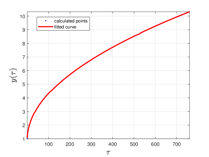
Refer to caption
(a)
Refer to caption
(b)
Refer to caption
(c)
Figure 3: Results on calculations: a) The temperature profile as a function of the time τ\tau and distance xx, the dashed line corresponds to T⁡(τ,x)=TmT(\tau,x)=T_{m}; (b) The law of the interphase boundary movement y⁡(τ)y(\tau); c) Jump in the gradient of temperature at the interphase boundary.

4 Conclusions

In this paper, we present another approach to solving various MHE problems, which can be viewed as an alternative to the method described in (Itkin et al. 2021b). This approach exploits the series expansion of the Dirac delta function into eigenfunctions of the corresponding Sturm-Liouville problem. We construct some new (oscillating) integral transforms and use them to solve several multilayer problems occurring in physics, finance, and biology. The number of such problems in science and engineering is vast.

The advantage of our method lies in the fact that our solutions are semi-analytical. This means that the answer is represented explicitly (perhaps, via some integrals). These integrals, however, depend on few yet unknown functions that solve a system of linear Volterra integral equations of the second kind. We derive this system in the paper and emphasize that, in general, it has to be solved numerically. However, as is shown in detail in (Itkin et al. 2021a), the corresponding numerical procedures are very efficient. In particular, they provide better speed and accuracy than the standard finite-difference (FD) methods.

Our main contribution to the existing literature lies in the fact that we consider moving boundaries, depending on time, while still constructing a semi-analytical solution. All previous approaches to these problems are purely numerical and rely on finite differences, finite elements, and similar methods. But, again, the semi-analytical solution has the advantage that the most challenging part of the problem is solved analytically, and the remaining part is solved numerically but with high efficiency.

As we mentioned earlier in the paper, various time-dependent problems with constant boundaries can be reduced to the MHE (or even to the Multilayer Bessel equations, (Decamps et al.)) by a set of transformations. However, as a result, the boundaries become time-dependent in the new variables. Therefore, our setting covers a broader class of problems than what the title claims.

For financial applications, this semi-analytical form is also very convenient to compute sensitivities of asset prices to various parameters of the model; see a thorough discussion in (Itkin et al. 2021a).

For physical and biological problems, the following comment is in order. This paper considers matching conditions at the layer boundaries (internal interfaces), which are the continuity of the solution and its flux over the boundary. As discussed in the literature, see, e.g., in (Hickson et al.), depending on what kind of physics problem is considered, various conditions at the internal interface can be set. It is possible to distinguish at least three different sets of matching conditions of particular interest. The first one assumes the temperature and flux continuity at the interfaces; we use it throughout this paper. The second matching condition deals with the conductivities, kik_{i}, as opposed to the diffusivities, and reads

ki​∂ui∂x|xi=ki+1​∂ui+1∂x|xi\left.k_{i}\frac{\partial u_{i}}{\partial x}\right|_{x_{i}}=\left.k_{i+1}\frac{\partial u_{i+1}}{\partial x}\right|_{x_{i}}

where ki=ρi​ci​κik_{i}=\rho_{i}c_{i}\kappa_{i}. This equation is more general than the continuity of the flux. It is applicable when the density, ρi\rho_{i}, and specific heat capacity cic_{i} are possibly different in each layer. The continuities of the flux and conductivities highlight the key difference between heat and mass transfer problems, as the former expresses the equality of the mass flux and the latter of the heat flux.

The third matching condition assumes a jump either in the solution or its flux (or both) at the interface (especially if this is a phase interface). Accordingly, it can be written in the form

κi​∂ui∂x\displaystyle\kappa_{i}\frac{\partial u_{i}}{\partial x} =Hi​(ui+1−ui),\displaystyle=H_{i}\left(u_{i+1}-u_{i}\right),
κi+1​∂ui+1∂x\displaystyle\kappa_{i+1}\frac{\partial u_{i+1}}{\partial x} =Hi+1​(ui+1−ui),\displaystyle=H_{i+1}\left(u_{i+1}-u_{i}\right),

where HiH_{i} is the contact transfer coefficient. This matching condition is more general than the previous ones as it models the roughness of the contact between the layers and contact resistance at the interfaces, see (Hickson et al.; Illingworth and Golosnoy). If Hi→∞H_{i}\rightarrow\infty, then the contact is perfect, and hence this limit represents the equivalent matching conditions from the previous cases. In a similar way the jump in the function value uu at the interface is often modeled by the condition ui​(τ,yi​(τ))=Pi​ui+1​(τ,yi​(τ))u_{i}(\tau,y_{i}(\tau))=P_{i}u_{i+1}(\tau,y_{i}(\tau)) where PIP_{I} is the partitioning coefficient which could be set constant or, in a more general case, is a function of time.

As far as our approach is concerned, it can deal with the second and third kinds of interface conditions. The integral transforms are the same, but solutions for the direct and inverse transforms are different. They rely on expanding discontinues functions into the Fourier series, which is possible and works fine. A detailed description of our method will be published elsewhere.

Another extension of the problem under consideration stems from choosing the boundary conditions at the external boundary. Usually, various analytical and semi-analytical solutions are constructed for the infinite or semi-infinite spatial domain. However, in real problems, e.g., that one discussed in (Illingworth and Golosnoy) and dedicated to finding transient solutions to diffusion problems in two distinct phases separated by a moving boundary, such an assumption is not valid. Indeed, in addition to ignoring the actual boundary conditions at the boundary walls, analytical methods have to assume that one of the phases has zero initial size. 88 8 We note that, in planar geometries, the exact solution can admittedly be extended to cover the case when both phases are initially non-zero. Such highly restrictive conditions mean that it is not possible to construct an analytical model for many situations, which are of considerable practical or industrial importance. However, for our method, these conditions are not as restrictive. Again, a detailed consideration will be presented elsewhere.

Acknowledgments

We thank Peter Carr who drew our attention to the book (Antimirov et al.), as well as for various fruitful discussions. Dmitry Muravey acknowledges support by the Russian Science Foundation under the Grant number 20-68-47030.

References

  • (1) D. Andreucci, E.N.M. Cirillo, M. Colangeli, and D. Gabrielli. Fick and Fokker-Planck Diffusion Law in Inhomogeneous Media. 174:469–493.
  • (2) S. Ankirchner, C Blanchet-Scalliet, and M. Jeanblanc. Controlling the occupation time of an exponential martingale. 70(2):415–428.
  • Ankirchner et al. (2021) S. Ankirchner, C. Blanchet-Scalliet, D. Dorobantu, and L. Gay. First passage time density of an Ornstein-Uhlenbeck process with broken drift. working paper, March 2021. URL https://hal.archives-ouvertes.fr/hal-03159498.
  • (4) M.Ya. Antimirov, A.A. Kolyshkin, and R. Vaillancourt. Applied integral transforms, volume 2. American Mathematical Society, reprint edition edition. ISBN 978-0821843147.
  • Asvestas et al. (2014) M Asvestas, A.G Sifalakis, E.P Papadopoulou, and Y.G Saridakis. Fokas method for a multi-domain linear reaction-diffusion equation with discontinuous diffusivity. Journal of Physics: Conference Series, 490(012143), 2014.
  • Carr and March (2018) E.J. Carr and N.G. March. Semi-analytical solution of multilayer diffusion problems with time-varying boundary conditions and general interface conditions. Applied Mathematics and Computation, 333(15):286–303, 2018.
  • (7) M. Decamps, M. Goovaerts, and W. Schoutens. Asymmetric skew Bessel processes and their applications to finance. 186(1):130–147.
  • Deconinck et al. (2014) B. Deconinck, T. Trogdon, and V. Vasan. The method of Fokas for solving linear partial differential equations. SIAM Review, 56(1):159–186, 2014.
  • Deconinck et al. (2016) B. Deconinck, B. Pelloni, B N.E., and NE Sheils. Non-steady-state heat conduction in composite walls. Proc. R. Soc. A, 470(20130605), 2016.
  • (10) P. Friz, P. Pigato, and J. Seibel. The step stochastic volatility model (ssvm). URL https://papers.ssrn.com/sol3/papers.cfm?abstract_id=3595408. SSRN: 3595408.
  • (11) A. Gairat and V. Shcherbakov. Density of Skew Brownian motionand its functionals with application in finance. 26(4):1069–1088.
  • (12) M. Goovaerts, M. Decamps, and W. Schoutens. Self exciting threshold interest rates models. 9(7):1093–1122.
  • Gradshtein and Ryzhik (2007) I.S. Gradshtein and I.M. Ryzhik. Table of Integrals, Series, and Products. Elsevier, 2007.
  • (14) Je-Chin Han. Analytical heat transfer. CRC Press, Boca Raton, FL. ISBN 978-1-4398-6196-7.
  • (15) R.I. Hickson, S.I. Barry, G.N. Mercer, and H.S. Sidhua. Finite difference schemes for multilayer diffusion. 54(1-2):210–220.
  • (16) T.C. Illingworth and I.O. Golosnoy. Numerical solutions of diffusion-controlled moving boundary problems which conserve solute. 209:207–225.
  • Itkin and Lipton (2018) A. Itkin and A. Lipton. Filling the gaps smoothly. Journal of Computational Sciences, 24:195–208, 2018.
  • Itkin and Muravey (2021) A. Itkin and D. Muravey. Semi-analytic pricing of double barrier options with time-dependent barriers and rebates at hit. Frontiers of Mathematical Finance, 1:1–36, 2021.
  • Itkin et al. (2021a) A. Itkin, A. Lipton, and D. Muravey. Generalized Integral Transforms in Mathematical Finance. WSPC, Singapore, 2021a. ISBN 978-981-123-173-5.
  • Itkin et al. (2021b) A. Itkin, A. Lipton, and D. Muravey. Multilayer heat equations: application to finance. 1, 2021b.
  • (21) K. Ito and H.P Jr. McKean. Diffusion Processes and their Sample Paths. Springer-Verlag Berlin Heidelberg. ISBN 978-3-642-62025-6.
  • (22) L.M. Jiji. Heat Conduction. Springer-Verlag, Berlin Heidelberg, 3rd edition. ISBN 978-3-642-01266-2.
  • (23) J.H. Keenan. Steam tables : thermodynamic properties of water including vapor, liquid, and solid phases. New York, 2nd edition. ISBN 0471042102.
  • (24) J. Keilson and J.A. Wellner. Oscillating Brownian motion. 15(2):300–310.
  • Lee (2002) Roger W. Lee. Implied volatility: Statics, dynamics, and probabilistic interpretation,. Discussion paper, Department of Mathematics, Stanford University, 2002.
  • Lejay (2006) A. Lejay. On the constructions of the skew Brownian motion. Probability Surveys, 3:413–466, 2006.
  • (27) A. Lejay and P. Pigato. A threshold model for local volatility : evidence of leverage and mean reversion effects on historical data. 22(4):1–24.
  • Lejay and Pigato (2018) A. Lejay and P. Pigato. Statistical estimation of the oscillating Brownian Motion. Bernoulli, 24(4B):3568 – 3602, 2018.
  • Lipton (2018) A. Lipton. Financial Engineering: Selected Works of Alexander Lipton. World Scientific, Singapore, 2018.
  • Lipton and Sepp (2011) A. Lipton and A. Sepp. Filling the gaps. Risk Magazine, pages 66–71, 2011.
  • (31) A. Lipton, A. Gal, and A. Lasis. Pricing of vanilla and first-generation exotic options in the local stochastic volatility framework: survey and new results. 14(11):1899–1922.
  • Mordecki and Salminen (2019) E. Mordecki and P. Salminen. Optimal stopping of Brownian motion with broken drift. High Frequency, 2(2):113–120, 2019.
  • Mumford et al. (1983) D. Mumford, C. Musiliand M. Nori, E. Previato, and M. Stillman. Tata Lectures on Theta. Progress in Mathematics. Birkhäuser Boston, 1983. ISBN 9780817631093.
  • Ohyama (1995) Y. Ohyama. Differential relations of theta functions. Osaka Journal of Mathematics, 32(2):431–450, 1995.
  • (35) P. Pigato. Extreme at-the-money skew in a local volatility model. 23:827–859.
  • Pontrelli et al. (2016) G. Pontrelli, M. Lauricella, J.A. Ferreira, and G. Pena. Iontophoretic transdermal drug delivery: A multi-layered approach. Mathematical Medicine and Biology, 00:1–18, 2016.
  • Ramirez et al. (2013) J.M. Ramirez, E.A. Thomann, and E.C. Waymire. Advection-dispersion across interfaces. Statistical Science, 28:487–509, 2013.
  • Salminen and Stenlund (2021) P. Salminen and D. Stenlund. Journal of Theoretical Probability, (2):975–1011, 2021.
  • (39) F. Sattin. Fick’s law and Fokker-Planck Equation in inhomogeneous environments. 172(22):3941–3945.
  • (40) A. Stetz. A beautiful theory: the relationship between beauty and scientific truth. URL http://sites.science.oregonstate.edu/˜stetza/ph407H/ABeautifulTheory.pdf.
  • (41) E.C. Titchmarsh. Eigenfunction Expansions Associated with Second-order Differential Equations. Oxford University Press, 2 edition. ISBN 978-0198533177.
  • (42) N.B. Vargaftik. Tables on the Thermophysical Properties of Liquids and Gases. Halsted Press, Division of John Wiley & Sons, Inc., New York.

Appendix A The expansion of the Dirac delta function for the continuous spectrum

Let us seek for the unknown function uλ​(x|x0)u_{\lambda}(x|x_{0}) to be in the form

uλ​(x|x0)\displaystyle u_{\lambda}(x|x_{0}) =𝟙x|y⊤​[A−​e−λ~−​(x−y)+12​σ−​λ​e−λ~−​|x−x0|A+​e−λ~+​(x−y)+12​σ+​λ​e−λ~+​|x−x0|,]\displaystyle=\bm{\mathbbm{1}}_{x|y}^{\top}\begin{bmatrix}A_{-}e^{-\tilde{\lambda}_{-}(x-y)}+\frac{1}{2\sigma_{-}\sqrt{\lambda}}e^{-\tilde{\lambda}_{-}|x-x_{0}|}\\ A_{+}e^{-\tilde{\lambda}_{+}(x-y)}+\frac{1}{2\sigma_{+}\sqrt{\lambda}}e^{-\tilde{\lambda}_{+}|x-x_{0}|},\end{bmatrix} (A.1)

where functions A±A_{\pm} are chosen to satisfy the matching conditions Eq. (20). In more detail, we need

limx→y±0uλ\displaystyle\lim_{x\to y\pm 0}u_{\lambda} =A±+12​σ±​λ​e−λ~±​|y−x0|,\displaystyle=A_{\pm}+\frac{1}{2\sigma_{\pm}\sqrt{\lambda}}e^{-\tilde{\lambda}_{\pm}|y-x_{0}|},
limx→y±0uλ,x\displaystyle\lim_{x\to y\pm 0}u_{\lambda,x} =λ~±​[∓A±+12​σ±​λ​e−λ~±​|y−x0|​(𝟙x0>y+𝟙x0<y)].\displaystyle=\tilde{\lambda}_{\pm}\left[\mp A_{\pm}+\frac{1}{2\sigma_{\pm}\sqrt{\lambda}}e^{-\tilde{\lambda}_{\pm}|y-x_{0}|}\left(\mathbbm{1}_{x_{0}>y}+\mathbbm{1}_{x_{0}<y}\right)\right].

Combining these two equations yields a linear system of equations for A−A_{-} and A+A_{+}

[1−1σ−σ+]​[A−A+]=12​λ​[1σ+​e−λ~+​|y−x0|−1σ−​e−λ~−​|y−x0|e−λ~+​|y−x0|​(𝟙x0>y−𝟙x0<y)−e−λ~−​|y−x0|​(𝟙x0>y−𝟙x0<y),]\displaystyle\begin{bmatrix}1&-1\\ \sigma_{-}&\sigma_{+}\end{bmatrix}\begin{bmatrix}A_{-}\\ A_{+}\end{bmatrix}=\frac{1}{2\sqrt{\lambda}}\begin{bmatrix}\frac{1}{\sigma_{+}}e^{-\tilde{\lambda}_{+}|y-x_{0}|}-\frac{1}{\sigma_{-}}e^{-\tilde{\lambda}_{-}|y-x_{0}|}\\ e^{-\tilde{\lambda}_{+}|y-x_{0}|}\left(\mathbbm{1}_{x_{0}>y}-\mathbbm{1}_{x_{0}<y}\right)-e^{-\tilde{\lambda}_{-}|y-x_{0}|}\left(\mathbbm{1}_{x_{0}>y}-\mathbbm{1}_{x_{0}<y}\right),\end{bmatrix}

with the following solution

[A−A+]\displaystyle\begin{bmatrix}A_{-}\\ A_{+}\end{bmatrix} =[Σ​e−λ~−​|x0−y|2​σ−​λ2​σ+σ−+σ+​e−λ~+​|x0−y|2​σ+​λ−e−λ~−​|x0−y|2​σ−​λ−e−λ~+​|x0−y|2​σ+​λ+2​σ−σ−+σ+​e−λ~−​|x0−y|2​σ−​λ−Σ​e−λ~+​|x0−y|2​σ+​λ]​𝟙x0|y,\displaystyle=\begin{bmatrix}\Sigma\frac{e^{-\tilde{\lambda}_{-}|x_{0}-y|}}{2\sigma_{-}\sqrt{\lambda}}&\frac{2\sigma_{+}}{\sigma_{-}+\sigma_{+}}\frac{e^{-\tilde{\lambda}_{+}|x_{0}-y|}}{2\sigma_{+}\sqrt{\lambda}}-\frac{e^{-\tilde{\lambda}_{-}|x_{0}-y|}}{2\sigma_{-}\sqrt{\lambda}}\\ -\frac{e^{-\tilde{\lambda}_{+}|x_{0}-y|}}{2\sigma_{+}\sqrt{\lambda}}+\frac{2\sigma_{-}}{\sigma_{-}+\sigma_{+}}\frac{e^{-\tilde{\lambda}_{-}|x_{0}-y|}}{2\sigma_{-}\sqrt{\lambda}}&-\Sigma\frac{e^{-\tilde{\lambda}_{+}|x_{0}-y|}}{2\sigma_{+}\sqrt{\lambda}}\end{bmatrix}\bm{\mathbbm{1}}_{x_{0}|y}, (A.2)
Σ\displaystyle\Sigma =σ−−σ+σ−+σ+.\displaystyle=\frac{\sigma_{-}-\sigma_{+}}{\sigma_{-}+\sigma_{+}}.

Accordingly, the function uλ​(x|x0)u_{\lambda}(x|x_{0}) can be represented as

uλ​(x|x0)=[𝟙x<y​e−λ~−​|x−y|𝟙x>y​e−λ~+​|x−y|]⊤​[A−A+]+𝟙x|y⊤​[e−λ~−​|x−x0|2​σ−​λe−λ~−​|x−x0|2​σ−​λe−λ~+​|x−x0|2​σ+​λe−λ~+​|x−x0|2​σ+​λ]​𝟙x0|y.\displaystyle u_{\lambda}(x|x_{0})=\begin{bmatrix}\mathbbm{1}_{x<y}e^{-\tilde{\lambda}_{-}|x-y|}\\ \mathbbm{1}_{x>y}e^{-\tilde{\lambda}_{+}|x-y|}\end{bmatrix}^{\top}\begin{bmatrix}A_{-}\\ A_{+}\end{bmatrix}+\bm{\mathbbm{1}}_{x|y}^{\top}\begin{bmatrix}\frac{e^{-\tilde{\lambda}_{-}|x-x_{0}|}}{2\sigma_{-}\sqrt{\lambda}}&\frac{e^{-\tilde{\lambda}_{-}|x-x_{0}|}}{2\sigma_{-}\sqrt{\lambda}}\\ \frac{e^{-\tilde{\lambda}_{+}|x-x_{0}|}}{2\sigma_{+}\sqrt{\lambda}}&\frac{e^{-\tilde{\lambda}_{+}|x-x_{0}|}}{2\sigma_{+}\sqrt{\lambda}}\end{bmatrix}\bm{\mathbbm{1}}_{x_{0}|y}. (A.3)

Re⁡λ\operatorname{Re}\lambdaIm⁡λ\operatorname{Im}\lambdaγ\gamma00γε\gamma_{\varepsilon}∙\bulletΓ+\Gamma_{+}Γ−\Gamma_{-}l1:λ=i​ωl_{1}:\sqrt{\lambda}=\mathrm{i}\mkern 1.0mu\omegal2:λ=−i​ωl_{2}:\sqrt{\lambda}=-\mathrm{i}\mkern 1.0mu\omega

Figure 4: Contours of integration in a complex plane in case of the continuous spectrum.

Now we are can compute the integral in Eq. (17). Let us extend the original contour (γ,−i​∞)−(γ,i​∞)(\gamma,-\mathrm{i}\mkern 1.0mu\infty)-(\gamma,\mathrm{i}\mkern 1.0mu\infty) to the loop contour LL in Fig. 4 which can be described as follows. It starts with a parallel line (γ,−i​R)−(γ,i​R)(\gamma,-\mathrm{i}\mkern 1.0muR)-(\gamma,\mathrm{i}\mkern 1.0muR), extending to a big symmetric arcs Γ−\Gamma_{-} and Γ+\Gamma_{+} around the point (γ,0)(\gamma,0) with the radius RR with the two horizontal line segments l1,l2l_{1},l_{2} connecting to a small circle γε\gamma_{\varepsilon} around the origin with the radius ε\varepsilon.

Using a standard technique, we take a limit ε→0,R→∞\varepsilon\to 0,R\to\infty, apply the Cauchy Residue theorem and obtain

∮Luλ​(x|x0)​𝑑λ=0.\oint_{L}u_{\lambda}(x|x_{0})d\lambda=0. (A.4)

Therefore,

δ⁡(x−x0)=12​π​i​∫γ−i​∞γ+i​∞uλ​(x|x0)​𝑑λ=∫0∞ue−i​π​ω2​(x|x0)−uei​π​ω2​(x|x0)π​i​ω​𝑑ω.\delta(x-x_{0})=\frac{1}{2\pi\mathrm{i}\mkern 1.0mu}\int_{\gamma-\mathrm{i}\mkern 1.0mu\infty}^{\gamma+\mathrm{i}\mkern 1.0mu\infty}u_{\lambda}(x|x_{0})d\lambda=\int_{0}^{\infty}\frac{u_{e^{-\mathrm{i}\mkern 1.0mu\pi}\omega^{2}}(x|x_{0})-u_{e^{\mathrm{i}\mkern 1.0mu\pi}\omega^{2}}(x|x_{0})}{\pi\mathrm{i}\mkern 1.0mu}\omega d\omega. (A.5)

Omitting tedious algebra, we find the following representation of the Dirac delta function

δ⁡(x−x0)\displaystyle\delta(x-x_{0}) =12​π​∫−∞+∞[ei​ω​x−yσ−σ−​𝟙x<yei​ω​x−yσ+σ+​𝟙x>y]⊤​[1+Σ​e2​i​ω​x0−yσ−1+Σ1−Σ1−Σ​e2​i​ω​x0−yσ+]​[e−i​ω​x0−yσ−​𝟙x0<ye−i​ω​x0−yσ+​𝟙x0>y]​𝑑ω.\displaystyle=\frac{1}{2\pi}\int_{-\infty}^{+\infty}\begin{bmatrix}\frac{e^{\mathrm{i}\mkern 1.0mu\omega\frac{x-y}{\sigma_{-}}}}{\sigma_{-}}\mathbbm{1}_{x<y}\\ \frac{e^{\mathrm{i}\mkern 1.0mu\omega\frac{x-y}{\sigma_{+}}}}{\sigma_{+}}\mathbbm{1}_{x>y}\end{bmatrix}^{\top}\begin{bmatrix}1+\Sigma e^{2\mathrm{i}\mkern 1.0mu\omega\frac{x_{0}-y}{\sigma_{-}}}&1+\Sigma\\ 1-\Sigma&1-\Sigma e^{2\mathrm{i}\mkern 1.0mu\omega\frac{x_{0}-y}{\sigma_{+}}}\end{bmatrix}\begin{bmatrix}e^{-\mathrm{i}\mkern 1.0mu\omega\frac{x_{0}-y}{\sigma_{-}}}\mathbbm{1}_{x_{0}<y}\\ e^{-\mathrm{i}\mkern 1.0mu\omega\frac{x_{0}-y}{\sigma_{+}}}\mathbbm{1}_{x_{0}>y}\end{bmatrix}d\omega. (A.6)

We proceed with separation of the variables xx and x0x_{0} in Eq. (A.6). Introducing the matrices (i.e. Forward and Backward)

ℱz,𝝈​(ω)\displaystyle\mathcal{F}_{z,\bm{\sigma}}(\omega) =𝒮ei​ω​zσ−,ei​ω​zσ+=[ei​ω​zσ−00ei​ω​zσ+],\displaystyle=\mathcal{S}_{e^{\frac{\mathrm{i}\mkern 1.0mu\omega z}{\sigma_{-}}},e^{\frac{\mathrm{i}\mkern 1.0mu\omega z}{\sigma_{+}}}}=\begin{bmatrix}e^{\frac{\mathrm{i}\mkern 1.0mu\omega z}{\sigma_{-}}}&0\\ 0&e^{\frac{\mathrm{i}\mkern 1.0mu\omega z}{\sigma_{+}}}\end{bmatrix}, (A.7)
ℬz,𝝈​(ω)\displaystyle\mathcal{B}_{z,\bm{\sigma}}(\omega) =[1σ−​(e−i​ω​zσ−+Σ​ei​ω​zσ−)1σ−​(1+Σ)​e−i​ω​zσ+1σ+​(1−Σ)​e−i​ω​zσ−1σ+​(e−i​ω​zσ+−Σ​ei​ω​zσ+)],\displaystyle=\begin{bmatrix}\frac{1}{\sigma_{-}}\left(e^{-\frac{\mathrm{i}\mkern 1.0mu\omega z}{\sigma_{-}}}+\Sigma e^{\frac{\mathrm{i}\mkern 1.0mu\omega z}{\sigma_{-}}}\right)&\frac{1}{\sigma_{-}}\left(1+\Sigma\right)e^{-\frac{\mathrm{i}\mkern 1.0mu\omega z}{\sigma_{+}}}\\ \frac{1}{\sigma_{+}}\left(1-\Sigma\right)e^{-\frac{\mathrm{i}\mkern 1.0mu\omega z}{\sigma_{-}}}&\frac{1}{\sigma_{+}}\left(e^{-\frac{\mathrm{i}\mkern 1.0mu\omega z}{\sigma_{+}}}-\Sigma e^{\frac{\mathrm{i}\mkern 1.0mu\omega z}{\sigma_{+}}}\right)\end{bmatrix},

the Eq. (A.6) can be re-written as

δ⁡(x−x0)=12​π​∫−∞+∞𝟙x|y⊤​ℱx−y,𝝈​(ω)​ℬx0−y,𝝈​(ω)​𝟙x0|y​𝑑ω.\displaystyle\delta(x-x_{0})=\frac{1}{2\pi}\int_{-\infty}^{+\infty}\bm{\mathbbm{1}}_{x|y}^{\top}\mathcal{F}_{x-y,\bm{\sigma}}(\omega)\mathcal{B}_{x_{0}-y,\bm{\sigma}}(\omega)\bm{\mathbbm{1}}_{x_{0}|y}d\omega. (A.8)

It is worth mentioning that the matrix ℱx,y,𝝈\mathcal{F}_{x,y,\bm{\sigma}} has a semigroup property with respect to the matrix multiplication, i.e.

ℱz,𝝈​(ω)​ℱζ,𝝈​(ω)=ℱz+ζ,𝝈​(ω).\mathcal{F}_{z,\bm{\sigma}}(\omega)\mathcal{F}_{\zeta,\bm{\sigma}}(\omega)=\mathcal{F}_{z+\zeta,\bm{\sigma}}(\omega). (A.9)

Appendix B Contour integration

By analogy with computation of the integral in Eq. (17), we extend the contour (γ,−i​∞)−(γ,i​∞)(\gamma,-\mathrm{i}\mkern 1.0mu\infty)-(\gamma,\mathrm{i}\mkern 1.0mu\infty) to the loop contour LL shown in Fig. 5. However, in this case the integration domain contains simple poles which are determined by the equation det𝚲∗​(λ)=0\det\bm{\Lambda}^{*}(\lambda)=0. Again, we proceed in a way similar to that for Eq. (17), i.e., by taking a limit ε→0,R→∞\varepsilon\to 0,R\to\infty and applying the Cauchy Residue theorem. Omitting an intermediate algebra, we provide just the final result which is the representation in Eq. (59).

∙\bullet∙\bullet∙\bullet∙\bullet∙\bullet∙\bullet∙\bullet∙\bullet∙\bullet∙\bulletRe⁡λ\operatorname{Re}\lambdaIm⁡λ\operatorname{Im}\lambdaγ\gamma00γε\gamma_{\varepsilon}∙\bulletΓ+\Gamma_{+}Γ−\Gamma_{-}l1:λ=i​ωl_{1}:\sqrt{\lambda}=\mathrm{i}\mkern 1.0mu\omegal2:λ=−i​ωl_{2}:\sqrt{\lambda}=-\mathrm{i}\mkern 1.0mu\omega

Figure 5: Contours of integration in a complex plane in case of the mixed spectrum.

Appendix C Solution of Eq. (76)

To solve Eq. (76) we use the oscillating transform

𝒖¯​(τ,ω)=[u¯−​(τ,ω)u¯+​(τ,ω)]=∫−∞∞ℱx,𝝈​(ω)​𝟙x|y⁡(τ)​u​(τ,x)​𝑑x,\displaystyle\bm{\bar{u}}(\tau,\omega)=\begin{bmatrix}\bar{u}_{-}(\tau,\omega)\\ \bar{u}_{+}(\tau,\omega)\end{bmatrix}=\int_{-\infty}^{\infty}\mathcal{F}_{x,\bm{\sigma}}(\omega)\bm{\mathbbm{1}}_{x|y(\tau)}u(\tau,x)dx, (C.1)

where the matrix ℱx,𝝈​(ω)\mathcal{F}_{x,\bm{\sigma}}(\omega) was defined in Eq. (A.7). Using the semigroup property Eq. (A.9) in the inversion formula 28 yields

u⁡(τ,x)=12​π​∫−∞∞𝒖¯​(τ,ω)⊤​ℱ−y⁡(τ),𝝈​(ω)​ℬx−y⁡(τ),𝝈​(ω)​𝟙x|y⁡(τ)​𝑑ω.\displaystyle u(\tau,x)=\frac{1}{2\pi}\int_{-\infty}^{\infty}\bm{\bar{u}}(\tau,\omega)^{\top}\mathcal{F}_{-y(\tau),\bm{\sigma}}(\omega)\mathcal{B}_{x-y(\tau),\bm{\sigma}}(\omega)\bm{\mathbbm{1}}_{x|y(\tau)}d\omega. (C.2)

The images u¯−\bar{u}_{-} and u¯+\bar{u}_{+} can be easily found in the explicit form and read

u¯−​(τ,ω)=∫−∞y⁡(τ)ei​ω​xσ−​u​(τ,x)​𝑑x,u¯+​(τ,ω)=∫y⁡(τ)+∞ei​ω​xσ+​u​(τ,x)​𝑑x\displaystyle\bar{u}_{-}(\tau,\omega)=\int_{-\infty}^{y(\tau)}e^{\frac{\mathrm{i}\mkern 1.0mu\omega x}{\sigma_{-}}}u(\tau,x)dx,\qquad\bar{u}_{+}(\tau,\omega)=\int^{+\infty}_{y(\tau)}e^{\frac{\mathrm{i}\mkern 1.0mu\omega x}{\sigma_{+}}}u(\tau,x)dx (C.3)

To make these integrals well-behaved we need function u⁡(τ,x)u(\tau,x) to vanish at plus and minus infinity faster than the corresponding exponent99 9 Actually, as shown below integrals on ω\omega in Eq. (C.9) are regular, so there is no problem with convergence of these transforms.. Now we define new functions Φ⁡(τ),ϕ⁡(τ)\Phi(\tau),\phi(\tau) as

σ−2​∂u⁡(τ,x)∂x|x=y⁡(τ)−0=σ+2​∂u⁡(τ,x)∂x|x=y⁡(τ)+0=Φ⁡(τ),u⁡(τ,y⁡(τ))=φ⁡(τ),\sigma^{2}_{-}\frac{\partial u(\tau,x)}{\partial x}\bigg|_{x=y(\tau)-0}=\sigma^{2}_{+}\frac{\partial u(\tau,x)}{\partial x}\bigg|_{x=y(\tau)+0}=\Phi(\tau),\quad u(\tau,y(\tau))=\varphi(\tau), (C.4)

and apply the transform Eq. (C.1) directly to the both sides of the last line in Eq. (76)

∫−∞y⁡(τ)σ−2​ux​x​ei​ω​xσ−​𝑑x\displaystyle\int_{-\infty}^{y(\tau)}\sigma_{-}^{2}u_{xx}e^{\frac{\mathrm{i}\mkern 1.0mu\omega x}{\sigma_{-}}}dx =ei​ω​y​(τ)σ−​Φ​(τ)−i​ω​σ−​∫−∞y⁡(τ)ux​ei​ω​xσ−​𝑑x\displaystyle=e^{\frac{\mathrm{i}\mkern 1.0mu\omega y(\tau)}{\sigma_{-}}}\Phi(\tau)-\mathrm{i}\mkern 1.0mu\omega\sigma_{-}\int_{-\infty}^{y(\tau)}u_{x}e^{\frac{\mathrm{i}\mkern 1.0mu\omega x}{\sigma_{-}}}dx
=ei​ω​y​(τ)σ−​Φ​(τ)−i​ω​σ−​ei​ω​y​(τ)σ−​φ​(τ)−ω2​u¯−​(τ,ω),\displaystyle=e^{\frac{\mathrm{i}\mkern 1.0mu\omega y(\tau)}{\sigma_{-}}}\Phi(\tau)-\mathrm{i}\mkern 1.0mu\omega\sigma_{-}e^{\frac{\mathrm{i}\mkern 1.0mu\omega y(\tau)}{\sigma_{-}}}\varphi(\tau)-\omega^{2}\bar{u}_{-}(\tau,\omega),
∫−∞y⁡(τ)uτ​ei​ω​xσ−​𝑑x\displaystyle\int_{-\infty}^{y(\tau)}u_{\tau}e^{\frac{\mathrm{i}\mkern 1.0mu\omega x}{\sigma_{-}}}dx =∂∂τ​∫−∞y⁡(τ)ei​ω​xσ−​u​(τ,x)​𝑑x−y′​(τ)​ei​ω​y​(τ)σ−​u​(τ,y⁡(τ))=∂u¯−∂τ−y′​(τ)​ei​ω​y​(τ)σ−​ϕ​(τ),\displaystyle=\frac{\partial}{\partial\tau}\int_{-\infty}^{y(\tau)}e^{\frac{\mathrm{i}\mkern 1.0mu\omega x}{\sigma_{-}}}u(\tau,x)dx-y^{\prime}(\tau)e^{\frac{\mathrm{i}\mkern 1.0mu\omega y(\tau)}{\sigma_{-}}}u(\tau,y(\tau))=\frac{\partial\bar{u}_{-}}{\partial\tau}-y^{\prime}(\tau)e^{\frac{\mathrm{i}\mkern 1.0mu\omega y(\tau)}{\sigma_{-}}}\phi(\tau),
∫y⁡(τ)+∞σ+2​ux​x​ei​ω​xσ+​𝑑x\displaystyle\int^{+\infty}_{y(\tau)}\sigma_{+}^{2}u_{xx}e^{\frac{\mathrm{i}\mkern 1.0mu\omega x}{\sigma_{+}}}dx =−ei​ω​y​(τ)σ+​Φ​(τ)−i​ω​σ+​∫y⁡(τ)+∞ux​ei​ω​xσ+​𝑑x\displaystyle=-e^{\frac{\mathrm{i}\mkern 1.0mu\omega y(\tau)}{\sigma_{+}}}\Phi(\tau)-\mathrm{i}\mkern 1.0mu\omega\sigma_{+}\int^{+\infty}_{y(\tau)}u_{x}e^{\frac{\mathrm{i}\mkern 1.0mu\omega x}{\sigma_{+}}}dx
=−ei​ω​y​(τ)σ+​Φ​(τ)+i​ω​σ+​ei​ω​y​(τ)σ+​φ​(τ)−ω2​u¯+​(τ,ω),\displaystyle=-e^{\frac{\mathrm{i}\mkern 1.0mu\omega y(\tau)}{\sigma_{+}}}\Phi(\tau)+\mathrm{i}\mkern 1.0mu\omega\sigma_{+}e^{\frac{\mathrm{i}\mkern 1.0mu\omega y(\tau)}{\sigma_{+}}}\varphi(\tau)-\omega^{2}\bar{u}_{+}(\tau,\omega),
∫y⁡(τ)+∞uτ​ei​ω​xσ+​𝑑x\displaystyle\int^{+\infty}_{y(\tau)}u_{\tau}e^{\frac{\mathrm{i}\mkern 1.0mu\omega x}{\sigma_{+}}}dx =∂∂τ​∫y⁡(τ)+∞ei​ω​xσ+​u​(τ,x)​𝑑x+y′​(τ)​ei​ω​y​(τ)σ+​u​(τ,y⁡(τ))=∂u¯+∂τ+y′​(τ)​ei​ω​y​(τ)σ+​ϕ​(τ).\displaystyle=\frac{\partial}{\partial\tau}\int^{+\infty}_{y(\tau)}e^{\frac{\mathrm{i}\mkern 1.0mu\omega x}{\sigma_{+}}}u(\tau,x)dx+y^{\prime}(\tau)e^{\frac{\mathrm{i}\mkern 1.0mu\omega y(\tau)}{\sigma_{+}}}u(\tau,y(\tau))=\frac{\partial\bar{u}_{+}}{\partial\tau}+y^{\prime}(\tau)e^{\frac{\mathrm{i}\mkern 1.0mu\omega y(\tau)}{\sigma_{+}}}\phi(\tau).

Therefore, the matching conditions in Eq. (76) give rise to two independent ordinary differential equations (ODE) (with respect to τ\tau)

∂u¯−∂τ+ω2​u¯−\displaystyle\frac{\partial\bar{u}_{-}}{\partial\tau}+\omega^{2}\bar{u}_{-} =ei​ω​y​(τ)σ−​Φ​(τ)−i​ω​σ−​ei​ω​y​(τ)σ−​φ​(τ)+y′​(τ)​ei​ω​y​(τ)σ−​ϕ​(τ),u¯−​(0,ω)=𝟙x0<y⁡(0)​ei​ω​x0σ−,\displaystyle=e^{\frac{\mathrm{i}\mkern 1.0mu\omega y(\tau)}{\sigma_{-}}}\Phi(\tau)-\mathrm{i}\mkern 1.0mu\omega\sigma_{-}e^{\frac{\mathrm{i}\mkern 1.0mu\omega y(\tau)}{\sigma_{-}}}\varphi(\tau)+y^{\prime}(\tau)e^{\frac{\mathrm{i}\mkern 1.0mu\omega y(\tau)}{\sigma_{-}}}\phi(\tau),\quad\bar{u}_{-}(0,\omega)=\mathbbm{1}_{x_{0}<y(0)}e^{\frac{\mathrm{i}\mkern 1.0mu\omega x_{0}}{\sigma_{-}}},
∂u¯+∂τ+ω2​u¯+\displaystyle\frac{\partial\bar{u}_{+}}{\partial\tau}+\omega^{2}\bar{u}_{+} =−ei​ω​y​(τ)σ+​Φ​(τ)+i​ω​σ+​ei​ω​y​(τ)σ+​φ​(τ)−y′​(τ)​ei​ω​y​(τ)σ+​ϕ​(τ),u¯+​(0,ω)=𝟙x0>y⁡(0)​ei​ω​x0σ+.\displaystyle=-e^{\frac{\mathrm{i}\mkern 1.0mu\omega y(\tau)}{\sigma_{+}}}\Phi(\tau)+\mathrm{i}\mkern 1.0mu\omega\sigma_{+}e^{\frac{\mathrm{i}\mkern 1.0mu\omega y(\tau)}{\sigma_{+}}}\varphi(\tau)-y^{\prime}(\tau)e^{\frac{\mathrm{i}\mkern 1.0mu\omega y(\tau)}{\sigma_{+}}}\phi(\tau),\quad\bar{u}_{+}(0,\omega)=\mathbbm{1}_{x_{0}>y(0)}e^{\frac{\mathrm{i}\mkern 1.0mu\omega x_{0}}{\sigma_{+}}}.

These equations can be solved analytically via a standard technique

u¯−​(τ,ω)\displaystyle\bar{u}_{-}(\tau,\omega) =𝟙x0<y⁡(0)​e−ω2​τ+i​ω​x0σ−\displaystyle=\mathbbm{1}_{x_{0}<y(0)}e^{-\omega^{2}\tau+\mathrm{i}\mkern 1.0mu\omega\frac{x_{0}}{\sigma_{-}}} (C.5)
+∫0τe−ω2​(τ−s)[ei​ω​y​(s)σ−Φ(s)−iωσ−ei​ω​y​(s)σ−φ(s)+y′(s)ei​ω​y​(s)σ−φ(s)]ds,\displaystyle+\int_{0}^{\tau}e^{-\omega^{2}(\tau-s)}\left[e^{\frac{\mathrm{i}\mkern 1.0mu\omega y(s)}{\sigma_{-}}}\Phi(s)-\mathrm{i}\mkern 1.0mu\omega\sigma_{-}e^{\frac{\mathrm{i}\mkern 1.0mu\omega y(s)}{\sigma_{-}}}\varphi(s)+y^{\prime}(s)e^{\frac{\mathrm{i}\mkern 1.0mu\omega y(s)}{\sigma_{-}}}\varphi(s)\right]ds,
u¯+​(τ,ω)\displaystyle\bar{u}_{+}(\tau,\omega) =𝟙x0>y⁡(0)​e−ω2​τ+i​ω​x0σ+\displaystyle=\mathbbm{1}_{x_{0}>y(0)}e^{-\omega^{2}\tau+\mathrm{i}\mkern 1.0mu\omega\frac{x_{0}}{\sigma_{+}}}
−∫0τe−ω2​(τ−s)[ei​ω​y​(s)σ+Φ(s)−iωσ+ei​ω​y​(s)σ+φ(s)+y′(s)ei​ω​y​(s)σ+φ(s)]ds.\displaystyle-\int_{0}^{\tau}e^{-\omega^{2}(\tau-s)}\left[e^{\frac{\mathrm{i}\mkern 1.0mu\omega y(s)}{\sigma_{+}}}\Phi(s)-\mathrm{i}\mkern 1.0mu\omega\sigma_{+}e^{\frac{\mathrm{i}\mkern 1.0mu\omega y(s)}{\sigma_{+}}}\varphi(s)+y^{\prime}(s)e^{\frac{\mathrm{i}\mkern 1.0mu\omega y(s)}{\sigma_{+}}}\varphi(s)\right]ds.

This result can be also expressed in the matrix form

𝒖¯​(τ,ω)\displaystyle\bm{\bar{u}}(\tau,\omega) =e−ω2​τ​ℱx0,𝝈​(ω)​𝟙x0|y⁡(0)+∫0τe−ω2​(τ−s)​ℱy⁡(s),𝝈​(ω)​[Φ⁡(s)−i​ω​σ−​φ​(s)+y′​(s)​φ​(s)−Φ⁡(s)+i​ω​σ+​φ​(s)−y′​(s)​φ​(s)]​𝑑s.\displaystyle=e^{-\omega^{2}\tau}\mathcal{F}_{x_{0},\bm{\sigma}}(\omega)\bm{\mathbbm{1}}_{x_{0}|y(0)}+\int_{0}^{\tau}e^{-\omega^{2}(\tau-s)}\mathcal{F}_{y(s),\bm{\sigma}}(\omega)\begin{bmatrix}\Phi(s)-\mathrm{i}\mkern 1.0mu\omega\sigma_{-}\varphi(s)+y^{\prime}(s)\varphi(s)\\ -\Phi(s)+\mathrm{i}\mkern 1.0mu\omega\sigma_{+}\varphi(s)-y^{\prime}(s)\varphi(s)\end{bmatrix}ds. (C.6)

Applying the inversion formula Eq. (C.2) we arrive at the following representation

u⁡(τ,x)\displaystyle u(\tau,x) =12​π​∫−∞∞e−ω2​τ​𝟙x0|y⁡(0)⊤​ℱx0−y⁡(τ),𝝈​(ω)​ℬx−y⁡(τ),𝝈​(ω)​𝟙x|y⁡(τ)​𝑑ω\displaystyle=\frac{1}{2\pi}\int_{-\infty}^{\infty}e^{-\omega^{2}\tau}\bm{\mathbbm{1}}_{x_{0}|y(0)}^{\top}\mathcal{F}_{x_{0}-y(\tau),\bm{\sigma}}(\omega)\mathcal{B}_{x-y(\tau),\bm{\sigma}}(\omega)\bm{\mathbbm{1}}_{x|y(\tau)}d\omega (C.7)
+12​π∫−∞∞∫0τe−ω2​(τ−s)𝚿(s,ω)⊤ℱy⁡(s)−y⁡(τ),𝝈(ω)ℬx−y⁡(τ),𝝈(ω)𝟙x|y⁡(τ)dsdω,\displaystyle+\frac{1}{2\pi}\int_{-\infty}^{\infty}\int_{0}^{\tau}e^{-\omega^{2}(\tau-s)}\bm{\Psi}(s,\omega)^{\top}\mathcal{F}_{y(s)-y(\tau),\bm{\sigma}}(\omega)\mathcal{B}_{x-y(\tau),\bm{\sigma}}(\omega)\bm{\mathbbm{1}}_{x|y(\tau)}dsd\omega,

where 𝚿⁡(s,ω)\bm{\Psi}(s,\omega) is defined as

𝚿⁡(s,ω)=[Φ⁡(s)+y′​(s)​φ​(s)]​[1−1]−i​ω​φ​(s)​[σ−00σ+]​[1−1].\bm{\Psi}(s,\omega)=\left[\Phi(s)+y^{\prime}(s)\varphi(s)\right]\begin{bmatrix}1\\ -1\end{bmatrix}-\mathrm{i}\mkern 1.0mu\omega\varphi(s)\begin{bmatrix}\sigma_{-}&0\\ 0&\sigma_{+}\end{bmatrix}\begin{bmatrix}1\\ -1\end{bmatrix}. (C.8)

The integrals with respect to ω\omega can be computed analytically. Indeed, using the identities, (Gradshtein and Ryzhik 2007)

12​π​∫−∞+∞e−ω2​(τ−s)+i​α​ω​𝑑ω=e−α24​(τ−s)2​π⁡(τ−s),12​π​∫−∞+∞i​ω​e−ω2​(τ−s)+i​α​ω​𝑑ω=−α​e−α24​(τ−s)4​π​(τ−s)3,\displaystyle\frac{1}{2\pi}\int_{-\infty}^{+\infty}e^{-\omega^{2}(\tau-s)+\mathrm{i}\mkern 1.0mu\alpha\omega}d\omega=\frac{e^{-\frac{\alpha^{2}}{4(\tau-s)}}}{2\sqrt{\pi(\tau-s)}},\qquad\frac{1}{2\pi}\int_{-\infty}^{+\infty}\mathrm{i}\mkern 1.0mu\omega e^{-\omega^{2}(\tau-s)+\mathrm{i}\mkern 1.0mu\alpha\omega}d\omega=-\frac{\alpha e^{-\frac{\alpha^{2}}{4(\tau-s)}}}{4\sqrt{\pi(\tau-s)^{3}}}, (C.9)

and the explicit formula for the matrix product ℱζ,𝝈​(ω)​ℬz,𝝈​(ω)\mathcal{F}_{\zeta,\bm{\sigma}}(\omega)\mathcal{B}_{z,\bm{\sigma}}(\omega)

ℱζ,𝝈​(ω)​ℬz,𝝈​(ω)\displaystyle\mathcal{F}_{\zeta,\bm{\sigma}}(\omega)\mathcal{B}_{z,\bm{\sigma}}(\omega) =[1σ−​ei​ω​ζσ−​(e−i​ω​zσ−+Σ​ei​ω​zσ−)1σ−​ei​ω​ζσ−​(1+Σ)​e−i​ω​zσ+1σ+​ei​ω​ζσ+​(1−Σ)​e−i​ω​zσ−1σ+​ei​ω​ζσ+​(e−i​ω​zσ+−Σ​ei​ω​zσ+)],Σ=σ−−σ+σ−+σ+.\displaystyle=\begin{bmatrix}\frac{1}{\sigma_{-}}e^{\frac{\mathrm{i}\mkern 1.0mu\omega\zeta}{\sigma_{-}}}\left(e^{-\frac{\mathrm{i}\mkern 1.0mu\omega z}{\sigma_{-}}}+\Sigma e^{\frac{\mathrm{i}\mkern 1.0mu\omega z}{\sigma_{-}}}\right)&\frac{1}{\sigma_{-}}e^{\frac{\mathrm{i}\mkern 1.0mu\omega\zeta}{\sigma_{-}}}\left(1+\Sigma\right)e^{-\frac{\mathrm{i}\mkern 1.0mu\omega z}{\sigma_{+}}}\\ \frac{1}{\sigma_{+}}e^{\frac{\mathrm{i}\mkern 1.0mu\omega\zeta}{\sigma_{+}}}\left(1-\Sigma\right)e^{-\frac{\mathrm{i}\mkern 1.0mu\omega z}{\sigma_{-}}}&\frac{1}{\sigma_{+}}e^{\frac{\mathrm{i}\mkern 1.0mu\omega\zeta}{\sigma_{+}}}\left(e^{-\frac{\mathrm{i}\mkern 1.0mu\omega z}{\sigma_{+}}}-\Sigma e^{\frac{\mathrm{i}\mkern 1.0mu\omega z}{\sigma_{+}}}\right)\\ \end{bmatrix},\qquad\Sigma=\frac{\sigma_{-}-\sigma_{+}}{\sigma_{-}+\sigma_{+}}.

yields

12​π∫−∞+∞\displaystyle\frac{1}{2\pi}\int_{-\infty}^{+\infty} e−ω2​(τ−s)​ωℱζ,𝝈(ω)ℬz,𝝈(ω)dω=𝒫𝝈(z,τ|ζ,s),\displaystyle e^{-\omega^{2}(\tau-s)\omega}\mathcal{F}_{\zeta,\bm{\sigma}}(\omega)\mathcal{B}_{z,\bm{\sigma}}(\omega)d\omega=\mathcal{P}_{\bm{\sigma}}(z,\tau|\zeta,s), (C.10)
12​π∫−∞+∞\displaystyle\frac{1}{2\pi}\int_{-\infty}^{+\infty} iωe−ω2​(τ−s)​ωℱζ,𝝈(ω)ℬz,𝝈(ω)dω=𝜼𝝈(z,τ|ζ,s),\displaystyle\mathrm{i}\mkern 1.0mu\omega e^{-\omega^{2}(\tau-s)\omega}\mathcal{F}_{\zeta,\bm{\sigma}}(\omega)\mathcal{B}_{z,\bm{\sigma}}(\omega)d\omega=\bm{\eta}_{\bm{\sigma}}(z,\tau|\zeta,s),
𝒫𝝈(z,τ|ζ,s)\displaystyle\mathcal{P}_{\bm{\sigma}}(z,\tau|\zeta,s) =12​π⁡(τ−s)​[1σ−001σ+]\displaystyle=\frac{1}{2\sqrt{\pi(\tau-s)}}\begin{bmatrix}\frac{1}{\sigma_{-}}&0\\ 0&\frac{1}{\sigma_{+}}\end{bmatrix}
×[e−(z−ζ)24​σ−2​(τ−s)+Σ​e−(z+ζ)24​σ−2​(τ−s)(1+Σ)​e−(z/σ+−ζ/σ−)24​(τ−s)(1−Σ)​e−(z/σ−−ζ/σ+)24​(τ−s)e−(z−ζ)24​σ+2​(τ−s)−Σ​e−(z+ζ)24​σ+2​(τ−s)],\displaystyle\times\begin{bmatrix}e^{-\frac{\left(z-\zeta\right)^{2}}{4\sigma_{-}^{2}(\tau-s)}}+\Sigma e^{-\frac{\left(z+\zeta\right)^{2}}{4\sigma_{-}^{2}(\tau-s)}}&\left(1+\Sigma\right)e^{-\frac{\left(z/\sigma_{+}-\zeta/\sigma_{-}\right)^{2}}{4(\tau-s)}}\\ \left(1-\Sigma\right)e^{-\frac{\left(z/\sigma_{-}-\zeta/\sigma_{+}\right)^{2}}{4(\tau-s)}}&e^{-\frac{\left(z-\zeta\right)^{2}}{4\sigma_{+}^{2}(\tau-s)}}-\Sigma e^{-\frac{\left(z+\zeta\right)^{2}}{4\sigma_{+}^{2}(\tau-s)}}\end{bmatrix},
𝜼𝝈(z,τ|ζ,s)\displaystyle\bm{\eta}_{\bm{\sigma}}(z,\tau|\zeta,s) =−14​π​(τ−s)3​[1σ−001σ+]\displaystyle=-\frac{1}{4\sqrt{\pi(\tau-s)^{3}}}\begin{bmatrix}\frac{1}{\sigma_{-}}&0\\ 0&\frac{1}{\sigma_{+}}\end{bmatrix}
×[ζ−zσ−​e−(z−ζ)24​σ−2​(τ−s)+ζ+zσ−​Σ​e−(z+ζ)24​σ−2​(τ−s)[ζσ−−zσ+]​(1+Σ)​e−(z/σ+−ζ/σ−)24​(τ−s)[ζσ+−zσ−]​(1−Σ)​e−(z/σ−−ζ/σ+)24​(τ−s)ζ−zσ+​e−(z−ζ)24​σ+2​(τ−s)−ζ+zσ+​Σ​e−(z+ζ)24​σ+2​(τ−s)].\displaystyle\times\begin{bmatrix}\frac{\zeta-z}{\sigma_{-}}e^{-\frac{\left(z-\zeta\right)^{2}}{4\sigma_{-}^{2}(\tau-s)}}+\frac{\zeta+z}{\sigma_{-}}\Sigma e^{-\frac{\left(z+\zeta\right)^{2}}{4\sigma_{-}^{2}(\tau-s)}}&\left[\frac{\zeta}{\sigma_{-}}-\frac{z}{\sigma_{+}}\right]\left(1+\Sigma\right)e^{-\frac{\left(z/\sigma_{+}-\zeta/\sigma_{-}\right)^{2}}{4(\tau-s)}}\\ \left[\frac{\zeta}{\sigma_{+}}-\frac{z}{\sigma_{-}}\right]\left(1-\Sigma\right)e^{-\frac{\left(z/\sigma_{-}-\zeta/\sigma_{+}\right)^{2}}{4(\tau-s)}}&\frac{\zeta-z}{\sigma_{+}}e^{-\frac{\left(z-\zeta\right)^{2}}{4\sigma_{+}^{2}(\tau-s)}}-\frac{\zeta+z}{\sigma_{+}}\Sigma e^{-\frac{\left(z+\zeta\right)^{2}}{4\sigma_{+}^{2}(\tau-s)}}\end{bmatrix}.

Therefore, u⁡(τ,x)u(\tau,x) reads

u⁡(τ,x)\displaystyle u(\tau,x) =⟨𝟙x0|y⁡(0),𝒫𝝈(x−y(τ),τ,|x0−y(τ),0)𝟙x|y⁡(τ)⟩\displaystyle=\left\langle\bm{\mathbbm{1}}_{x_{0}|y(0)},\mathcal{P}_{\bm{\sigma}}(x-y(\tau),\tau,|x_{0}-y(\tau),0)\bm{\mathbbm{1}}_{x|y(\tau)}\right\rangle (C.11)
+∫0τ[Φ(s)+y′(s)φ(s)]⟨[1−1],𝒫𝝈(x−y(τ),τ|y(s)−y(τ),s)𝟙x|y⁡(τ)⟩ds\displaystyle+\int_{0}^{\tau}\left[\Phi(s)+y^{\prime}(s)\varphi(s)\right]\left\langle\begin{bmatrix}1\\ -1\end{bmatrix},\mathcal{P}_{\bm{\sigma}}(x-y(\tau),\tau|y(s)-y(\tau),s)\bm{\mathbbm{1}}_{x|y(\tau)}\right\rangle ds
+∫0τφ(s)⟨[1−1],𝜼𝝈(x−y(τ),τ|y(s)−y(τ),s)𝟙x|y⁡(τ)⟩ds.\displaystyle+\int_{0}^{\tau}\varphi(s)\left\langle\begin{bmatrix}1\\ -1\end{bmatrix},\bm{\eta}_{\bm{\sigma}}(x-y(\tau),\tau|y(s)-y(\tau),s)\bm{\mathbbm{1}}_{x|y(\tau)}\right\rangle ds.

Appendix D Explicit representation of the inverse transform in Eq. (83)

An explicit representation of the inverse transform in Eq. (83) can be obtained if we know all its components u¯iC​(τ,λ),u¯iS​(τ,λ)\bar{u}^{C}_{i}(\tau,\lambda),\ \bar{u}^{S}_{i}(\tau,\lambda) defined in Eq. (84). Our main idea consists in finding them separately and then constructing the whole image u¯\bar{u} as a weighted sum. For doing so, let us denote the values of u⁡(τ,x)u(\tau,x) and their gradients at all internal interfaces between the layers as

∂u⁡(τ,x)∂x|x→yi−1​(τ)+0\displaystyle\frac{\partial u(\tau,x)}{\partial x}\Bigg|_{x\to y_{i-1}(\tau)+0} =Ψi−​(τ),\displaystyle=\Psi_{i}^{-}(\tau), ∂u⁡(τ,x)∂x|x→yi​(τ)−0\displaystyle\qquad\frac{\partial u(\tau,x)}{\partial x}\Bigg|_{x\to y_{i}(\tau)-0} =Ψi+​(τ),\displaystyle=\Psi_{i}^{+}(\tau), (D.1)
u⁡(τ,yi−1​(τ)+0)\displaystyle u(\tau,y_{i-1}(\tau)+0) =ϕi−​(τ),\displaystyle=\phi_{i}^{-}(\tau), u⁡(τ,yi​(τ)−0)\displaystyle\qquad u(\tau,y_{i}(\tau)-0) =ϕi+​(τ).\displaystyle=\phi_{i}^{+}(\tau).

Applying the transform in Eq. (83) to Eq. (82), integrating by parts and collecting terms gives rise to the initial ODE problems for functions u¯iC​(τ,λ),u¯iS​(τ,λ)\bar{u}^{C}_{i}(\tau,\lambda),\ \bar{u}^{S}_{i}(\tau,\lambda)

u¯iC​(τ,λ)d​τ\displaystyle\frac{\bar{u}^{C}_{i}(\tau,\lambda)}{d\tau} =−λ2​u¯iC​(τ,λ)+∫yi−1​(τ)yi​(τ)g⁡(τ,ξ)​cos⁡(λ¯i​ξ)​𝑑ξ+σi2​[cos⁡(λ¯i​yi​(τ))​Ψi+​(τ)−cos⁡(λ¯i​yi−1)​Ψi−​(τ)]\displaystyle=-\lambda^{2}\bar{u}^{C}_{i}(\tau,\lambda)+\int_{y_{i-1}(\tau)}^{y_{i}(\tau)}g(\tau,\xi)\cos\left(\bar{\lambda}_{i}\xi\right)d\xi+\sigma^{2}_{i}\left[\cos\left(\bar{\lambda}_{i}y_{i}(\tau)\right)\Psi_{i}^{+}(\tau)-\cos\left(\bar{\lambda}_{i}y_{i-1}\right)\Psi_{i}^{-}(\tau)\right]
+σi​λ​[sin⁡(λ¯i​yi​(τ))​ϕi+​(τ)−sin⁡(λ¯i​yi−1​(τ))​ϕi−​(τ)]\displaystyle+\sigma_{i}\lambda\left[\sin\left(\bar{\lambda}_{i}y_{i}(\tau)\right)\phi_{i}^{+}(\tau)-\sin\left(\bar{\lambda}_{i}y_{i-1}(\tau)\right)\phi_{i}^{-}(\tau)\right]
+yi′​(τ)​cos⁡(λ¯i​yi​(τ))​ϕi+​(τ)−yi−1′​(τ)​cos⁡(λ¯i​yi−1​(τ))​ϕi−​(τ)\displaystyle+y^{\prime}_{i}(\tau)\cos\left(\bar{\lambda}_{i}y_{i}(\tau)\right)\phi_{i}^{+}(\tau)-y^{\prime}_{i-1}(\tau)\cos\left(\bar{\lambda}_{i}y_{i-1}(\tau)\right)\phi_{i}^{-}(\tau)
u¯iC​(0,λ)\displaystyle\bar{u}^{C}_{i}(0,\lambda) =∫yi−1​(0)yi​(0)f⁡(ξ)​cos⁡(λ¯i​x)​𝑑ξ\displaystyle=\int_{y_{i-1}(0)}^{y_{i}(0)}f(\xi)\cos\left(\bar{\lambda}_{i}x\right)d\xi

and

u¯iS​(τ,λ)d​τ\displaystyle\frac{\bar{u}^{S}_{i}(\tau,\lambda)}{d\tau} =−λ2​u¯iS​(τ,λ)+∫yi−1​(τ)yi​(τ)g⁡(τ,ξ)​sin⁡(λ¯i​ξ)​𝑑ξ+σi2​[sin⁡(λ¯i​yi​(τ))​Ψi+​(τ)−sin⁡(λ¯i​yi−1​(τ))​Ψi−​(τ)]\displaystyle=-\lambda^{2}\bar{u}^{S}_{i}(\tau,\lambda)+\int_{y_{i-1}(\tau)}^{y_{i}(\tau)}g(\tau,\xi)\sin\left(\bar{\lambda}_{i}\xi\right)d\xi+\sigma^{2}_{i}\left[\sin\left(\bar{\lambda}_{i}y_{i}(\tau)\right)\Psi_{i}^{+}(\tau)-\sin\left(\bar{\lambda}_{i}y_{i-1}(\tau)\right)\Psi_{i}^{-}(\tau)\right]
−σi​λ​[cos⁡(λ¯i​yi​(τ))​ϕi+​(τ)−cos⁡(λ¯i​yi−1​(τ))​ϕi−​(τ)],\displaystyle-\sigma_{i}\lambda\left[\cos\left(\bar{\lambda}_{i}y_{i}(\tau)\right)\phi_{i}^{+}(\tau)-\cos\left(\bar{\lambda}_{i}y_{i-1}(\tau)\right)\phi_{i}^{-}(\tau)\right],
+yi′​(τ)​sin⁡(λ¯i​yi​(τ))​ϕi+​(τ)−yi−1′​(τ)​sin⁡(λ¯i​yi−1​(τ))​ϕi−​(τ)\displaystyle+y^{\prime}_{i}(\tau)\sin\left(\bar{\lambda}_{i}y_{i}(\tau)\right)\phi_{i}^{+}(\tau)-y^{\prime}_{i-1}(\tau)\sin\left(\bar{\lambda}_{i}y_{i-1}(\tau)\right)\phi_{i}^{-}(\tau)
u¯iS​(0,λ)\displaystyle\bar{u}^{S}_{i}(0,\lambda) =∫yi−1​(0)yi​(0)f⁡(ξ)​sin⁡(λ¯i​x)​𝑑ξ.\displaystyle=\int_{y_{i-1}(0)}^{y_{i}(0)}f(\xi)\sin\left(\bar{\lambda}_{i}x\right)d\xi.

Since each ODE is linear, these problems can be easily solved to get

uiC​(τ,λ)\displaystyle u^{C}_{i}(\tau,\lambda) =e−λ2​τ​∫yi−1​(0)yi​(0)f⁡(ξ)​cos⁡(λ¯i​ξ)​𝑑ξ+∫0τe−λ2​(τ−s)​∫yi−1​(s)yi​(s)g⁡(s,ξ)​cos⁡(λ¯i​ξ)​𝑑s​𝑑ξ\displaystyle=e^{-\lambda^{2}\tau}\int_{y_{i-1}(0)}^{y_{i}(0)}f(\xi)\cos\left(\bar{\lambda}_{i}\xi\right)d\xi+\int_{0}^{\tau}e^{-\lambda^{2}(\tau-s)}\int_{y_{i-1}(s)}^{y_{i}(s)}g(s,\xi)\cos\left(\bar{\lambda}_{i}\xi\right)dsd\xi
+σi2∫0τe−λ2​(τ−s)[cos(λ¯iyi(s))Ψi+(s)−cos(λ¯iyi−1(s))Ψi−(s)]ds\displaystyle+\sigma^{2}_{i}\int_{0}^{\tau}e^{-\lambda^{2}(\tau-s)}\left[\cos\left(\bar{\lambda}_{i}y_{i}(s)\right)\Psi_{i}^{+}(s)-\cos\left(\bar{\lambda}_{i}y_{i-1}(s)\right)\Psi_{i}^{-}(s)\right]ds
+σiλ∫0τe−λ2​(τ−s)[sin(λ¯iyi(s))ϕi+(s)−sin(λ¯iyi−1(s))ϕi−(s)]ds\displaystyle+\sigma_{i}\lambda\int_{0}^{\tau}e^{-\lambda^{2}(\tau-s)}\left[\sin\left(\bar{\lambda}_{i}y_{i}(s)\right)\phi_{i}^{+}(s)-\sin\left(\bar{\lambda}_{i}y_{i-1}(s)\right)\phi_{i}^{-}(s)\right]ds
+∫0τe−λ2​(τ−s)[yi′(s)cos(λ¯iyi(s))ϕi+(s)−yi−1′(s)cos(λ¯iyi−1(s))ϕi−(s)]ds\displaystyle+\int_{0}^{\tau}e^{-\lambda^{2}(\tau-s)}\left[y^{\prime}_{i}(s)\cos\left(\bar{\lambda}_{i}y_{i}(s)\right)\phi_{i}^{+}(s)-y^{\prime}_{i-1}(s)\cos\left(\bar{\lambda}_{i}y_{i-1}(s)\right)\phi_{i}^{-}(s)\right]ds
uiS​(τ,λ)\displaystyle u^{S}_{i}(\tau,\lambda) =e−λ2​τ​∫yi−1​(0)yi​(0)f⁡(ξ)​sin⁡(λ¯i​ξ)​𝑑ξ+∫0τe−λ2​(τ−s)​∫yi−1​(s)yi​(s)g⁡(s,ξ)​cos⁡(λ¯i​ξ)​𝑑s​𝑑ξ\displaystyle=e^{-\lambda^{2}\tau}\int_{y_{i-1}(0)}^{y_{i}(0)}f(\xi)\sin\left(\bar{\lambda}_{i}\xi\right)d\xi+\int_{0}^{\tau}e^{-\lambda^{2}(\tau-s)}\int_{y_{i-1}(s)}^{y_{i}(s)}g(s,\xi)\cos\left(\bar{\lambda}_{i}\xi\right)dsd\xi
+σi2∫0τe−λ2​(τ−s)[sin(λ¯iyi(s))Ψi+(s)−sin(λ¯iyi−1(s))Ψi−(s)]ds\displaystyle+\sigma^{2}_{i}\int_{0}^{\tau}e^{-\lambda^{2}(\tau-s)}\left[\sin\left(\bar{\lambda}_{i}y_{i}(s)\right)\Psi_{i}^{+}(s)-\sin\left(\bar{\lambda}_{i}y_{i-1}(s)\right)\Psi_{i}^{-}(s)\right]ds
−σiλ∫0τe−λ2​(τ−s)[cos(λ¯iyi(s))ϕi+(s)−cos(λ¯iyi−1(s))ϕi−(s)]ds\displaystyle-\sigma_{i}\lambda\int_{0}^{\tau}e^{-\lambda^{2}(\tau-s)}\left[\cos\left(\bar{\lambda}_{i}y_{i}(s)\right)\phi_{i}^{+}(s)-\cos\left(\bar{\lambda}_{i}y_{i-1}(s)\right)\phi_{i}^{-}(s)\right]ds
+∫0τe−λ2​(τ−s)[yi′(s)sin(λ¯iyi(s))ϕi+(s)−yi−1′(s)sin(λ¯iyi−1(s))ϕi−(s)]ds.\displaystyle+\int_{0}^{\tau}e^{-\lambda^{2}(\tau-s)}\left[y^{\prime}_{i}(s)\sin\left(\bar{\lambda}_{i}y_{i}(s)\right)\phi_{i}^{+}(s)-y^{\prime}_{i-1}(s)\sin\left(\bar{\lambda}_{i}y_{i-1}(s)\right)\phi_{i}^{-}(s)\right]ds.

To proceed, it is convenient to define the auxiliary function 𝜽𝐲⁡(τ),λ​(x)\bm{\theta}_{\mathbf{y}(\tau),\lambda}(x)

𝜽𝐲⁡(τ),λ​(x)\displaystyle\bm{\theta}_{\mathbf{y}(\tau),\lambda}(x) =(0,𝜽𝐲⁡(τ),λ,1​(x),𝜽𝐲⁡(τ),λ,2​(x),…,𝜽𝐲⁡(τ),λ,N​(x),0)⊤,\displaystyle=\left(0,\bm{\theta}_{\mathbf{y}(\tau),\lambda,1}(x),\bm{\theta}_{\mathbf{y}(\tau),\lambda,2}(x),\dots,\bm{\theta}_{\mathbf{y}(\tau),\lambda,N}(x),0\right)^{\top}, (D.2)
𝜽𝐲⁡(τ),λ,k​(x)\displaystyle\bm{\theta}_{\mathbf{y}(\tau),\lambda,k}(x) =−σi​λ​(Ck​(τ,λ)​sin⁡(λ¯i​x)+Dk​(τ,λ)​cos⁡(λ¯i​x)).\displaystyle=-\sigma_{i}\lambda\left(C_{k}(\tau,\lambda)\sin\left(\bar{\lambda}_{i}x\right)+D_{k}(\tau,\lambda)\cos\left(\bar{\lambda}_{i}x\right)\right).

With this new notation Eq. (84) reads

u¯​(τ,λ)\displaystyle\bar{u}(\tau,\lambda) =e−λ2​τ​∫y0​(0)yN​(0)⟨𝟙ξ|𝐲⁡(0),𝚯𝐲⁡(τ),λ​(ξ)⟩​f​(ξ)​𝑑ξ+∫0τ∫y0​(s)yN​(s)e−λ2​(τ−s)​⟨𝟙ξ|𝐲⁡(s),𝚯𝐲⁡(τ),λ​(ξ)⟩​g​(s,ξ)​𝑑s​𝑑ξ\displaystyle=e^{-\lambda^{2}\tau}\int_{y_{0}(0)}^{y_{N}(0)}\langle\bm{\mathbbm{1}}_{\xi|\mathbf{y}(0)},\bm{\Theta}_{\mathbf{y}(\tau),\lambda}(\xi)\rangle f(\xi)d\xi+\int_{0}^{\tau}\int_{y_{0}(s)}^{y_{N}(s)}e^{-\lambda^{2}(\tau-s)}\langle\bm{\mathbbm{1}}_{\xi|\mathbf{y}(s)},\bm{\Theta}_{\mathbf{y}(\tau),\lambda}(\xi)\rangle g(s,\xi)dsd\xi
+∫0τe−λ2​(τ−s)σN2Θ𝐲⁡(τ),λ,N(yN(s))ΨN+(s)ds−∫0τe−λ2​(τ−s)σ12Θ𝐲⁡(τ),λ,1(y0(s))Ψ1−(s)ds\displaystyle+\int_{0}^{\tau}e^{-\lambda^{2}(\tau-s)}\sigma^{2}_{N}\Theta_{\mathbf{y}(\tau),\lambda,N}(y_{N}(s))\Psi_{N}^{+}(s)ds-\int_{0}^{\tau}e^{-\lambda^{2}(\tau-s)}\sigma_{1}^{2}\Theta_{\mathbf{y}(\tau),\lambda,1}(y_{0}(s))\Psi_{1}^{-}(s)ds (D.3)
+∑i=1N−1∫0τe−λ2​(τ−s)[σi2Θ𝐲⁡(τ),λ,i(yi(s))Ψi+(s)−σi+12Θ𝐲⁡(τ),λ,i+1(yi(s))Ψi+1−(s)]ds\displaystyle+\sum_{i=1}^{N-1}\int_{0}^{\tau}e^{-\lambda^{2}(\tau-s)}\left[\sigma^{2}_{i}\Theta_{\mathbf{y}(\tau),\lambda,i}(y_{i}(s))\Psi_{i}^{+}(s)-\sigma^{2}_{i+1}\Theta_{\mathbf{y}(\tau),\lambda,i+1}(y_{i}(s))\Psi_{i+1}^{-}(s)\right]ds
−∫0τe−λ2​(τ−s)θ𝐲⁡(τ),λ,N(yN(s))ϕN+(s)ds+∫0τe−λ2​(τ−s)θ𝐲⁡(τ),λ,1(y0(s))ϕ1−(s)ds\displaystyle-\int_{0}^{\tau}e^{-\lambda^{2}(\tau-s)}\theta_{\mathbf{y}(\tau),\lambda,N}(y_{N}(s))\phi_{N}^{+}(s)ds+\int_{0}^{\tau}e^{-\lambda^{2}(\tau-s)}\theta_{\mathbf{y}(\tau),\lambda,1}(y_{0}(s))\phi_{1}^{-}(s)ds
−∑i=1N−1∫0τe−λ2​(τ−s)[θ𝐲⁡(τ),λ,i(yi(s))ϕi+(s)−θ𝐲⁡(τ),λ,i+1(yi(s))ϕi+1−(s)]ds\displaystyle-\sum_{i=1}^{N-1}\int_{0}^{\tau}e^{-\lambda^{2}(\tau-s)}\left[\theta_{\mathbf{y}(\tau),\lambda,i}(y_{i}(s))\phi_{i}^{+}(s)-\theta_{\mathbf{y}(\tau),\lambda,i+1}(y_{i}(s))\phi_{i+1}^{-}(s)\right]ds
+∫0τe−λ2​(τ−s)yN′(s)Θ𝐲⁡(τ),λ,N(yN(s))ψN+(s)ds−∫0τe−λ2​(τ−s)y0′(s)Θ𝐲⁡(τ),λ,1(y0(s))ψ1−(s)ds\displaystyle+\int_{0}^{\tau}e^{-\lambda^{2}(\tau-s)}y_{N}^{\prime}(s)\Theta_{\mathbf{y}(\tau),\lambda,N}(y_{N}(s))\psi_{N}^{+}(s)ds-\int_{0}^{\tau}e^{-\lambda^{2}(\tau-s)}y_{0}^{\prime}(s)\Theta_{\mathbf{y}(\tau),\lambda,1}(y_{0}(s))\psi_{1}^{-}(s)ds
+∑i=1N−1∫0τe−λ2​(τ−s)yi′(s)[Θ𝐲⁡(τ),λ,i(yi(s))ψi+(s)−Θ𝐲⁡(τ),λ,i+1(yi(s))ψi+1−(s)]ds.\displaystyle+\sum_{i=1}^{N-1}\int_{0}^{\tau}e^{-\lambda^{2}(\tau-s)}y_{i}^{\prime}(s)\left[\Theta_{\mathbf{y}(\tau),\lambda,i}(y_{i}(s))\psi_{i}^{+}(s)-\Theta_{\mathbf{y}(\tau),\lambda,i+1}(y_{i}(s))\psi_{i+1}^{-}(s)\right]ds.

This representation can be further simplified. Taking into account the following identities

ϕ0−(τ)=ϕN+(τ)=0,σi2Ψi+(τ)=σi+12Ψi+1−(τ),ϕi+(τ)=ϕi+1−(τ),i=1,…,N−1,\phi_{0}^{-}(\tau)=\phi_{N}^{+}(\tau)=0,\quad\sigma_{i}^{2}\Psi_{i}^{+}(\tau)=\sigma_{i+1}^{2}\Psi_{i+1}^{-}(\tau),\quad\phi_{i}^{+}(\tau)=\phi_{i+1}^{-}(\tau),\qquad i=1,\dots,N-1,

and making change of variables

σ12​Ψ1−​(τ)=Φ0​(τ),σN2​ΨN+​(τ)=ΦN​(τ),ϕi+​(τ)=ϕi+1−​(τ)=ϕi​(τ)\sigma_{1}^{2}\Psi_{1}^{-}(\tau)=\Phi_{0}(\tau),\quad\sigma_{N}^{2}\Psi_{N}^{+}(\tau)=\Phi_{N}(\tau),\quad\phi_{i}^{+}(\tau)=\phi_{i+1}^{-}(\tau)=\phi_{i}(\tau)

allows one to re-write Eq. (D) in the form

u¯​(τ,λ)\displaystyle\bar{u}(\tau,\lambda) =e−λ2​τ​∫y0​(0)yN​(0)⟨𝟙ξ|𝐲⁡(0),𝚯𝐲⁡(τ),λ​(ξ)⟩​f​(ξ)​𝑑ξ+∫0τ∫y0​(s)yN​(s)e−λ2​(τ−s)​⟨𝟙ξ|𝐲⁡(s),𝚯𝐲⁡(τ),λ​(ξ)⟩​g​(s,ξ)​𝑑s​𝑑ξ\displaystyle=e^{-\lambda^{2}\tau}\int_{y_{0}(0)}^{y_{N}(0)}\langle\bm{\mathbbm{1}}_{\xi|\mathbf{y}(0)},\bm{\Theta}_{\mathbf{y}(\tau),\lambda}(\xi)\rangle f(\xi)d\xi+\int_{0}^{\tau}\int_{y_{0}(s)}^{y_{N}(s)}e^{-\lambda^{2}(\tau-s)}\langle\bm{\mathbbm{1}}_{\xi|\mathbf{y}(s)},\bm{\Theta}_{\mathbf{y}(\tau),\lambda}(\xi)\rangle g(s,\xi)dsd\xi
+∫0τe−λ2​(τ−s)ΦN(s)Θ𝐲⁡(τ),λ,N(yN(s))ds−∫0τe−λ2​(τ−s)Φ0(s)Θ𝐲⁡(τ),λ,1(y0(s))ds\displaystyle+\int_{0}^{\tau}e^{-\lambda^{2}(\tau-s)}\Phi_{N}(s)\Theta_{\mathbf{y}(\tau),\lambda,N}(y_{N}(s))ds-\int_{0}^{\tau}e^{-\lambda^{2}(\tau-s)}\Phi_{0}(s)\Theta_{\mathbf{y}(\tau),\lambda,1}(y_{0}(s))ds (D.4)
+∑i=1N−1∫0τe−λ2​(τ−s)Φi(s)[Θ𝐲⁡(τ),λ,i(yi(s))−Θ𝐲⁡(τ),λ,i+1(yi(s))]ds\displaystyle+\sum_{i=1}^{N-1}\int_{0}^{\tau}e^{-\lambda^{2}(\tau-s)}\Phi_{i}(s)\left[\Theta_{\mathbf{y}(\tau),\lambda,i}(y_{i}(s))-\Theta_{\mathbf{y}(\tau),\lambda,i+1}(y_{i}(s))\right]ds
−∑i=1N−1∫0τe−λ2​(τ−s)ϕi(s)[θ𝐲⁡(τ),λ,i(yi(s))−θ𝐲⁡(τ),λ,i+1(yi(s))]ds\displaystyle-\sum_{i=1}^{N-1}\int_{0}^{\tau}e^{-\lambda^{2}(\tau-s)}\phi_{i}(s)\left[\theta_{\mathbf{y}(\tau),\lambda,i}(y_{i}(s))-\theta_{\mathbf{y}(\tau),\lambda,i+1}(y_{i}(s))\right]ds
+∑i=1N−1∫0τe−λ2​(τ−s)yi′(s)ϕi(s)[Θ𝐲⁡(τ),λ,i(yi(s))−Θ𝐲⁡(τ),λ,i+1(yi(s))]ds.\displaystyle+\sum_{i=1}^{N-1}\int_{0}^{\tau}e^{-\lambda^{2}(\tau-s)}y^{\prime}_{i}(s)\phi_{i}(s)\left[\Theta_{\mathbf{y}(\tau),\lambda,i}(y_{i}(s))-\Theta_{\mathbf{y}(\tau),\lambda,i+1}(y_{i}(s))\right]ds.

Since by the definition of 𝚯\bm{\Theta} and ϕi​(τ)\phi_{i}(\tau) we have

𝚯𝐲⁡(τ),λ,0​(x)=0,𝚯𝐲⁡(τ),λ,N+1​(x)=0,ϕ0​(τ)=0,ϕN​(τ)=0,\bm{\Theta}_{\mathbf{y}(\tau),\lambda,0}(x)=0,\quad\bm{\Theta}_{\mathbf{y}(\tau),\lambda,N+1}(x)=0,\quad\phi_{0}(\tau)=0,\quad\phi_{N}(\tau)=0,

the Eq. (D) can be transformed to

u¯​(τ,λ)\displaystyle\bar{u}(\tau,\lambda) =e−λ2​τ​∫y0​(0)yN​(0)⟨𝟙ξ|𝐲⁡(0),𝚯𝐲⁡(τ),λ​(ξ)⟩​f​(ξ)​𝑑ξ+∫0τ∫y0​(s)yN​(s)e−λ2​(τ−s)​⟨𝟙ξ|𝐲⁡(s),𝚯𝐲⁡(τ),λ​(ξ)⟩​g​(s,ξ)​𝑑s​𝑑ξ\displaystyle=e^{-\lambda^{2}\tau}\int_{y_{0}(0)}^{y_{N}(0)}\langle\mathbbm{1}_{\xi|\mathbf{y}(0)},\bm{\Theta}_{\mathbf{y}(\tau),\lambda}(\xi)\rangle f(\xi)d\xi+\int_{0}^{\tau}\int_{y_{0}(s)}^{y_{N}(s)}e^{-\lambda^{2}(\tau-s)}\langle\bm{\mathbbm{1}}_{\xi|\mathbf{y}(s)},\bm{\Theta}_{\mathbf{y}(\tau),\lambda}(\xi)\rangle g(s,\xi)dsd\xi
+∑i=0N∫0τe−λ2​(τ−s)Φi(s)[Θ𝐲⁡(τ),λ,i(yi(s))−Θ𝐲⁡(τ),λ,i+1(yi(s))]ds\displaystyle+\sum_{i=0}^{N}\int_{0}^{\tau}e^{-\lambda^{2}(\tau-s)}\Phi_{i}(s)\left[\Theta_{\mathbf{y}(\tau),\lambda,i}(y_{i}(s))-\Theta_{\mathbf{y}(\tau),\lambda,i+1}(y_{i}(s))\right]ds (D.5)
−∑i=0N∫0τe−λ2​(τ−s)ϕi(s)[θ𝐲⁡(τ),λ,i(yi(s))−θ𝐲⁡(τ),λ,i+1(yi(s))]ds\displaystyle-\sum_{i=0}^{N}\int_{0}^{\tau}e^{-\lambda^{2}(\tau-s)}\phi_{i}(s)\left[\theta_{\mathbf{y}(\tau),\lambda,i}(y_{i}(s))-\theta_{\mathbf{y}(\tau),\lambda,i+1}(y_{i}(s))\right]ds
+∑i=0N∫0τe−λ2​(τ−s)yi′(s)ϕi(s)[Θ𝐲⁡(τ),λ,i(yi(s))−Θ𝐲⁡(τ),λ,i+1(yi(s))]ds.\displaystyle+\sum_{i=0}^{N}\int_{0}^{\tau}e^{-\lambda^{2}(\tau-s)}y_{i}^{\prime}(s)\phi_{i}(s)\left[\Theta_{\mathbf{y}(\tau),\lambda,i}(y_{i}(s))-\Theta_{\mathbf{y}(\tau),\lambda,i+1}(y_{i}(s))\right]ds.

Finally, we define N+1N+1-dimensional vector functions

𝚽⁡(s)\displaystyle\bm{\Phi}(s) =[Φ0​(s),Φ1​(s),…,ΦN​(s)]⊤,ϕ⁡(s)=[0=ϕ0​(s),ϕ1​(s),…,ϕN​(s)=0]⊤,\displaystyle=\left[\Phi_{0}(s),\Phi_{1}(s),\dots,\Phi_{N}(s)\right]^{\top},\qquad\bm{\phi}(s)=\left[0=\phi_{0}(s),\phi_{1}(s),\dots,\phi_{N}(s)=0\right]^{\top}, (D.6)
𝛀𝐲⁡(τ),λ​(s)\displaystyle\bm{\Omega}_{\mathbf{y}(\tau),\lambda}(s) =[0−Θ𝐲⁡(τ),λ,1​(y0​(s)),…,𝚯𝐲⁡(τ),λ,i​(yi​(s))−𝚯𝐲⁡(τ),λ,i+1​(yi​(s)),…,𝚯𝐲⁡(τ),λ,N​(yN​(s))−0]⊤,\displaystyle=\Bigg[0-\Theta_{\mathbf{y}(\tau),\lambda,1}(y_{0}(s)),\dots,\bm{\Theta}_{\mathbf{y}(\tau),\lambda,i}(y_{i}(s))-\bm{\Theta}_{\mathbf{y}(\tau),\lambda,i+1}(y_{i}(s)),\dots,\bm{\Theta}_{\mathbf{y}(\tau),\lambda,N}(y_{N}(s))-0\Bigg]^{\top},
𝝎𝐲⁡(τ),λ​(s)\displaystyle\bm{\omega}_{\mathbf{y}(\tau),\lambda}(s) =[0−𝜽𝐲⁡(τ),λ,1​(y0​(s)),…,𝜽𝐲⁡(τ),λ,i​(yi​(s))−𝜽𝐲⁡(τ),λ,i+1​(yi​(s)),…,𝜽𝐲⁡(τ),λ,N​(yN​(s))−0]⊤,\displaystyle=\Bigg[0-\bm{\theta}_{\mathbf{y}(\tau),\lambda,1}(y_{0}(s)),\dots,\bm{\theta}_{\mathbf{y}(\tau),\lambda,i}(y_{i}(s))-\bm{\theta}_{\mathbf{y}(\tau),\lambda,i+1}(y_{i}(s)),\dots,\bm{\theta}_{\mathbf{y}(\tau),\lambda,N}(y_{N}(s))-0\Bigg]^{\top},

and N+1×N+1N+1\times N+1 diagonal matrix 𝒴⁡(τ)\mathcal{Y}(\tau)

𝒴⁡(τ)=diag⁡[y0​(τ),y1​(τ),y2​(τ),…​yN​(τ)]⊤,𝒴′​(τ)=diag⁡[y0′​(τ),y1′​(τ),y2′​(τ),…​yN′​(τ)]⊤.\mathcal{Y}(\tau)=\operatorname{diag}\left[y_{0}(\tau),y_{1}(\tau),y_{2}(\tau),\dots y_{N}(\tau)\right]^{\top},\qquad\mathcal{Y}^{\prime}(\tau)=\operatorname{diag}\left[y^{\prime}_{0}(\tau),y^{\prime}_{1}(\tau),y^{\prime}_{2}(\tau),\dots y^{\prime}_{N}(\tau)\right]^{\top}. (D.7)

and arrive at a very compact representation of u¯​(τ,λ)\bar{u}(\tau,\lambda)

u¯​(τ,λ)\displaystyle\bar{u}(\tau,\lambda) =e−λ2​τ​∫−∞+∞⟨𝟙ξ|𝐲⁡(0),𝚯𝐲⁡(τ),λ​(ξ)⟩​f​(ξ)​𝑑ξ+∫0τ∫−∞+∞e−λ2​(τ−s)​⟨𝟙ξ|𝐲⁡(s),𝚯𝐲⁡(τ),λ​(ξ)⟩​g​(s,ξ)​𝑑s​𝑑ξ\displaystyle=e^{-\lambda^{2}\tau}\int_{-\infty}^{+\infty}\langle\bm{\mathbbm{1}}_{\xi|\mathbf{y}(0)},\bm{\Theta}_{\mathbf{y}(\tau),\lambda}(\xi)\rangle f(\xi)d\xi+\int_{0}^{\tau}\int_{-\infty}^{+\infty}e^{-\lambda^{2}(\tau-s)}\langle\bm{\mathbbm{1}}_{\xi|\mathbf{y}(s)},\bm{\Theta}_{\mathbf{y}(\tau),\lambda}(\xi)\rangle g(s,\xi)dsd\xi
+∫0τe−λ2​(τ−s)[⟨𝚽(s),𝛀𝐲⁡(τ),λ(s)⟩+⟨ϕ(s),𝒴′(s)𝛀𝐲⁡(τ),λ(s)−𝝎𝐲⁡(τ),λ(s)⟩]ds.\displaystyle+\int_{0}^{\tau}e^{-\lambda^{2}(\tau-s)}\left[\langle\bm{\Phi}(s),\bm{\Omega}_{\mathbf{y}(\tau),\lambda}(s)\rangle+\langle\bm{\phi}(s),\mathcal{Y}^{\prime}(s)\bm{\Omega}_{\mathbf{y}(\tau),\lambda}(s)-\bm{\omega}_{\mathbf{y}(\tau),\lambda}(s)\rangle\right]ds. (D.8)

Appendix E The solution of the problem Eq. (90)

The problem in Eq. (90) has inhomogeneous boundary conditions, Eq. (91). Therefore, first we make a change of variables to transform Eq. (90) to the problem with homogeneous boundary conditions by setting

T⁡(τ,x)=𝒯⁡(τ,x)+η⁡(τ,x),η⁡(τ,x)=θ⁡(y⁡(τ)−x)​F−​(τ,x)+θ⁡(x−y⁡(τ))​F+​(τ,x),T(\tau,x)=\mathcal{T}(\tau,x)+\eta(\tau,x),\quad\eta(\tau,x)=\theta(y(\tau)-x)F_{-}(\tau,x)+\theta(x-y(\tau))F_{+}(\tau,x), (E.1)

where θ⁡(x)\theta(x) is the Heaviside theta function with θ⁡(0)=1/2\theta(0)=1/2. Functions F±​(τ,x)F_{\pm}(\tau,x) should be such to provide the correct values of the temperature at the lower and upper boundaries, and also a jump of the gradient and continuity of the temperature at the interface boundary. Since this gives four conditions, we proceed by setting

F−​(τ,x)=A−​(τ)+B−​(τ)​x,F+​(τ,x)=A+​(τ)+B+​(τ)​x.F_{-}(\tau,x)=A_{-}(\tau)+B_{-}(\tau)x,\qquad F_{+}(\tau,x)=A_{+}(\tau)+B_{+}(\tau)x. (E.2)

Four yet unknown functions A−​(τ)A_{-}(\tau), B−​(τ)B_{-}(\tau), A+​(τ)A_{+}(\tau), B+​(τ)B_{+}(\tau) solve the linear system

[1y−00001y+1y⁡(τ)−1−y⁡(τ)0κI0−κW]​[A−​(τ)B−​(τ)A+​(τ)B+​(τ)]=[TsTl0ρI​L​y′​(τ)].\begin{bmatrix}1&y_{-}&0&0\\ 0&0&1&y_{+}\\ 1&y(\tau)&-1&-y(\tau)\\ 0&\kappa_{I}&0&-\kappa_{W}\end{bmatrix}\begin{bmatrix}A_{-}(\tau)\\ B_{-}(\tau)\\ A_{+}(\tau)\\ B_{+}(\tau)\end{bmatrix}=\begin{bmatrix}T_{s}\\ T_{l}\\ 0\\ \rho_{I}Ly^{\prime}(\tau)\end{bmatrix}. (E.3)

With these definitions the problem in Eq. (90) transforms to

∂𝒯∂τ\displaystyle\frac{\partial\mathcal{T}}{\partial\tau} =κW​∂2𝒯∂x2+g+​(τ,x),y⁡(τ)<x<y+,\displaystyle=\kappa_{W}\frac{\partial^{2}\mathcal{T}}{\partial x^{2}}+g_{+}(\tau,x),\qquad y(\tau)<x<y_{+}, (E.4)
∂𝒯∂τ\displaystyle\frac{\partial\mathcal{T}}{\partial\tau} =κI​∂2𝒯∂x2+g−​(τ,x),y−<x<y⁡(τ),\displaystyle=\kappa_{I}\frac{\partial^{2}\mathcal{T}}{\partial x^{2}}+g_{-}(\tau,x),\qquad y_{-}<x<y(\tau),
𝒯⁡(τ,y−)\displaystyle\mathcal{T}(\tau,y_{-}) =𝒯⁡(τ,y+)=0,𝒯⁡(0,x)=Tl−η⁡(0,x),\displaystyle=\mathcal{T}(\tau,y_{+})=0,\qquad\mathcal{T}(0,x)=T_{l}-\eta(0,x),
𝒯⁡(τ,y⁡(τ)−0)\displaystyle\mathcal{T}(\tau,y(\tau)-0) =𝒯⁡(τ,y⁡(τ)+0)=Tm−η⁡(τ,y⁡(τ))≡ϕ⁡(τ),\displaystyle=\mathcal{T}(\tau,y(\tau)+0)=T_{m}-\eta(\tau,y(\tau))\equiv\phi(\tau),
κI​∂𝒯∂x|x=y⁡(τ)−0\displaystyle\kappa_{I}\frac{\partial\mathcal{T}}{\partial x}\Big|_{x=y(\tau)-0} =κW​∂𝒯∂x|x=y⁡(τ)+0≡Φ⁡(τ).\displaystyle=\kappa_{W}\frac{\partial\mathcal{T}}{\partial x}\Big|_{x=y(\tau)+0}\equiv\Phi(\tau).

Here

g−​(τ,x)=−A−′​(τ)−B−′​(τ)​x,g+​(τ,x)=−A+′​(τ)−B+′​(τ)​x.g_{-}(\tau,x)=-A_{-}^{\prime}(\tau)-B_{-}^{\prime}(\tau)x,\quad g_{+}(\tau,x)=-A_{+}^{\prime}(\tau)-B_{+}^{\prime}(\tau)x.

Thus, we obtained a similar problem for 𝒯⁡(τ,x)\mathcal{T}(\tau,x), but now with homogeneous boundary conditions at both ends, while the heat equations acquire new source terms g±​(x)g_{\pm}(x).

Solving Eq. (E.3) yields

A−​(τ)\displaystyle A_{-}(\tau) =−y−​Tl​κW+Ts​[y+​κI+y⁡(τ)​(κW−κI)]+y−​[y⁡(τ)−y+]​ρI​L​y′​(τ)D⁡(τ),\displaystyle=\frac{-y_{-}T_{l}\kappa_{W}+T_{s}\left[y_{+}\kappa_{I}+y(\tau)(\kappa_{W}-\kappa_{I})\right]+y_{-}\left[y(\tau)-y_{+}\right]\rho_{I}Ly^{\prime}(\tau)}{D(\tau)}, (E.5)
B−​(τ)\displaystyle B_{-}(\tau) =[Tl−Ts]​κW+[y+−y⁡(τ)]​ρI​L​y′​(τ)D⁡(τ),\displaystyle=\frac{\left[T_{l}-T_{s}\right]\kappa_{W}+\left[y_{+}-y(\tau)\right]\rho_{I}Ly^{\prime}(\tau)}{D(\tau)},
A+​(τ)\displaystyle A_{+}(\tau) =−Tl​[y⁡(τ)​(κI−κW)+y−​κW]+y+​[Ts​κI+(y⁡(τ)−y−)​ρI​L​y′​(τ)]D⁡(τ),\displaystyle=\frac{-T_{l}\left[y(\tau)(\kappa_{I}-\kappa_{W})+y_{-}\kappa_{W}\right]+y_{+}\left[T_{s}\kappa_{I}+(y(\tau)-y_{-})\rho_{I}Ly^{\prime}(\tau)\right]}{D(\tau)},
B+​(τ)\displaystyle B_{+}(\tau) =[Tl−Ts]​κI+[y−−y⁡(τ)]​ρI​L​y′​(τ)D⁡(τ),\displaystyle=\frac{\left[T_{l}-T_{s}\right]\kappa_{I}+\left[y_{-}-y(\tau)\right]\rho_{I}Ly^{\prime}(\tau)}{D(\tau)},

where

D⁡(τ)=det[1y−00001y+1y⁡(τ)−1−y⁡(τ)0κI0−κW]=κI​(y+−y⁡(τ))+κW​(y⁡(τ)−y−)>0.D(\tau)=\det\begin{bmatrix}1&y_{-}&0&0\\ 0&0&1&y_{+}\\ 1&y(\tau)&-1&-y(\tau)\\ 0&\kappa_{I}&0&-\kappa_{W}\end{bmatrix}=\kappa_{I}(y_{+}-y(\tau))+\kappa_{W}(y(\tau)-y_{-})>0. (E.6)

Note, that at τ=0\tau=0 we have y⁡(0)=y−y(0)=y_{-}, Ts=Tm=TlT_{s}=T_{m}=T_{l} and y′​(0)=0y^{\prime}(0)=0. Then, Eq. (E.5) implies B−​(0)=B+​(0)=0,A−​(0)=A+​(0)=TlB_{-}(0)=B_{+}(0)=0,\ A_{-}(0)=A_{+}(0)=T_{l}, i.e. Eq. (E.5) replicates the correct boundary condition at x=y−x=y_{-}.

The problem in Eq. (E.4) can be solved by directly applying the OIT in Eq. (83), which immediately gives rise to an explicit representation of 𝒯\mathcal{T}

𝒯⁡(τ,x)\displaystyle\mathcal{T}(\tau,x) =⟨𝟙x|𝐲⁡(τ),∑n=1∞𝚯𝐲​(τ),λn​(τ)​(x)Nn​(τ)[e−τ​λn2​(τ)∫−∞+∞⟨𝟙ξ|𝐲⁡(0),𝚯𝐲​(τ),λn​(τ)(ξ)⟩[Tl+η(0,ξ)]dξ\displaystyle=\Bigg<\bm{\mathbbm{1}}_{x|\mathbf{y}(\tau)},\,\,\sum_{n=1}^{\infty}\frac{\bm{\Theta}_{\mathbf{y}(\tau),\lambda_{n}(\tau)}(x)}{N_{n}(\tau)}\Bigg[e^{-\tau\lambda^{2}_{n}(\tau)}\int_{-\infty}^{+\infty}\langle\mathbbm{1}_{\xi|\mathbf{y}(0)},\bm{\Theta}_{\mathbf{y}(\tau),\lambda_{n}(\tau)}(\xi)\rangle\left[T_{l}+\eta(0,\xi)\right]d\xi (E.7)
+∫0τ∫−∞+∞e−(τ−s)​λn2​(τ)⟨𝟙ξ|𝐲⁡(s),𝚯𝐲​(τ),λn​(τ)(ξ)⟩[𝟙ξ<y⁡(s)g−(s,ξ)+𝟙ξ>y⁡(s)g+(s,ξ)]dsdξ\displaystyle+\int_{0}^{\tau}\int_{-\infty}^{+\infty}e^{-(\tau-s)\lambda_{n}^{2}(\tau)}\langle\bm{\mathbbm{1}}_{\xi|\mathbf{y}(s)},\bm{\Theta}_{\mathbf{y}(\tau),\lambda_{n}(\tau)}(\xi)\rangle\left[\mathbbm{1}_{\xi<y(s)}g_{-}(s,\xi)+\mathbbm{1}_{\xi>y(s)}g_{+}(s,\xi)\right]dsd\xi
+∫0τe−(τ−s)​λn2​(τ)[⟨𝚽(s),𝛀𝐲​(τ),λn​(τ)(s)⟩+⟨ϕ(s),𝒴′(s)𝛀𝐲​(τ),λn​(τ)(s)−𝝎𝐲​(τ),λn​(τ)(s)⟩]ds]⟩.\displaystyle+\int_{0}^{\tau}e^{-(\tau-s)\lambda_{n}^{2}(\tau)}\left[\langle\bm{\Phi}(s),\bm{\Omega}_{\mathbf{y}(\tau),\lambda_{n}(\tau)}(s)\rangle+\langle\bm{\phi}(s),\mathcal{Y}^{\prime}(s)\bm{\Omega}_{\mathbf{y}(\tau),\lambda_{n}(\tau)}(s)-\bm{\omega}_{\mathbf{y}(\tau),\lambda_{n}(\tau)}(s)\rangle\right]ds\Bigg]\Bigg>.

with

𝛀𝐲⁡(τ),λ​(s)\displaystyle\bm{\Omega}_{\mathbf{y}(\tau),\lambda}(s) =[0−Θ𝐲⁡(τ),λ,1​(y−),𝚯𝐲⁡(τ),λ,1​(y⁡(s))−𝚯𝐲⁡(τ),λ,2​(y⁡(s)),𝚯𝐲⁡(τ),λ,2​(y+)−0]⊤,\displaystyle=\left[0-\Theta_{\mathbf{y}(\tau),\lambda,1}(y_{-}),\bm{\Theta}_{\mathbf{y}(\tau),\lambda,1}(y(s))-\bm{\Theta}_{\mathbf{y}(\tau),\lambda,2}(y(s)),\bm{\Theta}_{\mathbf{y}(\tau),\lambda,2}(y_{+})-0\right]^{\top},
𝝎𝐲⁡(τ),λ​(s)\displaystyle\bm{\omega}_{\mathbf{y}(\tau),\lambda}(s) =[0−𝜽𝐲⁡(τ),λ,1​(y−),𝜽𝐲⁡(τ),λ,1​(y⁡(s))−𝜽𝐲⁡(τ),λ,2​(y⁡(s)),…,𝜽𝐲⁡(τ),λ,2​(y+)−0]⊤,\displaystyle=\left[0-\bm{\theta}_{\mathbf{y}(\tau),\lambda,1}(y_{-}),\bm{\theta}_{\mathbf{y}(\tau),\lambda,1}(y(s))-\bm{\theta}_{\mathbf{y}(\tau),\lambda,2}(y(s)),\dots,\bm{\theta}_{\mathbf{y}(\tau),\lambda,2}(y_{+})-0\right]^{\top},
𝜽𝐲⁡(τ),λn​(τ),1​(x)\displaystyle\bm{\theta}_{\mathbf{y}(\tau),\lambda_{n}(\tau),1}(x) =λn​(τ)​κI​cos⁡(λn​(τ)​(x−y−)/κI),\displaystyle=\lambda_{n}(\tau)\sqrt{\kappa_{I}}\cos\left(\lambda_{n}(\tau)(x-y_{-})/\sqrt{\kappa_{I}}\right),
𝜽𝐲⁡(τ),λn​(τ),2​(x)\displaystyle\bm{\theta}_{\mathbf{y}(\tau),\lambda_{n}(\tau),2}(x) =−λn​(τ)​κW​Kn​(τ)​cos⁡(λ⁡(τ)​(y+−x)/κW).\displaystyle=-\lambda_{n}(\tau)\sqrt{\kappa_{W}}K_{n}(\tau)\cos\left(\lambda(\tau)(y_{+}-x)/\sqrt{\kappa_{W}}\right).

Since Θ𝐲⁡(τ),λ,1​(y−)=Θ𝐲⁡(τ),λ,2​(y+)=0\Theta_{\mathbf{y}(\tau),\lambda,1}(y_{-})=\Theta_{\mathbf{y}(\tau),\lambda,2}(y_{+})=0, each scalar product in the final formula contains just one summand. Therefore, in the RHS of Eq. (E.7) there are only yet two unknown functions Φ⁡(s)\Phi(s) and ϕ⁡(s)\phi(s), and we can set

𝚽⁡(s)\displaystyle\bm{\Phi}(s) =[0,Φ⁡(s),0]⊤,ϕ⁡(s)=[0,ϕ⁡(s),0]⊤,\displaystyle=\left[0,\Phi(s),0\right]^{\top},\qquad\bm{\phi}(s)=\left[0,\phi(s),0\right]^{\top},

Also, in our case

𝒴′​(τ)=diag⁡[0,y′​(τ),0]⊤.\mathcal{Y}^{\prime}(\tau)=\operatorname{diag}\left[0,y^{\prime}(\tau),0\right]^{\top}.

Together they allow simplification of Eq. (E.7) to the form

𝒯⁡(τ,x)\displaystyle\mathcal{T}(\tau,x) =⟨𝟙x|𝐲⁡(τ),∑n=1∞𝚯𝐲​(τ),λn​(τ)​(x)Nn​(τ)[e−τ​λn2​(τ)∫−∞+∞⟨𝟙ξ|𝐲⁡(0),𝚯𝐲​(τ),λn​(τ)(ξ)⟩[Tl−η(0,ξ)]dξ\displaystyle=\Bigg<\bm{\mathbbm{1}}_{x|\mathbf{y}(\tau)},\,\,\sum_{n=1}^{\infty}\frac{\bm{\Theta}_{\mathbf{y}(\tau),\lambda_{n}(\tau)}(x)}{N_{n}(\tau)}\Bigg[e^{-\tau\lambda^{2}_{n}(\tau)}\int_{-\infty}^{+\infty}\langle\mathbbm{1}_{\xi|\mathbf{y}(0)},\bm{\Theta}_{\mathbf{y}(\tau),\lambda_{n}(\tau)}(\xi)\rangle\left[T_{l}-\eta(0,\xi)\right]d\xi (E.8)
+∫0τ∫−∞+∞e−(τ−s)​λn2​(τ)⟨𝟙ξ|𝐲⁡(s),𝚯𝐲​(τ),λn​(τ)(ξ)⟩[𝟙ξ<y⁡(s)g−(s,ξ)+𝟙ξ>y⁡(s)g+(s,ξ)]dsdξ\displaystyle+\int_{0}^{\tau}\int_{-\infty}^{+\infty}e^{-(\tau-s)\lambda_{n}^{2}(\tau)}\langle\bm{\mathbbm{1}}_{\xi|\mathbf{y}(s)},\bm{\Theta}_{\mathbf{y}(\tau),\lambda_{n}(\tau)}(\xi)\rangle\left[\mathbbm{1}_{\xi<y(s)}g_{-}(s,\xi)+\mathbbm{1}_{\xi>y(s)}g_{+}(s,\xi)\right]dsd\xi
+∫0τe−(τ−s)​λn2​(τ)[Φ(s)Ω𝐲​(τ),λn​(τ)(s)+ϕ(s)(y′(s)Ω𝐲​(τ),λn​(τ)(s)−ω𝐲​(τ),λn​(τ)(s))]ds]⟩,\displaystyle+\int_{0}^{\tau}e^{-(\tau-s)\lambda_{n}^{2}(\tau)}\left[\Phi(s)\Omega_{\mathbf{y}(\tau),\lambda_{n}(\tau)}(s)+\bm{\phi}(s)\left(y^{\prime}(s)\Omega_{\mathbf{y}(\tau),\lambda_{n}(\tau)}(s)-\omega_{\mathbf{y}(\tau),\lambda_{n}(\tau)}(s)\right)\right]ds\Bigg]\Bigg>,

or

𝒯⁡(τ,x)\displaystyle\mathcal{T}(\tau,x) =∑n=1∞Fn​(τ)+Gn​(τ)+Hn​(τ)Nn​(τ)​[𝟙x<y⁡(τ)​𝚯𝐲⁡(τ),λn​(τ),1​(x)+𝟙x>y⁡(τ)​𝚯𝐲⁡(τ),λn​(τ),2​(x)].\displaystyle=\sum_{n=1}^{\infty}\frac{F_{n}(\tau)+G_{n}(\tau)+H_{n}(\tau)}{N_{n}(\tau)}\left[\mathbbm{1}_{x<y(\tau)}\bm{\Theta}_{\mathbf{y}(\tau),\lambda_{n}(\tau),1}(x)+\mathbbm{1}_{x>y(\tau)}\bm{\Theta}_{\mathbf{y}(\tau),\lambda_{n}(\tau),2}(x)\right]. (E.9)

where

Fn​(τ)\displaystyle F_{n}(\tau) =e−τ​λn2​(τ)​(∫y−y⁡(0)𝚯𝐲⁡(τ),λn​(τ),1​(ξ)​[Tl−A−​(0)−B−​(0)​ξ]​𝑑ξCLOSE\displaystyle=e^{-\tau\lambda^{2}_{n}(\tau)}\Bigg(\int_{y_{-}}^{y(0)}\bm{\Theta}_{\mathbf{y}(\tau),\lambda_{n}(\tau),1}(\xi)\left[T_{l}-A_{-}(0)-B_{-}(0)\xi\right]d\xi (E.10)
+∫y⁡(0)y+𝚯𝐲⁡(τ),λn​(τ),2(ξ)[Tl−A+(0)−B+(0)ξ]dξ),\displaystyle+\int_{y(0)}^{y_{+}}\bm{\Theta}_{\mathbf{y}(\tau),\lambda_{n}(\tau),2}(\xi)\left[T_{l}-A_{+}(0)-B_{+}(0)\xi\right]d\xi\Bigg),
Gn​(τ)\displaystyle G_{n}(\tau) =−∫0τe−(τ−s)​λn2​(τ)(∫y−y⁡(s)𝚯𝐲⁡(τ),λn​(τ),1(ξ)[A−′(s)+B−′(s)ξ]dξ\displaystyle=-\int_{0}^{\tau}e^{-(\tau-s)\lambda^{2}_{n}(\tau)}\Bigg(\int_{y_{-}}^{y(s)}\bm{\Theta}_{\mathbf{y}(\tau),\lambda_{n}(\tau),1}(\xi)\left[A_{-}^{\prime}(s)+B^{\prime}_{-}(s)\xi\right]d\xi
+∫y⁡(s)y+𝚯𝐲⁡(τ),λn​(τ),2(ξ)[A+′(s)+B+′(s)ξ]dξ)ds,\displaystyle+\int^{y_{+}}_{y(s)}\bm{\Theta}_{\mathbf{y}(\tau),\lambda_{n}(\tau),2}(\xi)\left[A_{+}^{\prime}(s)+B^{\prime}_{+}(s)\xi\right]d\xi\Bigg)ds,
Hn​(τ)\displaystyle H_{n}(\tau) =∫0τe−(τ−s)​λn2​(τ)​[Φ⁡(s)​Ω𝐲​(τ),λn​(τ)​(s)+ϕ⁡(s)​(y′​(s)​Ω𝐲​(τ),λn​(τ)​(s)−ω𝐲​(τ),λn​(τ)​(s))]​𝑑s,\displaystyle=\int_{0}^{\tau}e^{-(\tau-s)\lambda_{n}^{2}(\tau)}\left[\Phi(s)\Omega_{\mathbf{y}(\tau),\lambda_{n}(\tau)}(s)+\bm{\phi}(s)\left(y^{\prime}(s)\Omega_{\mathbf{y}(\tau),\lambda_{n}(\tau)}(s)-\omega_{\mathbf{y}(\tau),\lambda_{n}(\tau)}(s)\right)\right]ds,
Nn​(τ)\displaystyle N_{n}(\tau) =∫y−y⁡(τ)𝚯𝐲⁡(τ),λn​(τ),12​(ξ)​𝑑ξ+∫y⁡(τ)y+𝚯𝐲⁡(τ),λn​(τ),22​(ξ)​𝑑ξ,\displaystyle=\int_{y_{-}}^{y(\tau)}\bm{\Theta}_{\mathbf{y}(\tau),\lambda_{n}(\tau),1}^{2}(\xi)d\xi+\int^{y_{+}}_{y(\tau)}\bm{\Theta}_{\mathbf{y}(\tau),\lambda_{n}(\tau),2}^{2}(\xi)d\xi,

and

Ω𝐲​(τ),λn​(τ)​(s)\displaystyle\Omega_{\mathbf{y}(\tau),\lambda_{n}(\tau)}(s) =𝚯𝐲⁡(τ),λn​(τ),1​(y⁡(s))−𝚯𝐲⁡(τ),λn​(τ),2​(y⁡(s)),\displaystyle=\bm{\Theta}_{\mathbf{y}(\tau),\lambda_{n}(\tau),1}(y(s))-\bm{\Theta}_{\mathbf{y}(\tau),\lambda_{n}(\tau),2}(y(s)), (E.11)
ω𝐲​(τ),λn​(τ)​(s)\displaystyle\omega_{\mathbf{y}(\tau),\lambda_{n}(\tau)}(s) =𝜽𝐲⁡(τ),λn​(τ,1CLOSE​(y⁡(s))−𝜽𝐲⁡(τ),λn​(τ),2​(y⁡(s)).\displaystyle=\bm{\theta}_{\mathbf{y}(\tau),\lambda_{n}(\tau,1}(y(s))-\bm{\theta}_{\mathbf{y}(\tau),\lambda_{n}(\tau),2}(y(s)).

As now follows from Eq. (E.9) and the boundary conditions, given y⁡(τ)y(\tau) the unknown functions Φ⁡(τ)\Phi(\tau) and ϕ⁡(τ)\phi(\tau) solve a system of linear Volterra integral equations of the second kind

ϕ⁡(τ)\displaystyle\phi(\tau) =∑n=1∞Fn​(τ)+Gn​(τ)+Hn​(τ)Nn​(τ)​[s+​(y⁡(τ))​𝚯𝐲⁡(τ),λn​(τ),1​(y⁡(τ))+s−​(y⁡(τ))​𝚯𝐲⁡(τ),λn​(τ),2​(y⁡(τ))],\displaystyle=\sum_{n=1}^{\infty}\frac{F_{n}(\tau)+G_{n}(\tau)+H_{n}(\tau)}{N_{n}(\tau)}\left[s^{+}(y(\tau))\bm{\Theta}_{\mathbf{y}(\tau),\lambda_{n}(\tau),1}(y(\tau))+s^{-}(y(\tau))\bm{\Theta}_{\mathbf{y}(\tau),\lambda_{n}(\tau),2}(y(\tau))\right], (E.12)
Φ⁡(τ)\displaystyle\Phi(\tau) =12​∑n=1∞Fn​(τ)+Gn​(τ)+Hn​(τ)Nn​(τ)​[s+​(y⁡(τ))​𝜽𝐲⁡(τ),λn​(τ),1​(y⁡(τ))+s−​(y⁡(τ))​𝜽𝐲⁡(τ),λn​(τ),2​(y⁡(τ))],\displaystyle=\frac{1}{2}\sum_{n=1}^{\infty}\frac{F_{n}(\tau)+G_{n}(\tau)+H_{n}(\tau)}{N_{n}(\tau)}\left[s^{+}(y(\tau))\bm{\theta}_{\mathbf{y}(\tau),\lambda_{n}(\tau),1}(y(\tau))+s^{-}(y(\tau))\bm{\theta}_{\mathbf{y}(\tau),\lambda_{n}(\tau),2}(y(\tau))\right],

where s±​(y⁡(τ))=1+𝟙y±=y⁡(τ)s^{\pm}(y(\tau))=1+\mathbbm{1}_{y_{\pm}=y(\tau)}.

Further simplifications.

The Eq. (E.9) can be further simplified and rewritten in terms of the original function T⁡(τ,x)T(\tau,x). Integrating by parts the formula for Gn​(τ)G_{n}(\tau) in Eq. (E.10) yields

Gn​(τ)\displaystyle G_{n}(\tau) =e−τ​λn2​(τ)​[∫y−y⁡(0)𝚯𝐲⁡(τ),λn​(τ),1​(ξ)​[A−​(0)+B−​(0)​ξ]​𝑑ξ+∫y⁡(0)y+𝚯𝐲⁡(τ),λn​(τ),2​(ξ)​[A+​(0)+B+​(0)​ξ]​𝑑ξ]\displaystyle=e^{-\tau\lambda_{n}^{2}(\tau)}\left[\int_{y_{-}}^{y(0)}\bm{\Theta}_{\mathbf{y}(\tau),\lambda_{n}(\tau),1}(\xi)\left[A_{-}(0)+B_{-}(0)\xi\right]d\xi+\int^{y_{+}}_{y(0)}\bm{\Theta}_{\mathbf{y}(\tau),\lambda_{n}(\tau),2}(\xi)\left[A_{+}(0)+B_{+}(0)\xi\right]d\xi\right]
−∫y−y⁡(τ)𝚯𝐲⁡(τ),λn​(τ),1(ξ)[A−(τ)+B−(τ)ξ]dξ−∫y⁡(τ)y+𝚯𝐲⁡(τ),λn​(τ),2(ξ)[A+(τ)+B+(τ)ξ]dξ\displaystyle-\int_{y_{-}}^{y(\tau)}\bm{\Theta}_{\mathbf{y}(\tau),\lambda_{n}(\tau),1}(\xi)\left[A_{-}(\tau)+B_{-}(\tau)\xi\right]d\xi-\int^{y_{+}}_{y(\tau)}\bm{\Theta}_{\mathbf{y}(\tau),\lambda_{n}(\tau),2}(\xi)\left[A_{+}(\tau)+B_{+}(\tau)\xi\right]d\xi
+∫0τdd​s{e−(τ−s)​λn2​(τ)∫y−y⁡(s)𝚯𝐲⁡(τ),λn​(τ),1(ξ)}[A−(s)+B−(s)ξ]dξds\displaystyle+\int_{0}^{\tau}\frac{d}{ds}\left\{e^{-(\tau-s)\lambda^{2}_{n}(\tau)}\int_{y_{-}}^{y(s)}\bm{\Theta}_{\mathbf{y}(\tau),\lambda_{n}(\tau),1}(\xi)\right\}\left[A_{-}(s)+B_{-}(s)\xi\right]d\xi ds
+∫0τdd​s{e−(τ−s)​λn2​(τ)∫y⁡(s)y+𝚯𝐲⁡(τ),λn​(τ),2(ξ)}[A+(s)+B+(s)ξ]dξds.\displaystyle+\int_{0}^{\tau}\frac{d}{ds}\left\{e^{-(\tau-s)\lambda^{2}_{n}(\tau)}\int^{y_{+}}_{y(s)}\bm{\Theta}_{\mathbf{y}(\tau),\lambda_{n}(\tau),2}(\xi)\right\}\left[A_{+}(s)+B_{+}(s)\xi\right]d\xi ds.

Recall that B−​(0)=B+​(0)=0,A−​(0)=A+​(0)=TlB_{-}(0)=B_{+}(0)=0,\ A_{-}(0)=A_{+}(0)=T_{l}. Using the identities

Tl​∫y−y⁡(0)𝚯𝐲⁡(τ),λn​(τ),1​(ξ)​𝑑ξ\displaystyle T_{l}\int_{y_{-}}^{y(0)}\bm{\Theta}_{\mathbf{y}(\tau),\lambda_{n}(\tau),1}(\xi)d\xi =Tl​κIλn​(τ)​{1−cos⁡[xn−​(τ,y⁡(0))]},\displaystyle=T_{l}\frac{\sqrt{\kappa_{I}}}{\lambda_{n}(\tau)}\left\{1-\cos[x^{-}_{n}(\tau,y(0))]\right\}, xn−​(τ,x)\displaystyle\quad x^{-}_{n}(\tau,x) =λn​(τ)​(x−y−)/κI,\displaystyle=\lambda_{n}(\tau)(x-y_{-})/\sqrt{\kappa_{I}},
Tl​∫y⁡(0)y+𝚯𝐲⁡(τ),λn​(τ),2​(ξ)​𝑑ξ\displaystyle T_{l}\int^{y_{+}}_{y(0)}\bm{\Theta}_{\mathbf{y}(\tau),\lambda_{n}(\tau),2}(\xi)d\xi =Tl​Kn​(τ)​κWλn​(τ)​{1−cos⁡[xn+​(τ,y⁡(0))]},\displaystyle=T_{l}K_{n}(\tau)\frac{\sqrt{\kappa_{W}}}{\lambda_{n}(\tau)}\left\{1-\cos[x^{+}_{n}(\tau,y(0))]\right\}, xn+​(τ,x)\displaystyle\quad x^{+}_{n}(\tau,x) =λn​(τ)​(y+−x)/κW,\displaystyle=\lambda_{n}(\tau)(y_{+}-x)/\sqrt{\kappa_{W}},
∫y−y⁡(s)\displaystyle\int_{y_{-}}^{y(s)} [A−​(s)+B−​(s)​ξ]​𝚯𝐲⁡(τ),λn​(τ),1​(ξ)​d​ξ=κI​Tsλn​(τ)+κI​B−​(s)λn2​(τ)​𝚯𝐲⁡(τ),λn​(τ),1​(y⁡(s))\displaystyle\Big[A_{-}(s)+B_{-}(s)\xi\Big]\bm{\Theta}_{\mathbf{y}(\tau),\lambda_{n}(\tau),1}(\xi)d\xi=\frac{\sqrt{\kappa_{I}}T_{s}}{\lambda_{n}(\tau)}+\frac{\kappa_{I}B_{-}(s)}{\lambda_{n}^{2}(\tau)}\bm{\Theta}_{\mathbf{y}(\tau),\lambda_{n}(\tau),1}(y(s))
−A−​(s)+B−​(s)​y​(s)λn​(τ)​𝜽𝐲⁡(τ),λn​(τ),1​(y⁡(s)),\displaystyle-\frac{A_{-}(s)+B_{-}(s)y(s)}{\lambda_{n}(\tau)}\bm{\theta}_{\mathbf{y}(\tau),\lambda_{n}(\tau),1}(y(s)),
∫y⁡(s)y+\displaystyle\int^{y_{+}}_{y(s)} [A+​(s)+B+​(s)​ξ]​𝚯𝐲⁡(τ),λn​(τ),2​(ξ)​d​ξ=Kn​(τ)​κW​Tlλn​(τ)−B+​(s)​κWλn2​(τ)​𝚯𝐲⁡(τ),λn​(τ),2​(y⁡(s))\displaystyle\Big[A_{+}(s)+B_{+}(s)\xi\Big]\bm{\Theta}_{\mathbf{y}(\tau),\lambda_{n}(\tau),2}(\xi)d\xi=K_{n}(\tau)\sqrt{\kappa_{W}}\frac{T_{l}}{\lambda_{n}(\tau)}-\frac{B_{+}(s)\kappa_{W}}{\lambda_{n}^{2}(\tau)}\bm{\Theta}_{\mathbf{y}(\tau),\lambda_{n}(\tau),2}(y(s))
+A+​(s)+B+​(s)​y​(s)λn2​(τ)​𝜽𝐲⁡(τ),λn​(τ),2​(y⁡(s)),\displaystyle+\frac{A_{+}(s)+B_{+}(s)y(s)}{\lambda^{2}_{n}(\tau)}\bm{\theta}_{\mathbf{y}(\tau),\lambda_{n}(\tau),2}(y(s)),
∫0τ\displaystyle\int_{0}^{\tau} dd​s{e−(τ−s)​λn2​(τ)∫y−y⁡(s)𝚯𝐲⁡(τ),λn​(τ),1(ξ)}[A−(s)+B−(s)ξ]dξds=∫0τe−(τ−s)​λn2​(τ){\displaystyle\frac{d}{ds}\left\{e^{-(\tau-s)\lambda^{2}_{n}(\tau)}\int_{y_{-}}^{y(s)}\bm{\Theta}_{\mathbf{y}(\tau),\lambda_{n}(\tau),1}(\xi)\right\}\left[A_{-}(s)+B_{-}(s)\xi\right]d\xi ds=\int_{0}^{\tau}e^{-(\tau-s)\lambda^{2}_{n}(\tau)}\Big\{
λn2(τ)∫y−y⁡(s)𝚯𝐲⁡(τ),λn​(τ),1(ξ)[A−(s)+B−(s)ξ]dξ+𝚯𝐲⁡(τ),λn​(τ),1(ξ)[A−(s)+B−(s)ξ]y′(s)}ds,\displaystyle\lambda^{2}_{n}(\tau)\int_{y_{-}}^{y(s)}\bm{\Theta}_{\mathbf{y}(\tau),\lambda_{n}(\tau),1}(\xi)\left[A_{-}(s)+B_{-}(s)\xi\right]d\xi+\bm{\Theta}_{\mathbf{y}(\tau),\lambda_{n}(\tau),1}(\xi)\left[A_{-}(s)+B_{-}(s)\xi\right]y^{\prime}(s)\Big\}ds,

taking into account that A−​(s)+B−​(s)​y​(s)=A+​(s)+B+​(s)​y​(s),ω𝐲​(τ),λn​(τ)​(τ)=0A_{-}(s)+B_{-}(s)y(s)=A_{+}(s)+B_{+}(s)y(s),\ \omega_{\mathbf{y}(\tau),\lambda_{n}(\tau)}(\tau)=0 and collecting all terms, we arrive at the following representations

T⁡(τ,x)\displaystyle T(\tau,x) =η⁡(τ,x)+∑n=1∞Sn​(τ)+Rn​(τ)Nn​(τ)​ℳ​(τ,x),\displaystyle=\eta(\tau,x)+\sum_{n=1}^{\infty}\frac{S_{n}(\tau)+R_{n}(\tau)}{N_{n}(\tau)}{\cal M}(\tau,x), (E.13)
ℳ⁡(τ,x)\displaystyle{\cal M}(\tau,x) ={𝟙x<y⁡(τ)​𝚯𝐲⁡(τ),λn​(τ),1​(x)+𝟙x>y⁡(τ)​𝚯𝐲⁡(τ),λn​(τ),2​(x),x≠y⁡(τ),12​[s+​(y⁡(τ))​𝚯𝐲⁡(τ),λn​(τ),1​(y⁡(τ))+s−​(y⁡(τ))​𝚯𝐲⁡(τ),λn​(τ),2​(y⁡(τ))],x=y⁡(τ),\displaystyle=\begin{cases}\mathbbm{1}_{x<y(\tau)}\bm{\Theta}_{\mathbf{y}(\tau),\lambda_{n}(\tau),1}(x)+\mathbbm{1}_{x>y(\tau)}\bm{\Theta}_{\mathbf{y}(\tau),\lambda_{n}(\tau),2}(x),&x\neq y(\tau),\\ \frac{1}{2}\left[s^{+}(y(\tau))\bm{\Theta}_{\mathbf{y}(\tau),\lambda_{n}(\tau),1}(y(\tau))+s^{-}(y(\tau))\bm{\Theta}_{\mathbf{y}(\tau),\lambda_{n}(\tau),2}(y(\tau))\right],&x=y(\tau),\end{cases}
Φ⁡(τ)\displaystyle\Phi(\tau) =12∑n=1∞Sn​(τ)+Rn​(τ)Nn​(τ)[s+(y(τ))𝜽𝐲⁡(τ),λn​(τ),1(y(τ))+s−(y(τ))𝜽𝐲⁡(τ),λn​(τ),2(y(τ))]}.\displaystyle=\frac{1}{2}\sum_{n=1}^{\infty}\frac{S_{n}(\tau)+R_{n}(\tau)}{N_{n}(\tau)}\left[s^{+}(y(\tau))\bm{\theta}_{\mathbf{y}(\tau),\lambda_{n}(\tau),1}(y(\tau))+s^{-}(y(\tau))\bm{\theta}_{\mathbf{y}(\tau),\lambda_{n}(\tau),2}(y(\tau))\right]\Big\}.

Here s±​(y⁡(τ))=1+𝟙y±=y⁡(τ)s^{\pm}(y(\tau))=1+\mathbbm{1}_{y_{\pm}=y(\tau)} and

Sn​(τ)\displaystyle S_{n}(\tau) =Tl​e−τ​λn2​(τ)λn​(τ)​[κI​(1−cos⁡[xn−​(τ,y⁡(0))])+Kn​(τ)​κW​(1−cos⁡[xn+​(τ,y⁡(0))])]\displaystyle=\frac{T_{l}e^{-\tau\lambda^{2}_{n}(\tau)}}{\lambda_{n}(\tau)}\left[\sqrt{\kappa_{I}}\left(1-\cos[x^{-}_{n}(\tau,y(0))]\right)+K_{n}(\tau)\sqrt{\kappa_{W}}\left(1-\cos[x^{+}_{n}(\tau,y(0))]\right)\right]
−1λn​(τ)​[κI​Ts+κW​Kn​(τ)​Tl]\displaystyle-\frac{1}{\lambda_{n}(\tau)}\Big[\sqrt{\kappa_{I}}T_{s}+\sqrt{\kappa_{W}}K_{n}(\tau)T_{l}\Big] (E.14)
−1λn2​(τ)​[B−​(τ)​κI​𝚯𝐲⁡(τ),λn​(τ),1​(y⁡(τ))−B+​(τ)​κW​𝚯𝐲⁡(τ),λn​(τ),2​(y⁡(τ))],\displaystyle-\frac{1}{\lambda_{n}^{2}(\tau)}\left[B_{-}(\tau)\kappa_{I}\bm{\Theta}_{\mathbf{y}(\tau),\lambda_{n}(\tau),1}(y(\tau))-B_{+}(\tau)\kappa_{W}\bm{\Theta}_{\mathbf{y}(\tau),\lambda_{n}(\tau),2}(y(\tau))\right],
Rn​(τ)\displaystyle R_{n}(\tau) =∫0τe−(τ−s)​λn2​(τ){Φ(s)Ω𝐲​(τ),λn​(τ)(s)+[B−(s)κI+y′(s)Tm]𝚯𝐲⁡(τ),λn​(τ),1(y(s))\displaystyle=\int_{0}^{\tau}e^{-(\tau-s)\lambda_{n}^{2}(\tau)}\Bigg\{\Phi(s)\Omega_{\mathbf{y}(\tau),\lambda_{n}(\tau)}(s)+[B_{-}(s)\kappa_{I}+y^{\prime}(s)T_{m}]\bm{\Theta}_{\mathbf{y}(\tau),\lambda_{n}(\tau),1}(y(s))
−[B+(s)κW+y′(s)Tm]𝚯𝐲⁡(τ),λn​(τ),2(y(s))−Tmω𝐲​(τ),λn​(τ)(s)}ds\displaystyle-[B_{+}(s)\kappa_{W}+y^{\prime}(s)T_{m}]\bm{\Theta}_{\mathbf{y}(\tau),\lambda_{n}(\tau),2}(y(s))-T_{m}\omega_{\mathbf{y}(\tau),\lambda_{n}(\tau)}(s)\Bigg\}ds
+1−e−τ​λn2​(τ)λn​(τ)​[κI​Ts+κW​Kn​(τ)​Tl].\displaystyle+\frac{1-e^{-\tau\lambda_{n}^{2}(\tau)}}{\lambda_{n}(\tau)}\left[\sqrt{\kappa_{I}}T_{s}+\sqrt{\kappa_{W}}K_{n}(\tau)T_{l}\right].

The terms containing y′​(τ)y^{\prime}(\tau) can be integrated by parts to yield

∫0τ\displaystyle\int_{0}^{\tau} e−(τ−s)​λn2​(τ)​y′​(s)​𝚯𝐲⁡(τ),λn​(τ),1​(y⁡(s))​𝑑s=∫0τe−(τ−s)​λn2​(τ)​sin⁡(x−​(τ,y⁡(s)))​𝑑y​(s)\displaystyle e^{-(\tau-s)\lambda_{n}^{2}(\tau)}y^{\prime}(s)\bm{\Theta}_{\mathbf{y}(\tau),\lambda_{n}(\tau),1}(y(s))ds=\int_{0}^{\tau}e^{-(\tau-s)\lambda_{n}^{2}(\tau)}\sin\left(x^{-}(\tau,y(s))\right)dy(s)
=κIλn​(τ)​e−τ​λn2​(τ)​cos⁡(x−​(τ,y⁡(0)))−κIλn​(τ)​cos⁡(x−​(τ,y⁡(τ)))\displaystyle=\frac{\sqrt{\kappa_{I}}}{\lambda_{n}(\tau)}e^{-\tau\lambda_{n}^{2}(\tau)}\cos\left(x^{-}(\tau,y(0))\right)-\frac{\sqrt{\kappa_{I}}}{\lambda_{n}(\tau)}\cos\left(x^{-}(\tau,y(\tau))\right)
+κIλn(τ)∫0τe−(τ−s)​λn2​(τ)cos(x−(τ,y(s)))ds,\displaystyle+\sqrt{\kappa_{I}}\lambda_{n}(\tau)\int_{0}^{\tau}e^{-(\tau-s)\lambda_{n}^{2}(\tau)}\cos\left(x^{-}(\tau,y(s))\right)ds,
∫0τ\displaystyle\int_{0}^{\tau} e−(τ−s)​λn2​(τ)​y′​(s)​𝚯𝐲⁡(τ),λn​(τ),2​(y⁡(s))​𝑑s=Kn​(τ)​∫0τe−(τ−s)​λn2​(τ)​sin⁡(x+​(τ,y⁡(s)))​𝑑y​(s)\displaystyle e^{-(\tau-s)\lambda_{n}^{2}(\tau)}y^{\prime}(s)\bm{\Theta}_{\mathbf{y}(\tau),\lambda_{n}(\tau),2}(y(s))ds=K_{n}(\tau)\int_{0}^{\tau}e^{-(\tau-s)\lambda_{n}^{2}(\tau)}\sin\left(x^{+}(\tau,y(s))\right)dy(s)
=−Kn​(τ)​κWλn​(τ)​e−τ​λn2​(τ)​cos⁡(x+​(τ,y⁡(0)))+Kn​(τ)​κWλn​(τ)​cos⁡(x+​(τ,y⁡(τ)))\displaystyle=-K_{n}(\tau)\frac{\sqrt{\kappa_{W}}}{\lambda_{n}(\tau)}e^{-\tau\lambda_{n}^{2}(\tau)}\cos\left(x^{+}(\tau,y(0))\right)+K_{n}(\tau)\frac{\sqrt{\kappa_{W}}}{\lambda_{n}(\tau)}\cos\left(x^{+}(\tau,y(\tau))\right)
+Kn(τ)κWλn(τ)∫0τe−(τ−s)​λn2​(τ)cos(x+(τ,y(s)))ds.\displaystyle+K_{n}(\tau)\sqrt{\kappa_{W}}\lambda_{n}(\tau)\int_{0}^{\tau}e^{-(\tau-s)\lambda_{n}^{2}(\tau)}\cos\left(x^{+}(\tau,y(s))\right)ds.

Taking into account that from Eq. (96)

κI​cos⁡[xn−​(τ,y⁡(τ))]+κW​Kn​(τ)​cos⁡[xn+​(τ,y⁡(τ))]=0,\sqrt{\kappa_{I}}\cos[x^{-}_{n}(\tau,y(\tau))]+\sqrt{\kappa_{W}}K_{n}(\tau)\cos[x^{+}_{n}(\tau,y(\tau))]=0, (E.15)

and slightly regrouping the terms between SnS_{n} and RnR_{n} we get another representation of these functions which now doesn’t contain y′​(τ)y^{\prime}(\tau)

Sn​(τ)\displaystyle S_{n}(\tau) =e−τ​λn2​(τ)λn​(τ)​κI​(Tl−Ts)−1λn2​(τ)​[B−​(τ)​κI​𝚯𝐲⁡(τ),λn​(τ),1​(y⁡(τ))−B+​(τ)​κW​𝚯𝐲⁡(τ),λn​(τ),2​(y⁡(τ))]\displaystyle=\frac{e^{-\tau\lambda^{2}_{n}(\tau)}}{\lambda_{n}(\tau)}\sqrt{\kappa_{I}}(T_{l}-T_{s})-\frac{1}{\lambda_{n}^{2}(\tau)}\left[B_{-}(\tau)\kappa_{I}\bm{\Theta}_{\mathbf{y}(\tau),\lambda_{n}(\tau),1}(y(\tau))-B_{+}(\tau)\kappa_{W}\bm{\Theta}_{\mathbf{y}(\tau),\lambda_{n}(\tau),2}(y(\tau))\right]
+(Tm−Tl)​e−τ​λn2​(τ)λn​(τ)​[κI​cos⁡(x−​(τ,y⁡(0)))+κW​Kn​(τ)​cos⁡(x+​(τ,y⁡(0)))]\displaystyle+(T_{m}-T_{l})\frac{e^{-\tau\lambda^{2}_{n}(\tau)}}{\lambda_{n}(\tau)}\left[\sqrt{\kappa_{I}}\cos\left(x^{-}(\tau,y(0))\right)+\sqrt{\kappa_{W}}K_{n}(\tau)\cos\left(x^{+}(\tau,y(0))\right)\right]
Rn​(τ)\displaystyle R_{n}(\tau) =∫0τe−(τ−s)​λn2​(τ)​[Φ⁡(s)​Ω𝐲​(τ),λn​(τ)​(s)+B−​(s)​κI​𝚯𝐲⁡(τ),λn​(τ),1​(y⁡(s))−B+​(s)​κW​𝚯𝐲⁡(τ),λn​(τ),2​(y⁡(s))]​𝑑s.\displaystyle=\int_{0}^{\tau}e^{-(\tau-s)\lambda_{n}^{2}(\tau)}\Big[\Phi(s)\Omega_{\mathbf{y}(\tau),\lambda_{n}(\tau)}(s)+B_{-}(s)\kappa_{I}\bm{\Theta}_{\mathbf{y}(\tau),\lambda_{n}(\tau),1}(y(s))-B_{+}(s)\kappa_{W}\bm{\Theta}_{\mathbf{y}(\tau),\lambda_{n}(\tau),2}(y(s))\Big]ds.