Arm locking performance with the new LISA design

Sourath Ghosh Affiliation: Department of Physics, University Of Florida, USA Josep Sanjuan Guido Mueller Email: s.ghosh@ufl.edu

Abstract

The Laser Interferometer Space Antenna (LISA) is a future space-based gravitational wave (GW) detector designed to be sensitive to sources radiating in the low frequency regime (0.1 mHz to 1 Hz). LISA’s interferometer signals will be dominated by laser frequency noise which has to be suppressed by about 7 orders of magnitude using an algorithm called Time-Delay Interferometry (TDI). Arm locking has been proposed to reduce the laser frequency noise by a few orders of magnitude to reduce the potential risks associated with TDI. In this paper, we present an updated performance model for arm locking for the new LISA mission using $2.5~{\rm Gm}$ arm lengths, the currently assumed clock noise, spacecraft motion based on LISA Pathfinder data and shot noise. We also update the Doppler frequency pulling estimates during lock acquisition.

November 2021

Keywords: LISA, Armlocking, Time-Delay Interferometry

1 Introduction

The Laser Interferometer Space Antenna (LISA) [1] will be the first dedicated space-based gravitational wave observatory. It is scheduled to be launched in the 2030s and will target the $0.1\,{\rm mHz}$ to $1\>{\rm Hz}$ frequency range, opening a window that is believed to be unobservable with current and future ground-based observatories such as LIGO [2, 3], VIRGO [4, 5], KAGRA [6, 7], GEO600 [8, 9], ET [10] or the Cosmic Explorer [11]. LISA consists of three spacecraft oriented in an approximate equilateral triangle with $2.5~{\rm Gm}$ arm length. Each spacecraft hosts a pair of free-falling test masses and a pair of lasers inside a movable optical sub-assembly (MOSA). Hence, there are two laser links between each pair of spacecraft (six inter-spacecraft links in total). In order to detect GW with characteristic strain of $\mathcal{O}(10^{-21})$ , all inter-test mass optical path lengths must ultimately be measured to picometer accuracy.

LISA will not only be the largest laser interferometer ever built but also the one with the largest arm length difference of up to $35\,000\,{\rm km}$ . It is also one of the most dynamic interferometer with relative test mass velocities of around $\pm 10\,{\rm m/s}$ resulting in Doppler shifts of up to $\pm 10\,{\rm MHz}$ for the $1.064\,\mu{\rm m}$ laser wavelength [1]. As with all interferometers, the arm length difference increases the interferometer’s susceptibility to laser frequency noise, which LISA overcomes by employing Time-delay Interferometry (TDI) [12]. TDI uses linear combinations of time shifted interferometer signals to synthesize an artificial (near-) equal arm interferometer in post-processing.

The first generation TDI (TDI 1.0) assumed a static arm length mismatch [13]. This led to simple requirements on the allowed residual frequency noise, $\delta\nu$ , for a given uncertainty, $\Delta L$ , of the arm length mismatch:

\delta\nu=\nu\frac{\delta l}{\Delta L}

(1)

where $\delta l$ is the interferometer sensitivity. In TDI, $\Delta L$ translates into an uncertainty of how much the interferometer signals have to be time shifted to cancel laser frequency noise. Soon after it was realized that changes in $\Delta L$ during the $8.3\,{\rm seconds}$ light travel time in each arm add to the uncertainty in $\Delta L$ [12] and tighten the resulting laser frequency noise requirement in terms of amplitude spectral density (ASD):

\widetilde{\delta\nu}_{\rm TDI\,1.0}(f)<1.7\times\sqrt{1+\left(\frac{2.8\,{\rm mHz}}{f}\right)^{4}}\,\frac{{\rm Hz}}{\sqrt{{\rm Hz}}},

(2)

which is challenging to guarantee using a local frequency reference. LISA is expected to use the second generation TDI (TDI 2.0) [12], which uses essentially two time-shifted TDI 1.0 combinations to compensate for the arm length changes during the light travel time. The resulting requirement on laser frequency noise for TDI 2.0 is:

\widetilde{\delta\nu}_{\rm TDI\,2.0}(f)<282\times\sqrt{1+\left(\frac{2.8\,{\rm mHz}}{f}\right)^{4}}\,\frac{{\rm Hz}}{\sqrt{{\rm Hz}}}

(3)

assuming a ranging uncertainty of $\Delta L<1\>{\rm m}$ .

The current laser frequency noise requirement has been set to [14]:

\widetilde{\delta\nu}_{\rm Req.}(f)<30\times\sqrt{1+\left(\frac{2.8\,{\rm mHz}}{f}\right)^{4}}\,\frac{{\rm Hz}}{\sqrt{{\rm Hz}}}

(4)

to keep some margin while the current best estimate (CBE) [15] for the laser frequency stabilization system is:

\widetilde{\delta\nu}_{\rm CBE}(f)\approx 0.4\left(\frac{f}{1\,{\rm Hz}}\right)\left(1+\left(\frac{1\,{\rm mHz}}{f}\right)^{2}\right)^{3/4}\frac{{\rm Hz}}{\sqrt{{\rm Hz}}}\,.

(5)

The requirements for TDI 1.0, TDI 2.0, the LISA requirement and the CBE are plotted in Fig 1. While the CBE nearly meets the TDI 1.0 requirements, the project requirement $\widetilde{\delta\nu}_{\rm Req.}$ requires to use TDI 2.0. In both cases, LISA relies on seven to eight orders of common mode rejection of laser frequency noise to reach design sensitivity.

Refer to caption — Figure 1: TDI, LISA laser frequency noise requirements and CBE laser noise model

Arm locking [16] has been proposed to further reduce the laser frequency noise by using the LISA arms as frequency references. Within the LISA measurement band, the LISA arms are, by virtue of their free falling end points the best frequency references available. However, the long light travel times and the relative motion of the end points require tailored sensor and controller designs which have been developed during the first decade of this century for the original $5\,{\rm Gm}$ LISA mission. This has been summarized very well in [17, 18]. In this paper, we apply the lessons learned to the new LISA design with its shorter arms, different orbits, improved clock noise, and LISA Pathfinder (LPF) based model for the residual spacecraft motion to supply a baseline for follow up studies.

The paper is organized as follows: Section 2 briefly reviews arm locking, the challenges involved in the arm locking sensor and controller design and how clock noise, shot noise and residual spacecraft motion is included in the model (see [17, 18] for a detailed study). Section 3 discusses the new LISA mission parameters and noise ASDs that are relevant to the arm locking performance. In addition, changes in the controller design and the averaging time for the initial Doppler estimates are presented considering the new LISA parameters. Section 4 contains the calculations for the new LISA arm locking noise performance and the Doppler frequency pulling transient. Section 5 discusses the implications and future prospects.

2 Arm locking review

Arm locking was originally proposed by Sheard et al. in 2003 [16]). The idea was to take advantage of the phase lock loop (PLL) between two spacecraft and use the inter-spacecraft phasemeter measurement as feedback to correct the laser frequency. This is sketched in FIG [2] where the frequency of the laser on spacecraft 1 is locked to the distance between spacecraft 1 and spacecraft 3. This frequency stabilization scheme, now known as single arm locking, is essentially a Mach-Zehnder frequency stabilization scheme with one sub-meter scale arm on the optical bench and one very long arm ( $\tau_{13}\approx 16.6~{\rm seconds}$ , round trip) which also changes its length at a rate of a few meter per second but is extremely stable in the LISA band.

The noise suppression achieved is given by the magnitude of the closed loop transfer function in the Laplace domain $T_{{\rm CL}}(s)$ (where $s=i\omega=2\pi if$ ):

|T_{\rm CL}(s)|=\left|\frac{\phi_{{\rm O}1}(s)}{\phi_{{\rm L}1}(s)}\right|=\left|\frac{1}{1+G(s)P_{13}(s)}\right|

(6)

where $P_{13}(s)=1-\exp{(-s\tau_{13})}$ is the arm transfer function and $G(s)$ is the arm locking controller.

From eqn 6, it is evident high controller gain is desired throughout the LISA science band for achieving high noise rejection. From the Bode plot (Fig 3), we see that the single arm transfer function has zero response at DC and multiples of the free spectral range $c/2L$ . Additionally, these null frequencies have phase discontinuities where the phase changes from $\pi/2$ to $-\pi/2$ rad. Together with any suitable controller, the open loop transfer function $G(s)P_{13}(s)$ will cross unity gain just before and after each null within the nominal controller bandwidth (e.g. frequencies where $G(s)>1$ ). The additional frequency dependency of the controller adds an additional phase loss which can lead to unity gain oscillations if the phase loss reaches $180$ degrees. The solution first proposed in [16] is to use a controller with a slope of $G(s)=\frac{1}{\sqrt{s}}$ in order to maintain a phase margin from $180$ degrees at these unity gain frequencies.

In addition to the constraints on the controller slope, the controller gain is also restricted by the Doppler frequency pulling. Relative motion between spacecraft imparts a Doppler frequency shift on the transponded beam. This Doppler frequency shift cannot be estimated and subtracted accurately in real time. In order to maintain the desired heterodyne beatnote frequency, the Doppler estimation error is compensated by changing the local laser frequency. Hence, the Doppler error adds to the laser frequency after every round trip light travel time. In other words, for single arm locking the drift rate $\left(\frac{d\nu_{{\rm CL}}}{dt}\right)$ of the laser frequency scales by the Doppler error $\Delta\nu_{\rm DE}$ and the inverse of the round trip light travel time:

\frac{d\nu_{{\rm CL}}(t)}{dt}=\frac{\Delta\nu_{\rm DE}}{\tau_{13}}Y_{G_{{\rm single}}}(t)

(7)

where $Y_{G_{\rm single}}(t)$ is a controller dependent function. Large drifts in this local laser frequency (and consequently the transponder laser frequencies) will lead to mode-hops and failures of the frequency control system.

2.1 Arm locking sensor design

Following the work by Sheard et al. [16], there have been several works ([19] [18],[17]) on optimizing arm locking by constructing a sensor signal using frequency dependent linear combinations of signals from both arms. This resulted in sensor signals that allow for more aggressive controllers. We continue on the work done by McKenzie et al. [17] and use the modified dual arm locking (MDAL) sensor, which can be expressed as a combination of the common and differential arm transfer function:

P_{\rm M}(s)=P_{+}(s)H_{+}(s)+P_{-}(s)H_{-}(s)

(8)

where $P_{+}(s)=P_{12}(s)+P_{13}(s)$ and $P_{-}(s)=P_{12}(s)-P_{13}(s)$ are the common and differential arm transfer functions with $H_{+}(s)$ and $H_{-}(s)$ being their respective frequency dependent weight factors (see section 3.1). Figure 4 contains the Bode plot of this sensor along with the common and differential arm components. We see that the sensor nulls are pushed to higher frequencies which guarantees no unity gain frequencies in the LISA science band and allows the use of a far more aggressive controller (compared to single arm locking) at low frequencies to ramp up the low frequency gain.

Additionally, we note that the sensor magnitude is dominated by the common arm at low frequencies and the differential arm has zero response at DC. This ensures that the Doppler frequency pulling scales as the inverse of the average round trip light travel time $1/\bar{\tau}$ as opposed to the inverse of the differential time delay $1/\Delta\tau$ for the differential arm sensor. Similar to Eq. 7 the Doppler frequency pulling rate for modified dual arm locking is :

\frac{d\nu_{{\rm CL}}(t)}{dt}\approx\frac{\Delta\nu_{\rm DE}}{\bar{\tau}}Y_{{\rm G}_{\rm MDAL}}(t)

(9)

$Y_{{\rm G}_{\rm MDAL}}(t)$ is a controller dependent function. As done in [17] we use an AC coupled controller which introduces damping in $Y_{{\rm G}_{\rm MDAL}}(t)$

2.2 Doppler frequency pulling at lock acquisition and arm locking controller design

In this section, we study the Doppler frequency pulling response at lock acquisition since it further restricts the controller design. Figure 5 shows the block diagram of the system. The Doppler errors for both arms, $\nu_{{\rm DE}12}$ and $\nu_{{\rm DE}13}$ , enter at both phasemeter channels and lead to the laser frequency pulling response within the modified dual arm sensor.

Before arm locking is engaged, a measurement of the Doppler shift and its derivatives will be made from the averaged phasemeter readout. At lock acquisition, these estimates will be subtracted out from the phasemeter measurement. Hence, the measurement errors in the initial zeroth, first, and second Doppler derivatives (henceforth denoted by $\nu_{0},\gamma_{0}\,{\rm and}\,\alpha_{0}$ , respectively) lead to a time varying Doppler error

\Delta\nu_{{\rm DE}ij}(t)\approx\nu_{0ij}+\gamma_{0ij}t+\frac{\alpha_{0ij}}{2}t^{2}.

(10)

The Doppler pulling of the laser frequency at lock acquisition is given by the step response of the arm locking control loop. This response is split as a sum of the three Doppler derivative contributions and is given by:

$\displaystyle\nu_{\rm CL}(t)=$	$\displaystyle\mathcal{L}^{-1}\left(\frac{G(s)}{(1+G(s)P_{\rm M}(s))s}\left(H_{+}(s)\nu_{0+}+H_{-}(s)\nu_{0-}\right)\right)$	(11)
	$\displaystyle+\mathcal{L}^{-1}\left(\frac{G(s)}{(1+G(s)P_{\rm M}(s))s^{2}}\left(H_{+}(s)\gamma_{0+}+H_{-}(s)\gamma_{0-}\right)\right)$
	$\displaystyle+\mathcal{L}^{-1}\left(\frac{G(s)}{(1+G(s)P_{\rm M}(s))2s^{3}}\left(H_{+}(s)\alpha_{0+}+H_{-}(s)\alpha_{0-}\right)\right)$

where $\mathcal{L}^{-1}$ denotes the inverse Laplace transform and the subscripts ${}^{\prime}+^{\prime}$ and ${}^{\prime}-^{\prime}$ represent the common and differential Doppler derivative errors:

$\displaystyle\nu_{0\pm}=$	$\displaystyle\nu_{12}\pm\nu_{13}$	(12)
$\displaystyle\gamma_{0\pm}=$	$\displaystyle\gamma_{12}\pm\gamma_{13}$	(13)
$\displaystyle\alpha_{0\pm}=$	$\displaystyle\alpha_{12}\pm\alpha_{13}$	(14)

Equation 11 shows that using an ideal constant infinite gain controller, would lead to a steep power-law ramp-up in the laser frequency $\mathcal{O}({\rm GHz})$ in the first $12$ days assuming Doppler estimates corresponding to $200$ seconds averaging window (table 2)). In order to dampen this frequency pulling the controller used in [17] is AC coupled with a series of high pass filters at frequencies below the LISA band. We use a controller with the same parametric form but tailor the poles and zeros to optimize the noise performance and the Doppler pulling for the new LISA mission (see section 3.4)

In summary, the controller must be i) AC coupled in order to dampen the Doppler frequency pulling; ii) Have high gain in the LISA band to achieve maximum noise suppression; iii) Have a roll off at frequencies above the LISA band that ensures maximum bandwidth by avoiding unity gain frequencies when the phase is close to $180^{\circ}$ .

2.3 Other noise sources

In addition to the laser’s intrinsic frequency noise we need to account for other noise sources that contribute to the sensor signals. As a result of not being suppressed in loop, these noise sources ultimately place a lower bound on the arm locking noise performance. The dominant noise sources are clock noise, shot noise, and noise induced from spacecraft motion (see Fig 6 ).

Solving the arm locking loop dynamics [17], we can calculate the stabilized output frequency noise in terms of the arm locking sensor, arm locking controller, the input laser frequency noise ( $\phi_{{\rm L}1}(s)$ ) and the external noise contributions:

\displaystyle\phi_{{\rm O}_{1}}(s)=

\displaystyle\frac{\phi_{{\rm L}_{1}}(s)}{1+G(s)P_{\rm M}(s)}-\frac{G(s)}{1+G(s)P_{\rm M}(s)}\overrightarrow{S}\cdot\left(\overrightarrow{N_{\rm C}}+\overrightarrow{N_{X}}+\overrightarrow{N_{S}}\right)

(15)

where

$\displaystyle\overrightarrow{N_{S}}$	$\displaystyle=$	$\displaystyle\left[\matrix{\phi_{{\rm S}_{12}}(s)+\phi_{{\rm S}_{21}}(s)e^{-s\tau_{21}}\cr\phi_{{\rm S}_{13}}(s)+\phi_{{\rm S}_{31}}(s)e^{-s\tau_{31}}\cr}\right]$	(16)
$\displaystyle\overrightarrow{N_{\rm C}}$	$\displaystyle=$	$\displaystyle\left[\matrix{\phi_{{\rm C}_{12}}+\phi_{{\rm C}_{21}}(s)e^{-s\tau_{21}}\cr\phi_{{\rm C}_{13}}+\phi_{{\rm C}_{31}}(s)e^{-s\tau_{31}}}\right]$	(17)
$\displaystyle\overrightarrow{N_{X}}$	$\displaystyle=$	$\displaystyle\left[\matrix{-\phi_{{\rm X}_{12}}(1+e^{-s\tau_{2}})-2\phi_{{\rm X}_{21}}(s)e^{-s\tau_{21}}\cr-\phi_{{\rm X}_{13}}(1+e^{-s\tau_{3}})-2\phi_{{\rm X}_{31}}(s)e^{-s\tau_{31}}}\right]$	(18)
$\displaystyle\overrightarrow{S}$	$\displaystyle=$	$\displaystyle\left[\matrix{H_{+}(s)\cr H_{-}(s)}\right]$	(19)

$\phi_{{\rm S}_{ij}},\phi_{{\rm C}_{ij}}\,{\rm and}\,\,\phi_{{\rm X}_{ij}}$ are the (mutually independent) shot noise, clock noise and spacecraft motion terms coupled to laser frequency of the beam travelling from ${\rm SC}_{i}$ to ${\rm SC}_{j}$ .

3 New LISA mission parameters and noise ASDs

In this section we specify new LISA mission parameters, noise ASDs, and initial Doppler estimation errors that we assume for computing the arm locking noise performance and the Doppler frequency pulling using Eqs. 15 and 11 respectively.

3.1 Modified dual arm sensor parameters

The modified dual arm sensor is constructed as a combination of the common and differential arm sensor as shown in Eq.8. All four terms in this equation are characterized by the average round trip light travel time ( $\bar{\tau}$ ) and the differential light travel time ( $\Delta\tau$ ). The frequency-dependent coefficients are constructed out of the filters given in table 1¹¹ 1 Note that these definitions are equivalent to the ones used by [17]:

	$\displaystyle H_{+}(s)$	$\displaystyle=$	$\displaystyle H_{+{\rm LPF}}(s)+H_{+{\rm HPF}}(s)=\left(\frac{g_{a}g_{b}(s+z_{b})}{s(s+p_{b})}\right)+\left(\frac{s^{4}}{(s+p_{c})(s+p_{d})(s+p_{e})^{2}}\right)$		(20)
	$\displaystyle H_{-}(s)$	$\displaystyle=$	$\displaystyle\left(\frac{g_{f}g_{g}s^{4}(s+z_{g})}{s(s+p_{c})(s+p_{d})(s+p_{e})^{2}}\right)$		(21)

Filter	Zeroes	Poles	Gain
$H_{+LPF}(s)$	$z_{b}=2\pi\times 5/(13\bar{\tau})$	$p_{a}=0,\;p_{b}=2\pi\times 5/(2\bar{\tau})$	$g_{a}=\bar{\tau}^{-1},\>g_{b}=p_{b}/z_{b}$
$H_{+HPF}(s)$	$z_{c}=0,z_{d}=0,z_{e}=0$	$p_{c}=7/(5\bar{\tau}),p_{d}=11/(20\bar{\tau}),p_{e}=2\pi/(90\bar{\tau})$	$g_{c}=g_{d}=g_{e}=1$
$H_{-}(s)$	$z_{c},z_{d},z_{e},$ $z_{g}=2\pi\times 10/\Delta\tau$	$p_{c},p_{d},p_{e},p_{f}=0,$	$g_{f}=\Delta\tau^{-1}$
		$p_{g}=2\pi\times 0.1394/\Delta\tau$ , $p_{h}=2\pi\times 5/(2\Delta\tau)$	$g_{g}=p_{g}p_{h}/z_{g}$

Table 1: Filters that enter the modified dual arm locking sensor

$H_{+}$ is essentially constructed as a sum of a low pass $H_{+{\rm LPF}}$ and a unity gain high pass filter $H_{+{\rm HPF}}$ while $H_{-}$ is essentially a band pass filter as shown in Fig. 7.

The quantities $\bar{\tau}$ and $\Delta\tau$ dynamically change over the mission duration Fig 8). For our analysis we choose $\bar{\tau}=16.6~{\rm seconds}$ and $\Delta\tau=62~{\rm ms}$ which are nominal values over the mission duration.

3.2 Noise ASDs

In this sub-section, we give an overview and approximate ASDs of the significant noise sources that enter the arm locking loop. The input cavity stabilized laser frequency noise is assumed to be the LISA requirement curve (i.e. $\phi_{\rm L1}(f)=\widetilde{\delta}\nu_{req}(f)$ in Eq.4).

From [21], the current value of the fractional frequency fluctuations of the USO is given by

y(f)=8.2\times 10^{-14}\sqrt{\frac{1\,{\rm Hz}}{f}}\frac{1}{\sqrt{{\rm Hz}}}

(22)

which is $1.5$ orders of magnitude better than the value assumed for the original LISA mission. The clock induced laser frequency noise scales with the beatnote frequency $(\Delta_{ij})$ and is given by:

\phi_{{\rm C}ij}(f)=\Delta_{ij}y(f)

(23)

We assume $\Delta_{12}=14~{\rm MHz}$ and $\Delta_{13}=15~{\rm MHz}$ as the ”worst case” scenario for computing the net clock noise vector $N_{c}$ in Eq.6

The shot noise is given in terms of incident light power $P_{D}$ by:

\phi_{{\rm S}_{ij}}(f)=\sqrt{\frac{(hc/\lambda)}{P_{d}}}\left(\frac{f}{1\,{\rm Hz}}\right)\frac{{\rm Hz}}{\sqrt{{\rm Hz}}}=10\left(\frac{f}{1\,{\rm Hz}}\right)\frac{\mu{\rm Hz}}{\sqrt{{\rm Hz}}}

(24)

Finally, we model the spacecraft motion (Fig 9) to conservatively fit the residual acceleration noise ASD of the LISA Pathfinder mission (grey trace in Fig 10 of [22]):

S_{a}^{1/2}(f)\lesssim 6.87\times 10^{-10}\left(\frac{\sqrt{1+\left(\frac{1\,{\rm mHz}}{f}\right)^{2}}}{\sqrt{1+\left(\frac{30\,{\rm mHz}}{f}\right)^{2}}}\right)^{4.5}\left(\frac{1\,{\rm Hz}}{f}\right)^{0.5}\frac{{\rm ms}^{-2}}{\sqrt{{\rm Hz}}}\\

(25)

The corresponding frequency noise is given by:

\phi_{{\rm X}_{ij}}(f)=\frac{S_{a}^{1/2}(f)}{2\pi f\lambda}\frac{{\rm Hz}}{\sqrt{{\rm Hz}}}

(26)

where $\lambda$ is the laser wavelength.

3.3 Errors in estimates of initial Doppler shift and its derivatives

We follow the Doppler measurement concept used by [17] to estimate the initial Doppler shift and its derivatives. The error in these measurements for a given LISA arm, is the standard deviation of the measured beat frequency between the local and the transponded light from the far spacecraft and its derivatives. We use 3 stages of averaging for estimating the errors zeroth, first, and second Doppler derivative measurements. These expressions for an averaging window size of $T~{\rm seconds}$ are given by :

$\displaystyle\nu_{0_{ij}}=$	$\displaystyle 2\sqrt{\int_{0}^{\infty}\phi_{{\rm L}1}^{2}(f){\rm sinc}^{6}(fT)\sin^{2}(\pi f\tau_{ij})df}$	(27)
$\displaystyle\gamma_{0_{ij}}=$	$\displaystyle 2\sqrt{\int_{0}^{\infty}(2\pi f)^{2}\phi_{{\rm L}1}^{2}(f){\rm sinc}^{6}(fT)\sin^{2}(\pi f\tau_{ij})df}$	(28)
$\displaystyle\alpha_{0_{ij}}=$	$\displaystyle 2\sqrt{\int_{0}^{\infty}(2\pi f)^{4}\phi_{{\rm L}1}^{2}(f){\rm sinc}^{6}(fT)\sin^{2}(\pi f\tau_{ij})df}$	(29)

The corresponding common and differential Doppler errors for averaging windows of $T=200~{\rm seconds}$ and $T=40000~{\rm seconds}$ are given in table 2.
One caveat when estimating the Doppler error is that if the estimated error made by the measurement is greater than the Doppler estimate given by the orbit simulation [20], we do not subtract the measured Doppler estimate. The residual Doppler error is then taken to be the value given by the orbit data (denoted by * in table 2).

	Averaging Time Window T
	200 seconds	40000 seconds
$\nu_{0+}$	$6.88~{\rm Hz}$	$4.89~{\rm mHz}$
$\nu_{0-}$	$-0.04~{\rm Hz}$	$-2.89\times 10^{-2}\,{\rm mHz}$
$\gamma_{0+}$	13.08 mHz/s	1.96 $\mu$ Hz/s
$\gamma_{0-}$	$7.71\times 10^{-2}~{\rm mHz/s}$	$-1.15\times 10^{-2}\mu{\rm Hz/s}$
$\alpha_{0+}$	$-0.24~\mu{\rm Hz}/s^{2}*$	$8.43\times 10^{-1}~{\rm nHz}/s^{2}$
$\alpha_{0-}$	$-0.12~\mu{\rm Hz}/s^{2}*$	$-4.98{\rm pHz}/s^{2}$

Table 2: Initial errors in Doppler estimates and its derivatives for a laser prestabilized to the LISA requirement, using

200

seconds and

40000

seconds averaging windows

3.4 Controller poles and zeros

The arm locking controller takes the parametric form:

G(s)=\frac{1}{2}\left(\frac{g_{1}s}{s+p_{1}}\right)^{3}\left(\frac{g_{2}s}{s+p_{2}}\right)\left(\frac{g_{3}(s+z_{3})}{s+p_{3}}\right)^{5}\left(\frac{g_{4}}{(s+p_{41})(s+p_{42})}+\sum_{k=1}^{9}\frac{g_{5k}}{s+p_{5k}}\right)

(30)

The arm locking open loop response is given in terms of the arm sensor, controller and system delays ( $\tau_{\rm sys}=17.6~\mu{\rm s}$ [17])by:

G_{\rm O}(s)=G(s)P_{\rm M}(s)\exp(-is\tau_{\rm sys})

(31)

The response essentially has four high pass filters for AC coupling below the LISA band followed by a transition to a high constant gain phase $\mathcal{O}(10^{5})$ in the LISA science band and a $f^{-0.66}$ roll off at frequencies beyond $\mathcal{O}(1~{\rm Hz})$ . Additionally, the plot shows that we are able to maintain a phase margin of $30^{\circ}$ from $180^{\circ}$ at unity gain frequencies below $\approx 5\,{\rm kHz}$ which defines our arm locking bandwidth.

Comparing our controller poles and zeros to the ones used in [17], we see that the higher frequency poles, i.e, $(p_{3},p_{41},p_{42},p_{51}\ldots p_{59})$ have been scaled by a factor of 2 to account for the arm lengths being half of the original LISA mission. The amplitude and decay time Doppler frequency pulling transient (Fig. 11 )is characterized by the four high pass filters, the lower unity gain frequency and the zero of the band pass filters in Eq. 30 (i.e., by $p_{1},p_{2},p_{3},z_{3},{\rm and}f_{{\rm UG}}$ ).

Let $\tau_{decay}$ represent the characteristic decay time of the Doppler pulling transient and $A_{n}$ represent the magnitude of the transient contribution by the $n^{{\rm th}}$ Doppler derivative. It can be shown that for the same initial Doppler error estimates, the transformation

(p_{1},p_{2},p_{3},z_{3},f_{{\rm UG}})\longrightarrow\beta(p_{1},p_{2},p_{3},z_{3},f_{{\rm UG}})

(32)

leads to

	$\displaystyle\tau_{\rm decay}$	$\displaystyle\longrightarrow\tau_{\rm decay}/\beta$			(33)
	$\displaystyle A_{n}$	$\displaystyle\longrightarrow A_{n}/\beta^{n+1}$			(34)

Thus, while scaling down these poles and zeros increases the controller gain, it worsens the Doppler frequency pulling characteristics. With this in mind we chose to scale $(p_{1},p_{2},p_{3},z_{3},f_{{\rm UG}})$ by $\beta=2/3$ . This choice ensures that the arm locking output (eqn15) is not limited by the controller gain in the $3\,{\rm mHz}-300\,{\rm mHz}$ band.

Zeros (Hz)	Poles (Hz)	Gain
$z_{1}=0$	$p_{1}=2\pi\times 1.6\times 10^{-7}$	$g_{1}=1$
$z_{2}=0$	$p_{2}=2\pi\times 420\times 10^{-6}$	$g_{2}=\left(\frac{0.95}{2\pi f_{{\rm UG}}}p_{2}\right)$
		$f_{\rm UG}=3.2\,\mu{\rm Hz}$
$z_{3}=2\pi\times 73.2\times 10^{-6}$	$p_{3}=2\pi\times 370\times 10^{-6}$	$g_{3}=p_{3}/z_{3}$
	$p_{41}=2\pi\times 6\times 10^{-3}$	$g_{4}=p_{41}p_{42}$
	$p_{42}=2\pi\times 576\times 10^{-3}$
	$p_{51}=2\pi\times 6\times 10^{-3}$	$g_{51}=1.3\times 10^{-3}$
	$p_{52}=2\pi\times 6\times 10^{-2}$	$g_{52}=3.7\times 10^{-3}$
	$p_{53}=2\pi\times 6\times 10^{-1}$	$g_{53}=4.2\times 10^{-3}$
	$p_{54}=2\pi\times 6$	$g_{54}=16\times 10^{-3}$
	$p_{55}=2\pi\times 6\times 10^{1}$	$g_{55}=30\times 10^{-3}$
	$p_{56}=2\pi\times 6\times 10^{2}$	$g_{56}=69\times 10^{-3}$
	$p_{57}=2\pi\times 6\times 10^{3}$	$g_{57}=0.11$
	$p_{58}=2\pi\times 6\times 10^{4}$	$g_{58}=0.33$
	$p_{59}=2\pi\times 6\times 10^{5}$	$g_{59}=0.7$

Table 3: Modified dual arm locking controller design

4 Modified dual arm locking noise performance for the new LISA mission

We now have all the tools to calculate the Doppler pulling and the noise suppression achieved by the modified dual arm locking control loop. Figure 11 shows the Doppler frequency pulling transients for initial Doppler measurements made with $\,200\,{\rm s}\,{\rm and}\,40000\,{\rm s}$ averaging windows. We see that for $200\,{\rm s}$ averaging window, the control system is required to accommodate a laser frequency to drift of about $4.5~{\rm MHz}$ in 5 days. Increasing the Doppler estimation averaging to $40000\,{\rm s}$ relaxes this requirement to about $16\,{\rm kHz}$ in 5 days. Significant improvement in the Doppler pulling performance is seen once the averaging window is large enough $\mathcal{O}(10^{4})$ seconds to make the Doppler measurement of the second derivative ( $\alpha_{0+}$ ) more precise than the value given by the orbit model.

The corresponding modified dual arm locking noise performance is plotted in Fig. 12. We see that the arm locking stabilized laser frequency noise is far better than the CBE and also meets the requirement for TDI 1.0. With the input laser noise prestabilized to the LISA requirement (Eq.4), we are limited by spacecraft motion in the $3\,{\rm mHz}<f<300\,{\rm mHz}$ frequency band , clock noise in the $1\,{\rm mHz}<f<2\,{\rm mHz}$ band and by residual laser frequency noise in the $f<1\,{\rm mHz}$ and $f>300\,{\rm mHz}$ bands. The noise suppression ranges from $\mathcal{O}(10^{4})$ in the $0.1~{\rm mHz}<f<4~{\rm mHz}$ frequency band to $\mathcal{O}(10^{2})$ in the $f>10~{\rm mHz}$ frequency band. Additionally, with the CBE cavity stabilized laser input, we are only gain limited at frequencies $f<0.3\,{\rm mHz}$ .

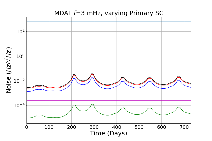
Using the the LISA orbit data, we also plot the modified dual arm locking noise curves for 2 years of the new LISA mission at $f=3~{\rm mHz}$ in Fig. 13. The top panel and the bottom left plot are plots corresponding to the 3 cases of SC1, SC2 and SC3 being the primary spacecraft respectively. At this frequency, we are dominated by the spacecraft motion at $10^{-2}{\rm Hz}/\sqrt{{\rm Hz}}$ for a significant part of the mission. This, similar to Fig. 12, corresponds to a noise suppression of $\mathcal{O}(10^{4})$ from the $30~{\rm Hz}/\sqrt{{\rm Hz}}$ pre-stabilized input laser frequency noise model. The only times at which the noise level goes above the TDI requirement are times at which $\Delta\tau\approx 0$ . Physically, these are times at which the differential arm has zero response, which forces a singularity in the integrator $(\frac{1}{s\Delta\tau})$ used to generate the arm response (Eq. 21)and hence causes large amplifications in clock noise, shot noise and spacecraft motion terms. We see that these times are different for the 3 different configurations. Hence, as shown in the bottom right plot of Fig. 13, allowing the switching of the primary spacecraft will enable us to maximize the value of $\Delta\tau$ and hence optimize the noise performance.

5 Conclusion

To summarize, following the footsteps of McKenzie et.al [17], we have estimated the modified dual arm locking noise performance for the new LISA mission. The new developments compared to [17] are the shorter arms, improved new clock noise levels and a new model for the spaceraft motion based on LISA Pathfinder data. In this work, we assume a cavity stabilized input laser noise and we tweak the controller design proposed by [17] to have more gain in the LISA band, by lowering the lower unity gain frequency. Doing so does worsen the Doppler frequency pulling rate but this new frequency pulling rate is still within the acceptable bounds of laser tuning range. In order to significantly improve the Doppler pulling characteristics at lock acquisition without sacrificing the gain in the LISA band, we also propose to increase the averaging time window for the initial Doppler estimate from $T=200\,{\rm seconds}$ to $T\approx 40000\,{\rm seconds}$ .

6 Acknowledgement

This work is supported by NASA grant 80NSSC20K0126.

References

[1] Pau Amaro-Seoane et al. Laser interferometer space antenna, 2017.
[2] J. Aasi et al. Advanced LIGO. Class. Quant. Grav., 32:074001, 2015.
[3] B. P. Abbott et al. LIGO: The Laser interferometer gravitational-wave observatory. Rept. Prog. Phys., 72:076901, 2009.
[4] T. Accadia et al. Virgo: a laser interferometer to detect gravitational waves. JINST, 7:P03012, 2012.
[5] F. Acernese et al. Advanced Virgo: a second-generation interferometric gravitational wave detector. Class. Quant. Grav., 32(2):024001, 2015.
[6] Yoichi Aso, Yuta Michimura, Kentaro Somiya, Masaki Ando, Osamu Miyakawa, Takanori Sekiguchi, Daisuke Tatsumi, and Hiroaki Yamamoto. Interferometer design of the KAGRA gravitational wave detector. Phys. Rev. D, 88:043007, Aug 2013.
[7] T. Akutsu et al. Overview of KAGRA: Detector design and construction history, 2020.
[8] H. Grote. The GEO 600 status. Class. Quant. Grav., 27:084003, 2010.
[9] K L Dooley et al. GEO 600 and the GEO-HF upgrade program: successes and challenges. Classical and Quantum Gravity, 33(7):075009, mar 2016.
[10] Stefanie Kroker and Ronny Nawrodt. The Einstein telescope. IEEE Instrum. Measur. Mag., 18(3):4–8, 2015.
[11] David Reitze, Rana X Adhikari, Stefan Ballmer, Barry Barish, Lisa Barsotti, GariLynn Billingsley, Duncan A. Brown, Yanbei Chen, Dennis Coyne, Robert Eisenstein, Matthew Evans, Peter Fritschel, Evan D. Hall, Albert Lazzarini, Geoffrey Lovelace, Jocelyn Read, B. S. Sathyaprakash, David Shoemaker, Joshua Smith, Calum Torrie, Salvatore Vitale, Rainer Weiss, Christopher Wipf, and Michael Zucker. Cosmic Explorer: The U.S. contribution to gravitational-wave astronomy beyond LIGO, 2019.
[12] Massimo Tinto and Sanjeev V Dhurandhar. Time-delay interferometry. Living Reviews in Relativity, 24(1):1, 2021.
[13] Massimo Tinto, F. B. Estabrook, and J. W. Armstrong. Time-delay interferometry for LISA. Phys. Rev. D, 65:082003, Apr 2002.
[14] LISA performance model and error budget, LISA-LCST-INST-TN-003. 2018.
[15] B Bachman, G de Vine, J Dickson, S Dubovitsky, J Liu, W Klipstein, K McKenzie, R Spero, A Sutton, B Ware, and C Woodruff. Flight phasemeter on the laser ranging interferometer on the GRACE follow-on mission. 840:012011, may 2017.
[16] B. S. Sheard, M. B. Gray, D. E. McClelland, and D. A. Shaddock. Laser frequency stabilization by locking to a LISA arm. Phys. Lett. A, 320:9–21, 2003.
[17] Kirk McKenzie, Robert E. Spero, and Daniel A. Shaddock. Performance of arm locking in lisa. Phys. Rev. D, 80:102003, Nov 2009.
[18] Yiu Yinan. Arm Locking for Laser Interferometer Space Antenna. PhD thesis, University of Florida, 2011.
[19] Andrew Sutton and Daniel A. Shaddock. Laser frequency stabilization by dual arm locking for LISA. Phys. Rev. D, 78:082001, Oct 2008.
[20] LISA frequency planning, LISA- AEI-INST-TN-002. 2018(unpublished).
[21] Massimo Tinto and Olaf Hartwig. Time-delay interferometry and clock-noise calibration. Phys. Rev. D, 98:042003, Aug 2018.
[22] M. Armano, H. Audley, J. Baird, P. Binetruy, M. Born, D. Bortoluzzi, E. Castelli, A. Cavalleri, A. Cesarini, A. M. Cruise, K. Danzmann, M. de Deus Silva, I. Diepholz, G. Dixon, R. Dolesi, L. Ferraioli, V. Ferroni, E. D. Fitzsimons, M. Freschi, L. Gesa, F. Gibert, D. Giardini, R. Giusteri, C. Grimani, J. Grzymisch, I. Harrison, G. Heinzel, M. Hewitson, D. Hollington, D. Hoyland, M. Hueller, H. Inchauspé, O. Jennrich, P. Jetzer, N. Karnesis, B. Kaune, N. Korsakova, C. J. Killow, J. A. Lobo, I. Lloro, L. Liu, J. P. López-Zaragoza, R. Maarschalkerweerd, D. Mance, N. Meshksar, V. Martín, L. Martin-Polo, J. Martino, F. Martin-Porqueras, I. Mateos, P. W. McNamara, J. Mendes, L. Mendes, M. Nofrarias, S. Paczkowski, M. Perreur-Lloyd, A. Petiteau, P. Pivato, E. Plagnol, J. Ramos-Castro, J. Reiche, D. I. Robertson, F. Rivas, G. Russano, J. Slutsky, C. F. Sopuerta, T. Sumner, D. Texier, J. I. Thorpe, D. Vetrugno, S. Vitale, G. Wanner, H. Ward, P. J. Wass, W. J. Weber, L. Wissel, A. Wittchen, and P. Zweifel. LISA pathfinder platform stability and drag-free performance. Phys. Rev. D, 99:082001, Apr 2019.