Hydrodynamic Relaxation in a Strongly Interacting Fermi Gas

Studies of thermodynamics and hydrodynamic transport in strongly correlated Fermi gases connect widely different forms of matter across vast energy scales Adams et al. 2012; Strinati et al. 2018; Bloch et al. 2012. Strongly interacting Fermi gases are created by tuning a trapped, two-component cloud near a collisional (Feshbach) resonance O’Hara et al. 2002. A resonantly interacting or unitary Fermi gas is of special interest, as it is a scale-invariant, strongly interacting quantum many-body system, with thermodynamic and transport properties that are universal functions of the density and temperature Ho 2004, permitting parameter-free comparisons with predictions.

However, the behavior of the shear viscosity $\eta$ and the thermal conductivity $\kappa_{T}$ of a unitary Fermi gas is not yet established. Measurement of hydrodynamic flow in freely expanding clouds Cao et al. 2011; Joseph et al. 2015 enables extraction of $\eta$ in the normal fluid regime, but requires a second order hydrodynamics model to properly account for ballistic flow in the dilute edges Bluhm and Schäfer 2016; Bluhm et al. 2017. Recent measurements of the sound diffusivity Patel et al. 2020, by sound attenuation in a driven, uniform density, unitary Fermi gas, constrain $\eta$ and $\kappa_{T}$, but they are not independently determined MZT.

In this Letter, we report new time-domain, free evolution methods for measuring hydrodynamic transport coefficients in a normal fluid unitary Fermi gas. We confine a cloud of ⁶Li atoms in a repulsive box potential, producing a sample of nearly uniform density. A density perturbation is then created, Fig. 1, by applying a small static optical potential that is spatially periodic along one axis. After equilibrium is established, the perturbing potential is abruptly extinguished. We measure the time-dependence of the dominant spatial Fourier component of the density, $\delta n(q,t)$, Fig. 2, which exhibits an exponentially decaying mode that measures the thermal conductivity and a decaying oscillatory mode that determines the sound speed and the sound diffusivity. The data are well fit by a linear hydrodynamics analytic model, enabling measurement of both the shear viscosity $\eta$ and the thermal conductivity $\kappa_{T}$.

The experiments employ ultracold ⁶Li atoms in a balanced mixture of the two lowest hyperfine states, which are evaporatively cooled in a CO₂ laser trap and loaded into a box potential. The box comprises six sheets of blue-detuned light, created by two digital micromirror devices (DMDs) Baird et al. 2019. The top and bottom sheets employ a 669 nm beam. The four vertically propagating sheets are produced by a 532 nm beam, which passes through a diffractive optical element and an imaging lens to produce a “top-hat” shaped intensity profile on the surface of the DMD array. The box potential $U_{0}(\mathbf{r})$ yields a rectangular density profile with typical dimensions $(x,y,z)=(52\times 50\times 150)\,\mu$m. The density varies slowly in the direction of the long ($z$) axis, due to the harmonic confining potential $\propto z^{2}$ arising from the curvature of the bias magnetic field, which has little effect on the shorter $x$ and $y$ axes. The typical total central density is $n_{0}=4.5\times 10^{11}$ atoms/cm³, with the Fermi energy $\epsilon_{\!F0}\equiv k_{B}T_{F}=k_{B}\times 0.22\,\mu$K and Fermi speed $v_{F}\simeq 2.5$ cm/s. The box depth $U_{0}\simeq 1.1\,\mu$K Sup.

Once the cloud is loaded into the box potential, we employ the 532 nm DMD to slowly ramp up an additional small optical potential $\delta U(z)$, which is spatially periodic along the $z$-axis. After thermal equilibrium is established, the cloud profile exhibits a periodic spatial modulation, $\delta n(z,0)$, Fig. 1. The measurements employ modulation amplitudes $\delta n/n_{0}$ from 7% to 19%, yielding consistent data within our error bars.

After the periodic potential is abruptly extinguished, we measure the oscillatory decay of the density change $\delta n(z,t)=n(z,t)-n_{0}(z)$. For each image, the signal $n$ and subtracted background $n_{0}(z)$ densities are scaled to their respective total atom number to suppress noise arising from shot to shot atom number variation. We perform a fast Fourier transform (FFT) of $\delta n(z,t)$ at each time, in a region containing an integer number (typically 3-4) of spatial periods near the peak density, minimizing the imaginary component to obtain a real transform, $\delta n(q,t)$, Fig. 2.

To model the data, where the initial conditions are isothermal, it is convenient to construct the coupled equations for the changes in the density $\delta n(z,t)$ and temperature $\delta T(z,t)$. We use the continuity equation to eliminate the velocity field. For experiments in the linear response regime Sup,

with $c_{T}$ the isothermal sound speed and $m$ the atom mass. Here, $\delta\tilde{T}=n_{0}\beta\,\delta T$ has dimension of density, with $\beta=-1/n(\partial n/\partial T)_{P}$ the thermal expansivity Sup and

with $\epsilon_{LP}\equiv c_{P_{1}}/c_{V_{1}}-1$ the Landau-Placzek parameter. The heat capacities per particle at constant volume $c_{V_{1}}$ and at constant pressure $c_{P_{1}}$ can be determined from the measured equation of state Ku et al. 2012; Sup.

Eqs. 1 and 2 have simple physical interpretations. The $c_{T}^{2}$ terms on the right-hand side of eq. 1 correspond to the pressure change Sup. A viscous damping force arises from the shear viscosity, $\eta\equiv\alpha_{\eta}\,\hbar n_{0}$, while the bulk viscosity $\xi_{B}$ vanishes for a unitary Fermi gas Bul. The final terms in eq. 1 arise from the perturbing and box potentials, where $\partial_{z}U_{0}(z)$ is found from the slowly varying background density $n_{0}(z)$ Sup and $\delta U(z,t>0)=0$ for our experiments. The first term on the right-hand side of eq. 2 describes the adiabatic change in the temperature due to the change in density. The last term describes temperature relaxation at constant density due to the heat flux, which is proportional to the thermal conductivity $\kappa_{T}\equiv\alpha_{\kappa}\,\hbar n_{0}\,k_{B}/m$. Eqs. 1 and 2 can be solved numerically for $\delta n(z,t)$, with the initial conditions $\delta n(z,0)$ (measured), $\delta\dot{n}(z,0)=0$, and $\delta\tilde{T}(z,0)=0$.

We find that a perturbation wavelength $\lambda\simeq 23\,\mu$m yields good dynamic range for decay measurements over time scales that avoid perturbing $\delta n(z,t)$ in the measured central region by reflections from the walls of box potential, which then can be neglected. Since $\delta U=0$, a spatial Fourier transform of eqs. 1 and 2 yields coupled equations for $\delta\ddot{n}(q,t)$ and $\delta\dot{\tilde{T}}(q,t)$. These determine the analytic fit function Sup,

where $A_{1}=A-A_{0}$ and $A_{2}=[(\Gamma-a)A_{0}+a\,A]/b$ satisfy two of the initial conditions $\delta n(q,0)=A$ and $\delta\dot{n}(q,0)=0$. The third initial condition $\delta\ddot{n}(q,0)=-c_{T}^{2}q^{2}A$ Sup determines $A_{0}=A(a^{2}+b^{2}-c_{T}^{2}\,q^{2})/[(\Gamma-a)^{2}+b^{2}]$.

We see that the solution consists of two independent modes, Fig. 2 (inset). One mode is exponentially decaying and determines the thermal diffusivity as discussed below. The other is a decaying, oscillating first sound mode, which determines the sound diffusivity. Together, the decay rates of these two distinct modes determine both the thermal conductivity and the shear viscosity.

The frequencies $\Gamma$, $a$, and $b$ in eq. 3 are related to the frequencies $\gamma_{\eta}\equiv 4\eta\,q^{2}/(3n_{0}m)$, $\gamma_{\kappa}\equiv\kappa_{T}q^{2}/(n_{0}c_{V_{1}})$, and $c_{T}q$ by Sup

Here, $c_{S}$ and $c_{T}$ are the adiabatic and isothermal sound speeds, which obey $c_{S}^{2}/c_{T}^{2}=c_{P_{1}}/c_{V_{1}}=1+\epsilon_{LP}(T/T_{F})$.

Fitting eq. 3 to the data yields the red curve in Fig. 2, with the three frequencies $c_{T}q,\gamma_{\eta},\gamma_{\kappa}$, and the amplitude $A$ as free parameters. We find that fitting the data with $A_{0}=0$ increases the $\chi^{2}$ per degree of freedom from $\simeq 1$ to $\simeq 20$, demonstrating the importance of the thermal diffusion mode, which determines the thermal conductivity in our measurements.

The reduced temperature $T/T_{F}=\theta(c_{T}/v_{F})$ in eqs. 4-6 is self-consistently determined from $c_{T}$ by the equation of state Ku et al. 2012; Sup, with $v_{F}$ given for the average central density $n_{0}$ Sup. The fits determine the frequency $c_{T}q$ within 2%, enabling in-situ thermometry The.

We note that in the long wavelength (LW) limit, where $c_{S}\,q>>\gamma_{\kappa},\gamma_{\eta}$, eq. 5 requires $b/q\simeq c_{S}$, the first sound speed. Then eq. 6 reduces to $\Gamma/q^{2}\simeq\kappa_{T}/(n_{0}c_{P_{1}})=D_{T}$, the thermal diffusivity, and eq. 4 yields $2\,a/q^{2}\simeq\gamma_{\eta}/q^{2}+\gamma_{\kappa}/q^{2}-\Gamma/q^{2}=D_{1}$, the usual first sound diffusivity Sup; Landau and Lifshitz 1959. In our experiments, where $\lambda\simeq 23\,\mu$m, we find that $b/q$ is smaller than $c_{S}$ by 2.2 %, 4.3 % and 5.7 % for $T/T_{F}=0.28,0.46,$ and $0.63$, respectively, close to the LW limit.

Further, the LW limit requires $A_{0}/A=1-c_{V_{1}}/c_{P_{1}}$, which is $\simeq 0.3$ for our $T/T_{F}$ range and within $10\,$% of the measured values. As a cross check, we fit the data with eq. 3, letting both $A$ and $A_{0}$ be free parameters, and obtain consistent results for $A_{0}/A$.

We also estimate the change in the energy per particle $W_{1}$ that arises from the energy stored in the initial spatially periodic density profile. Assuming adiabatic compression, we find Sup,

For $\delta n/n_{0}\simeq 0.2\cos(qz)$, we have $W_{1}\simeq 0.01\,mc_{S}^{2}$. As $mc_{S}^{2}=10/9\,E_{1}$, with $E_{1}$ the energy per particle Patel et al. 2020; Sup, the change in $E_{1}$, and hence in $\theta=T/T_{F}$, is negligible.

Our measured shear viscosity, Fig. 3, can be compared to the high temperature diluteness expansion of Bluhm et al., Bluhm et al. 2017, $\eta_{\rm exp}(\theta)=(\alpha_{0}\,\theta^{3/2}+\alpha_{2})\,\hbar n$, where $\alpha_{0}=2.77(21)$ and $\alpha_{2}=0.25(08)$ are measured by using a second order hydrodynamics model to fit aspect ratio data for freely expanding clouds Joseph et al. 2015. Here, the first term is the high temperature limit, where $\theta^{3/2}n\propto T^{3/2}$ depends only on the temperature. The extracted $\alpha_{0}$ is in excellent agreement with a variational calculation based on the two-body Boltzmann equation for a unitary gas Bruun and Smith 2007; Bluhm et al. 2017. The leading correction from $\alpha_{2}$ depends only on the density. The red curve in Fig. 3 shows that $\eta_{\rm exp}(T/T_{F})$ is in agreement with the measurements in the box potential for $T/T_{F}\geq 0.45$. For comparison, the red-dashed curve shows the high temperature limit, where $\alpha_{2}=0$. The top purple-dashed curve is the T-matrix theory prediction of Enss et al., Enss et al. 2011, in reasonable agreement with the data.

In all of the figures, we compare data for $\lambda\simeq 23\,\mu$m to data points with $\lambda=18.2\,\mu$m, $18.9\,\mu$m, $32.3\,\mu$m (3-spatial periods) and $41.7\,\mu$m (2-spatial periods). These measurements show that there are no large systematic shifts with wavelength.

Our measured thermal conductivity, Fig. 4, can be compared with variational calculations for a unitary Fermi gas in the high temperature, two-body Boltzmann equation limit Braby et al. 2010, where $\kappa_{T}(\theta)=15/4\,\alpha_{0}\,\theta^{3/2}\,\hbar n\,k_{B}/m$, with $k_{B}$ the Boltzmann constant. The red-dashed line in Fig. 4 shows that the high temperature prediction is in reasonable agreement with measurements in the box potential for $T/T_{F}\geq 0.45$, without a temperature-independent correction, but the data are significantly smaller than predicted Frank et al. 2020; Zhou and Ma 2021.

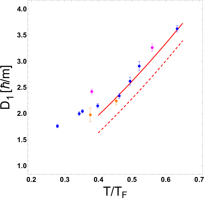
The sound diffusivity $D_{1}=2\,a/q^{2}$, in units of $\hbar/m$, Fig. 5, is determined by eqs. 4-6 from the fit parameters $c_{T}q$, $\gamma_{\eta}$, and $\gamma_{\kappa}$. We obtain the same results within our error bars, by directly fitting $\Gamma$, $a$ and $b$ in eq. 3, constraining $A_{0}/A$ using the long wavelength (LW) limit, where $b\simeq c_{S}q$ determines $T/T_{F}$. The red-dashed curve shows the predicted LW $D_{1}$, using the high temperature limits for both the shear viscosity and the thermal conductivity, with $c_{P_{1}}=5/2\,k_{B}$ and $c_{V_{1}}=3/2\,k_{B}$. For the red solid curve, the high temperature shear viscosity term in $D_{1}$ is replaced with the measured viscosity for the expanding gas, $\eta_{exp}(\theta)$, yielding a good fit for the higher temperature measurements, consistent with our measured $\eta$ and $\kappa_{T}$. Our diffusivity data can be compared to that of Patel et al., Patel et al. 2020, which is shifted upward relative to that of Fig. 5, but exhibits nearly identical scaling with $T/T_{F}$, as discussed in the supplementary material Sup.

In conclusion, we have independently determined the shear viscosity and thermal conductivity of a normal-fluid unitary Fermi gas in a box potential, directly from the two-mode oscillatory decay of a spatially periodic density perturbation. For the isothermal static initial conditions employed in the experiments, the thermally diffusive mode comprises $\simeq 30$% of the initial total amplitude of the dominant Fourier component, which is readily apparent in the free hydrodynamic relaxation. This method is complementary to frequency domain techniques, where transport properties of quantum fluids have been determined by measuring the hydrodynamic linear susceptibility Hohenberg and Martin 1965; Hu et al. 2018; Zhang and Yu 2018. For reduced temperatures $T/T_{F}>0.45$, we find that the shear viscosity measured by free hydrodynamic relaxation in a box potential is consistent with that extracted from data on expanding clouds Bluhm and Schäfer 2016; Bluhm et al. 2017, which includes a significant density-dependent contribution. At lower temperatures, $T/T_{F}<0.4$, the shear viscosity measured in the box is consistently larger than that of the expanding cloud. The thermal conductivity for $T/T_{F}>0.45$ is close to the high temperature limit. In contrast to the shear viscosity, the pure density dependent contribution to the high temperature thermal conductivity appears to be quite small. These results emphasize the need for rigorous calculations of the leading density-dependent corrections to the two-body high temperature limits. Finally, we expect that in the superfluid regime, the exponentially decaying mode will evolve into an oscillating second sound mode, which we hope to study in future experiments.

We thank Thomas Schäfer for stimulating discussions and Parth Patel and Martin Zwierlein for providing their sound diffusivity data in table form. Primary support for this research is provided by the Physics Divisions of the National Science Foundation (PHY-2006234) and the Air Force Office of Scientific Research (FA9550-16-1-0378).

^∗Corresponding author: jethoma7@ncsu.edu

References

- Adams et al. (2012) A. Adams, L. D. Carr, T. Schäfer, P. Steinberg, and J. E. Thomas, “Strongly correlated quantum fluids: ultracold quantum gases, quantum chromodynamic plasmas and holographic duality,” New J. Phys. 14, 115009 (2012).
- Strinati et al. (2018) G. C. Strinati, P. Pieri, Gerd Röpke, P. Schuck, and M. Urban, “The BCS-BEC crossover: From ultra-cold Fermi gases to nuclear systems,” Physics Reports 738, 1–76 (2018).
- Bloch et al. (2012) I. Bloch, J. Dalibard, and S. Nascimbène, “Quantum simulations with ultracold quantum gases,” Nature Physics 8, 267 (2012).
- O’Hara et al. (2002) K. M. O’Hara, S. L. Hemmer, M. E. Gehm, S. R. Granade, and J. E. Thomas, “Observation of a strongly interacting degenerate Fermi gas of atoms,” Science 298, 2179 (2002).
- Ho (2004) T.-L. Ho, “Universal thermodynamics of degenerate quantum gases in the unitarity limit,” Phys. Rev. Lett. 92, 090402 (2004).
- Cao et al. (2011) C. Cao, E. Elliott, J. Joseph, H. Wu, J. Petricka, T. Schäfer, and J. E. Thomas, “Universal quantum viscosity in a unitary Fermi gas,” Science 331, 58 (2011).
- Joseph et al. (2015) J. A. Joseph, E. Elliott, and J. E. Thomas, “Shear viscosity of a unitary Fermi gas near the superfluid phase transition,” Phys. Rev. Lett. 115, 020401 (2015).
- Bluhm and Schäfer (2016) M. Bluhm and T. Schäfer, “Model-independent determination of the shear viscosity of a trapped unitary Fermi gas: Application to high-temperature data,” Phys. Rev. Lett. 116, 115301 (2016).
- Bluhm et al. (2017) Marcus Bluhm, Jiaxun Hou, and Thomas Schäfer, “Determination of the density and temperature dependence of the shear viscosity of a unitary Fermi gas based on hydrodynamic flow,” Phys. Rev. Lett. 119, 065302 (2017).
- Patel et al. (2020) Parth B. Patel, Zhenjie Yan, Biswaroop Mukherjee, Richard J. Fletcher, Julian Struck, and Martin W. Zwierlein, “Universal sound diffusion in a strongly interacting Fermi gas,” Science 370, 1222–1226 (2020).
- (11) A new method for directly measuring temperature waves has been reported recently, accessing second sound and thermal diffusion in a unitary Fermi gas. See Z. Yan, P. B. Patel, B. Mukherjee, R. Fletcher, and M. W. Zwierlein, DAMOP21/Session/U07.2.
- Baird et al. (2019) Lorin Baird, Xin Wang, Stetson Roof, and J. E. Thomas, “Measuring the hydrodynamic linear response of a unitary Fermi gas,” Phys. Rev. Lett. 123, 160402 (2019).
- (13) See the Supplemental Material for discussions of the linearized hydrodynamic equations, the analytic solution, the forces arising from the box potential, the determination of the density, and the systematic error arising from the density variation.
- Ku et al. (2012) M.J. Ku, A. T. Sommer, L. W. Cheuk, and M. W. Zwierlein, “Revealing the superfluid lambda transition in the universal thermodynamics of a unitary Fermi gas,” Science 335, 563 (2012).
- (15) For a unitary Fermi gas, the bulk viscosity has been measured Elliott et al. 2014 and found to be negligible compared to the shear viscosity, consistent with predictions that for scale invariant systems Son 2007; Hou et al. 2013.
- (16) We give for the average central density Sup.
- Landau and Lifshitz (1959) L. D. Landau and E. M. Lifshitz, Fluid Dynamics, Course of Theoretical Physics Vol. VI (Pergamon Press, Oxford, 1959).
- Enss et al. (2011) T. Enss, R. Haussmann, and W. Zwerger, “Viscosity and scale invariance in the unitary Fermi gas,” Annals Phys. 326, 770–796 (2011).
- (19) The vertical error bars in Figs. 3 and 4 denote , where is the error matrix obtained from with and fixed. For the diffusivity in Fig. 5, is found by minimizing with respect to and , holding fixed in eq. 3. We estimate a systematic downward shift of %, arising from the density variation Sup.
- Bruun and Smith (2007) G. M. Bruun and H. Smith, “Shear viscosity and damping for a Fermi gas in the unitary limit,” Phys. Rev. A 75, 043612 (2007).
- Braby et al. (2010) Matt Braby, Jingyi Chao, and Thomas Schäfer, “Thermal conductivity and sound attenuation in dilute atomic Fermi gases,” Phys. Rev. A 82, 033619 (2010).
- Frank et al. (2020) Bernhard Frank, Wilhelm Zwerger, and Tilman Enss, “Quantum critical thermal transport in the unitary Fermi gas,” Phys. Rev. Research 2, 023301 (2020).
- Zhou and Ma (2021) Hang Zhou and Yongli Ma, “Thermal conductivity of an ultracold Fermi gas in the BCS-BEC crossover,” Sci. Rep. 11, 1228 (2021).
- Hohenberg and Martin (1965) P.C. Hohenberg and P.C. Martin, “Microscopic theory of superfluid helium,” Annals Phys. 34, 291–359 (1965).
- Hu et al. (2018) Hui Hu, Peng Zou, and Xia-Ji Liu, “Low-momentum dynamic structure factor of a strongly interacting Fermi gas at finite temperature: A two-fluid hydrodynamic description,” Phys. Rev. A 97, 023615 (2018).
- Zhang and Yu (2018) Pengfei Zhang and Zhenhua Yu, “Energy-absorption spectroscopy of unitary Fermi gases in a uniform potential,” Phys. Rev. A 97, 041601 (2018).
- Li et al. (2022) Xi Li, Xiang Luo, Shuai Wang, Ke Xie, Xiang-Pei Liu, Hui Hu, Yu-Ao Chen, Xing-Can Yao, and Jian-Wei Pan, “Second sound attenuation near quantum criticality,” Science 375, 528–533 (2022).
- Elliott et al. (2014) E. Elliott, J. A. Joseph, and J. E. Thomas, “Observation of conformal symmetry breaking and scale invariance in expanding Fermi gases,” Phys. Rev. Lett. 112, 040405 (2014).
- Son (2007) D. T. Son, “Vanishing bulk viscosities and conformal invariance of the unitary Fermi gas,” Phys. Rev. Lett. 98, 020604 (2007).
- Hou et al. (2013) Yan-Hua Hou, Lev P. Pitaevskii, and Sandro Stringari, “Scaling solutions of the two-fluid hydrodynamic equations in a harmonically trapped gas at unitarity,” Phys. Rev. A 87, 033620 (2013).
Appendix A Supplemental Material
In this supplemental material, we derive a linear hydrodynamics model to analyze the free oscillatory decay of a spatially periodic density perturbation in a normal fluid unitary Fermi gas. An analytic fit function is found for the time-dependence of the dominant spatial Fourier component, which determines the sound speed, the shear viscosity, and the thermal conductivity. We discuss the sound diffusivity, the thermodynamics employed in the model, the energy stored in the initial periodic density profile, the determination of the 3D density, and the systematic error arising from the density variation.
A.1 Hydrodynamic linear response for a normal fluid.
We consider a normal fluid Fermi gas, which is a single component fluid with a mass density is , where is the total particle density (we assume a 50-50 mixture of two components) and is the atom mass. satisfies the continuity equation,