∎
On the Complexity of the Geometric Median Problem with Outliers
Abstract
In the Geometric Median problem with outliers, we are given a finite set of points in -dimensional real space and an integer , the goal is to locate a new point in space (center) and choose of the input points to minimize the sum of the Euclidean distances from the center to the chosen points. This problem can be solved “almost exactly” in polynomial time if is fixed and admits an approximation scheme PTAS in high dimensions. However, the complexity of the problem was an open question. We prove that, if the dimension of space is not fixed, Geometric Median with outliers is strongly NP-hard, does not admit approximation schemes FPTAS unless PNP, and is W[]-hard with respect to the parameter . The proof is done by a reduction from the Independent Set problem. Based on a similar reduction, we also get the NP-hardness of closely related geometric -clustering problems in which it is required to partition a given set of points into two balanced clusters minimizing the cost of median clustering. Finally, we study Geometric Median with outliers in space and prove the same complexity results as for the Euclidean problem.
Keywords:
Geometric median Outlier detection Capacitated -Median Single location problem Balanced clustering ComplexityMSC
68Q25 90C27 90B85 62071 Introduction
We give an answer to the open question on the complexity of the Geometric Median problem with outliers, which is an extension of the classical problem of finding the geometric median (“minisum point”) of given points in Euclidean space.
Let denote values of the Euclidean norm. The problem we consider is formulated as follows:
Geometric Median with outliers. Given an -element set in space and an integer . Find a center and an -element subset to minimize the value of
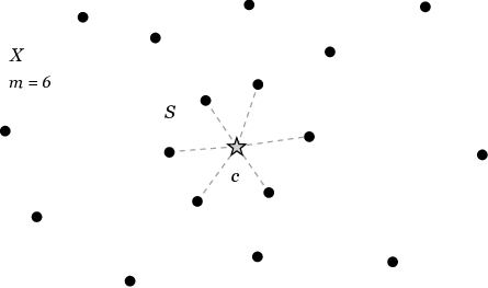
This problem may also be referred to as Capacitated Euclidean -Median. In fact, we need to find a center minimizing the total distance from to nearest input points (see Fig. 1). In an equivalent version, we need to find a center maximizing the cardinality of a subset for which the value of does not exceed a given upper bound.
As in the usual Geometric Median problem, where , the input points are considered as clients or demand points, while the desired center, as a location for placing a facility to serve the clients. The clients which are removed from this service in the solution are called outliers. The problem with outliers arises naturally in the following situations:
-
The facility to be placed at the center we are looking for has a limited capacity and may not serve all the demand points.
-
There exist an upper limit for the transportation cost, so we need to remove a minimum possible number of clients from the service to satisfy this limit.
-
The data contains noise and errors. In this case, a few most distant clients may exert a disproportionately strong influence over the final solution and correspond to the least robust input points.
-
The discovered outliers do not fit the rest of the data and are worthy of further investigation. In particular, once identified, they can be used to discover anomalies in the data.
Besides the practical considerations mentioned above, the problem is theoretically interesting. Strictly speaking, no polynomial-time algorithms are known even for the problem without outliers, where we find the geometric median of the whole set . However, one can say that the usual Geometric Median problem is polynomially solvable “almost exactly” since, e.g., the algorithm from Cohen computes its -approximate solution in time .
The problem with outliers seems to be cardinally harder due to the exponential number of the subsets . The first idea how to solve it is using the property that optimal subsets consist of input points nearest to some point in space. It allows to find an optimal solution by enumerating the cells of the -order Voronoi diagram for the set and calculating the geometric medians of the subsets corresponding to these cells. So, by using the known algorithms for constructing high-order Voronoi diagrams ERS; ESS and for finding geometric medians Cohen, we compute a -approximate solution of the Geometric Median problem with outliers in time . Thus, in the case of fixed , we can solve the problem “almost exactly” in polynomial time.
If the dimension of space is not fixed, a more effective idea is to use the approximation algorithm from Shen2019; Shen2020 for the following general clustering problem, which contains Geometric Median with outliers:
General Problem. Given points in space , integers , unit distance costs , and powers , , , where is some constant. Find disjoint subsets of total cardinality and select a tuple to minimize the value of
The framework suggested in Shen2019; Shen2020; Shen2021d allows to find a -approximate solution of General Problem in time for any fixed . This framework is based on constructing a polynomial-cardinality set of points which approximate all the points of space with respect to the distances to the input points. Thus, in our case, we have an approximation scheme PTAS with running time .
Related problems. ElGindy and Keil ElGindy consider the equivalent version of the Geometric Median problem with outliers where it is required to find a maximum-cardinality subset of input points satisfying a given upper bound for the cost of the geometric median. They suggest an -time exact algorithm for the two-dimensional case with or distances.
Two well-known single location problems closest to Geometric Median with outliers are Smallest -Enclosing Ball and -Variance. The first consists of finding input points minimizing the radius of the ball enclosing these points. In the second, we need to find input points minimizing the sum of the squared distances from these points to their mean. In high dimensions, both problems are strongly NP-hard Shen2013; Shen2015; KP but admit approximation schemes with running time AHV2005 and Shen2012 respectively.
Finally, note that the discrete version of -Median with outliers, in which all the centers must be selected from a given finite set, and also -Means with outliers, Uncapacitated Facility Location with outliers, and other similar problems were considered by Charikar et al. Charikar, Chen Chen2008, Cohen-Addad et al. CFS, and Krishnaswamy et al. KLS. In particular, they suggest constant-factor algorithms for these problems in the case of non-fixed .
Our contributions. Surprisingly, the complexity of Geometric Median with outliers was an open question. We prove that, in high dimensions, this problem is strongly NP-hard, does not admit approximation schemes FPTAS unless PNP, and is W[]-hard with respect to the parameter . The proof is based on a reduction from the Independent Set problem. The main idea of this reduction is constructing instances in which the geometric median of any subset of points corresponding to vertices of a given graph is well approximated by the mean of these points, while the total distance from the points to their mean monotonously depends on the number of edges between the corresponding vertices.
By using a similar reduction from the problem of finding a maximum bisection in a -regular graph, we get the NP-hardness and the non-existence of approximation schemes FPTAS for the following closely related problems:
Equal-Size Geometric -Median. Given an -element set in space , where is even. Find centers and a partition of into two equal-size subsets and to minimize the value of .
Balanced Geometric -Median. Given an -element set in space . Find centers and a partition of into two subsets and to minimize the value of .
Additionally, we study the -Median problem with outliers, which consists of finding a center minimizing the sum of the distances to input points. For this problem, the same complexity results are proved as for the Euclidean case.
2 Complexity of the Euclidean problem
In this section, we prove the hardness of finding an optimum -element subset in the case when the distances between input points and the desired center are defined by the Euclidean norm.
2.1 Reduction from Independent Set
We construct a reduction to Geometric Median with outliers from the classic NP-hard problem of determining the existence of an independent set of a given cardinality in a general graph.
Let be any undirected graph on some -element set of vertices . First, construct the following auxiliary graph . The vertices of are the same as in and the set of edges contains all the edges of and also copies of the loop edge for each vertex , where is the degree of in . So each vertex in is incident to exactly edges (see Fig. 2). Then fix an arbitrary orientation on the edges of : for every non-loop edge, choose an endpoint of this edge which it is “outgoing from” and one which it is “incoming to”. For definiteness, we will assume that every loop edge is “incoming to” its endpoint. Denote by the set of edges of . Next, map each vertex to the point with the following coordinates: , where is some big integer which will be specified later; for every edge outgoing from and for ones incoming to ; all the other coordinates are zero (see Fig. 2). Finally, define the instance of the Geometric Median problem with outliers corresponding to the graph as the set .

Comment 1.
Adding the loop edges and selecting an edge orientation in the auxiliary graph provide that all the vectors , , have the same number of the coordinates and, for any two vectors , the sets of their non-zero coordinates are either disjoint or intersecting by the only coordinate , for which . As a corollary, the distance between the vectors and for any adjacent different vertices is greater than that for non-adjacent ones. Indeed, , where denotes the projection of into space , while the value of is if the vertices and are adjacent and is otherwise.
Comment 2.
Setting the coordinates , , equal to a big value of provides that the geometric median of any subset is close to its mean, while, as it will be proved, the total distance from the points to their mean has an almost affine dependence on the sum of pairwise squared distances between the corresponding vectors .
Idea of the reduction. We will prove that, given an -element subset of vertices , the minimum value of , where , over all monotonously depends on the number of the edges in the original graph connecting the vertices of to each other. Therefore, if the set is an optimal solution of Geometric Median with outliers for the given , then is an -element subset of vertices with the minimum number .
For any finite set , denote by and the mean and the geometric median of this set respectively:
Let be any subset of vertices with an arbitrary cardinality . Put , , , and for each . Then is the zero vector and the following property holds:
Property 1.
;
, where .
Proof.
(a) Given a vector , let . Then it is easy to see that the set consists of the loops in and the edges connecting and . Hence, we have . Next, the set consists of all the elements of and also the edges connecting and the other vertices of . So , where is the degree of in the subgraph of induced by . For coordinates , the values of are ; for coordinates, these values are ; for the other coordinates from , these values are . Then
But and , so . The latter is maximized when , therefore, we have .
On the other hand, we have , , and , so
But it can be easily proved that for all . It follows that .
(b) Obviously, we have , which implies the required equation.
The main geometric statement underlying the proposed reduction is that the distance between and is very close to zero for big : if . This statement will be proved in Section 2.2 (Lemma 5).
Lemma 1
Suppose that . Then, for some , we have
Proof.
By the cosine theorem, we have
where is the dot product. Property 1, Lemma 5, and the condition for yield that
so . On the other hand, Taylor’s theorem (in the Lagrange remainder form) implies the equation
Therefore,
where . Since is the zero vector, the sum of the terms is zero. Then, taking into account the inequality and the above observations, we obtain that
where and .
Next, calculate the value of . Given a vertex , consider the projection of the vector into space . It is easy to see that the value of equals the squared distance from the vector to the mean of these vectors. But it is well-known (e.g., see Inaba; Shen2012) that the sum of such squared distances equals the sum of all the pairwise squared distances divided by :
At the same time, by the construction of the vectors , each pairwise squared distance equals if the vertices and are adjacent and equals otherwise (see Comment 1). So we have
It follows the required equation. The lemma is proved.
Theorem 2.1
Geometric Median with outliers is strongly NP-hard, does not admit approximation schemes FPTAS unless PNP, and is W-hard with respect to the parameter .
Proof.
Suppose that is any -vertex graph, is any -element subset of its vertices, where , and put . Then and, by Lemma 1, we have the equation , where
and . By the choice of , the absolute value of the latest term in this expression is at most times of . Therefore, is an independent set in the graph if and only if . Thus, the Independent Set problem is reduced to Geometric Median with outliers. Taking into account that is an integer bounded by a polynomial in the length of the input, it gives the strong NP-hardness of the latter problem.
Moreover, by the above, if , then
On the other hand, both values and are less than , which implies that Geometric Median with outliers is NP-hard to approximate within a factor of . But, for an arbitrary polynomial , any approximation scheme FPTAS allows to get a -approximation in polynomial time. Therefore, the existence of such schemes is impossible unless PNP.
Finally, note that the constructed reduction can be represented as a parameterized reduction of the W[]-hard Independent Set problem parameterized by Downey to Geometric Median with outliers parameterized by . It follows the statement on the W[]-hardness. The theorem is proved.
Balanced Geometric -Median clustering
Based on the same construction of the set , we can give similar reductions from the well-known NP-hard problem of finding a maximum bisection in a -regular graph Feige to the Equal-Size and Balanced Geometric -Median problems.
Indeed, in a -regular graph, the number of the edges connecting an -element subset of vertices with its complement equals . Therefore, by Lemma 1, the minimum value of in the case when corresponds to a bisection with the maximum number of crossing edges. It gives the NP-hardness and the non-existence of approximation schemes FPTAS for Equal-Size Geometric -Median.
To get the similar result for Balanced Geometric -Median, we need to note that the value of the objective function of this problem on the bipartition , equals the expression
where and . But this expression can be approximated by the value of for big . It follows that the minimum of is attained when and, by the above observations, corresponds to a maximum bisection.
2.2 Location of the geometric median
In this section, we prove the upper bound for the distance between the geometric median and the mean of the set underlying Lemma 1.
Let be an arbitrary -element subset of . Since the mean of any single- and two-element set is also its geometric median, we will assume that .
Rough estimations
First, we prove some rough estimation for the value which will be needed for the proof of the stronger upper bound.
We start by introducing some notations. Given a set , denote by the affine hull of this set. Denote by the subspace in space consisting of all the vectors with the zero edge coordinates: , . Given a vertex of the graph , define the point for which and all the other coordinates are zero. In other words, the vector is the orthogonal projection of into the space . Note that the distance from the mean of the set to each of its elements is .
Lemma 2
The geometric median of the set coincides with its mean. Moreover, if a vector is orthogonal to the affine space , then the minimum of the value subject to is attained at .
Proof.
The derivative of the function along any coordinate is
So the value of this derivative at the point is
It follows that the point is the geometric median of the set .
Then the derivative of the function along any direction in the affine space is equal to zero at the point : . On the other hand, the derivative of the function along any direction in is
So the value of this derivative at the point is
It follows that the point is the minimum of the function subject to . The lemma is proved.
Lemma 3
Suppose that and , . Then, for each , the following holds: .
Proof.
Let be the orthogonal projection of the point into the space . Then and since the set is the projection of the set into . Next, consider the affine subspace in orthogonal to the vector and passing through the point . Denote by the intersection point of this subspace with the line passing through the points and (see Fig. 3). Then is the point nearest to in . On the other hand, it is easy to see that can be obtained by shifting the affine subspace by the vector and is orthogonal to . Hence, applying Lemma 2 to the set , we get that the point is the minimum of the function subject to . It follows that .

By the cosine theorem, we have
where . At the same time,
Then, since , we get the inequality
which implies that
Taking into account that and, therefore, , we have
So if .
It remains to note that the vectors and are orthogonal to the space and, therefore, to the vector . But the vector is also orthogonal to by the choice of . Thus, we obtain that
which equals in absolute value. The lemma is proved.
Lemma 4
Suppose that . Then .
Proof.
For every , consider the plane containing the points , , and the origin 0. Note that this plane is orthogonal to the affine space since the line is orthogonal to and is contained in . At the same time, the projection of the point into the space lies in . So the orthogonal projection of the point into the plane belongs to the intersection of with , i.e., lies on the line (see Fig. 4).

Then
where is the angle between the lines and . Taking into account the equation and Lemma 3, it follows that the absolute value of the -th coordinate of the vector is less than . On the other hand, for each edge incident to , the absolute value of the -th coordinate of this vector is at most since the geometric median is a convex combination of the points , . For every other coordinate and every , we have , which implies that . Thus, we obtain the inequality , so . The lemma is proved.
A tighter estimation
Now, we get the tighter estimation for the geometric median location which is used in Section 2.1. We start by proving the following geometric properties of the vectors , .
Property 2.
If , then the angle between the vectors and for different lies in the interval .
Proof.
Indeed, . The first term in this expression is ; the second is at least and is at most . Then, taking into account Property 1(a), we obtain that the cosine of the angle between the vectors and is between the values and . It remains to note that and that is sufficiently big, so we have and .
Property 3.
If , then .
Proof.
By Property 2, the angles between the vectors and for are at least . So there exists at most one vector , , such that the angles between and are at most some . Then , where . Note that and that this expression has the only local extremum on , at the point . Therefore, we have , which equals if .
Property 4.
If , then .
Proof.
By Property 1(a), we have , where is bounded by the value . Since is the zero vector, it follows the inequality . Next, by using the observations from the proof of Property 3, we obtain that , where
Therefore, the multiplier equals , which is less than .
Lemma 5
Suppose that . Then .
Proof.
We will compare the values of and . The first is
while the second is
Note that and
by Property 1, Lemma 4, and the condition for . On the other hand, Taylor’s theorem (in the Lagrange remainder form) implies the equation
Therefore, and
Since is the zero vector, the sums of the terms are zero. On the other hand, by Properties 4 and 1, the sum of the terms is greater than . At the same time, by Properties 3 and 1, the sum of the terms is greater than . Therefore, the inequality implies that
Recall that by Lemma 4. Then, taking into account the obvious inequality for and , we have
But , so
Since is sufficiently big, it follows that . The lemma is proved.
3 The case of distances
To prove the statements of Theorem 2.1 for the case of distances, we construct a similar but much simpler reduction from the Independent Set problem.
Let be any -vertex undirected graph. Without loss of generality, we will assume that has no isolated vertices. Fix an arbitrary orientation on its edges: for every edge, choose an endpoint of this edge which it is “outgoing from” and one which it is “incoming to”. Next, map each vertex to the point with the following coordinates: for every edge outgoing from and for ones incoming to ; all the other coordinates are zero (see Fig. 5). Note that, since has no isolated vertices, all the vectors , , are distinct. Define the instance of the -Median problem with outliers corresponding to the graph as the set .

Comment 3.
Selecting an edge orientation provides that the -distance between the vectors for adjacent different vertices is , while that for non-adjacent ones is . It will be used below to justify the proposed reduction.
Estimate the value of the -median cost of the set for an arbitrary -element subset of vertices , where . Consider the point for which (or ) if the edge is outgoing from and incoming to (or vice versa), otherwise, . Note that, if the set is independent, then any edge which is incident to vertices from is either outgoing from or incoming to . In this case, the -distance from to each point , , is exactly , so .
On the other hand, for any subset and any point , we have
Moreover, by Comment 3, if the set contains at least two adjacent vertices and , then
It follows that the -median cost of the set is if the set is independent and is at least otherwise. Thus, the Independent Set problem is reduced to -Median with outliers and we obtain the following theorem:
Theorem 3.1
The -Median problem with outliers is strongly NP-hard, does not admit approximation schemes FPTAS unless PNP, and is W-hard with respect to the parameter .
References
- (1) Agarwal P.K., Har-Peled S., Varadarajan K.R. Geometric approximation via coresets // Combinatorial and Computational Geometry, MSRI Publications 52, 1–30 (2005) http://library.msri.org/books/Book52/files/01agar.pdf
- (2) Charikar M., Khuller S., Mount D.M., Narasimhan G. Algorithms for facility location problems with outliers // Proc. 12th ACM-SIAM Symposium on Discrete Algorithms (SODA 2001), 642–651 (2001) https://dl.acm.org/doi/10.5555/365411.365555
- (3) Chen K. A constant factor approximation algorithm for -median clustering with outliers // Proc. 19th ACM-SIAM Symposium on Discrete Algorithms (SODA 2008), 826–835 (2008) https://dl.acm.org/doi/10.5555/1347082.1347173
- (4) Cohen M.B., Lee Y.T., Miller G., Pachocki J., Sidford A. Geometric median in nearly linear time // arXiv:1606.05225 [cs.DS] (2016) https://arxiv.org/abs/1606.05225
- (5) Cohen-Addad V., Feldmann A.E., Saulpic D. Near-linear time approximations schemes for clustering in doubling metrics // Proc. 60th Symposium on Foundations of Computer Science (FOCS 2019), 540–559 (2019) https://doi.org/10.1109/FOCS.2019.00041
- (6) Downey R.G., Fellows M.R. Fundamentals of Parameterized Complexity. Texts in Computer Science. Springer-Verlag, London (2013) https://doi.org/10.1007/978-1-4471-5559-1
- (7) Edelsbrunner H., O’Rourke J., Seidel R. Constructing arrangements of lines and hyperplanes with applications // SIAM J. Computing 15(2), 341–363 (1986) https://doi.org/10.1137/0215024
- (8) Edelsbrunner H., Seidel R., Sharir M. On the zone theorem for hyperplane arrangements // SIAM J. Computing 22(2), 418–429 (1993) https://doi.org/10.1137/0222031
- (9) ElGindy H., Keil J.M. Efficient algorithms for the capacitated -median problem // ORSA J. Computing 4(4), 418–425 (1992) https://doi.org/10.1287/ijoc.4.4.418
- (10) Feige U., Karpinski M., Langberg M. A note on approximating max-bisection on regular graphs // Inf. Proc. Letters 79(4), 181–188 (2001) https://doi.org/10.1016/S0020-0190(00)00189-7
- (11) Inaba M., Katoh N., Imai H. Applications of weighted Voronoi diagrams and randomization to variance-based -clustering // Proc. 10th ACM Symposium on Computational Geometry, 332–339 (1994) https://doi.org/10.1145/177424.178042
- (12) Kel’manov A.V., Pyatkin A.V. NP-completeness of some problems of choosing a vector subset // J. Appl. Industr. Math. 5(3), 352–357 (2011) https://doi.org/10.1134/S1990478911030069
- (13) Krishnaswamy R., Li S., Sandeep S. Constant approximation for -median and -means with outliers via iterative rounding // Proc. 50th ACM Symposium on Theory of Computing (STOC 2018), 646–659 (2018) https://doi.org/10.1145/3188745.3188882
- (14) Shenmaier V.V. An approximation scheme for a problem of search for a vector subset // J. Appl. Industr. Math. 6(3), 381–386 (2012) https://doi.org/10.1134/S1990478912030131
- (15) Shenmaier V.V. The problem of a minimal ball enclosing points // J. Appl. Industr. Math. 7(3), 444–448 (2013) https://doi.org/10.1134/S1990478913030186
- (16) Shenmaier V.V. Complexity and approximation of the smallest -enclosing ball problem // European J. Comb. 48, 81–87 (2015) https://doi.org/10.1016/j.ejc.2015.02.011
- (17) Shenmaier V.V. A structural theorem for center-based clustering in high-dimensional Euclidean space // Proc. 5th Conference on Machine Learning, Optimization, and Data Science (LOD 2019), LNCS 11943, 284–295 (2019) https://doi.org/10.1007/978-3-030-37599-7_24
- (18) Shenmaier V.V. Some estimates on the discretization of geometric center-based problems in high dimensions // Proc. 19th Conf. Mathematical Optimization Theory and Operations Research (MOTOR 2020), CCIS 1275, 88–101 (2020) https://doi.org/10.1007/978-3-030-58657-7_10
- (19) Shenmaier V.V. Polynomial approximate discretization of geometric centers in high-dimensional Euclidean space // Adv. Data Anal. Classif. https://doi.org/10.1007/s11634-021-00481-4