We introduce the formulation of a standard nodal element utilizing Lagrange-type shape functions for both displacement and micro-distortion field, see for example [53]. Let us assume that there are $n^{u}$ nodes in each element for the discretization of the displacement field ${{\bm{u}}}$ and $n^{P}$ nodes for micro-distortion field ${{\bm{P}}}$ in two dimensions. Geometry and displacement field are approximated employing the related Lagrangian shape functions $N^{u}_{I}$ defined in the parameter space with the natural coordinates ${\bm{\xi}}=\{\xi,\eta\}$ by

where ${{\bm{X}}}_{I}$ are the coordinates of the displacement node $I$ and ${{\bm{d}}}^{u}_{I}$ are its displacement degrees of freedom. The deformation gradient is obtained in the physical space by

where ${{\bm{J}}}=\frac{\partial{{\bm{X}}}}{\partial{\bm{\xi}}}$ is the Jacobian, $\nabla$ and $\nabla_{\bm{\xi}}$ denote the gradient operators with respect to ${{\bm{X}}}$ and ${\bm{\xi}}$, respectively. The micro-distortion field ${{\bm{P}}}$ for the 2D case is approximated using the relevant scalar shape functions $N^{P}_{I}$

where ${{\bm{d}}}^{P^{1}}_{I}$ and ${{\bm{d}}}^{P^{2}}_{I}$ are the micro-distortion row vectors degrees of freedom of node $I$. In order to calculate the Curl of ${{\bm{P}}}$, the gradient of the row vectors in the physical space can be calculated by

and the rotation of the vector ${{\bm{P}}}_{h}^{i}$ reads

The here presented formulation uses different spaces to describe the micro-distortion field. The geometry and the displacement field are approximated in the standard Lagrange space as in Equation (16). For the micro-distortion field, its solution is in $H(\operatorname{curl},{\cal B})$ and the suitable finite element space is known as Nédélec space, see [33, 34]. In this work, we choose the Nédélec space of first kind. For more details the reader is referred to [17, 48, 5, 31]. Nédélec formulations use vectorial shape functions which satisfy the tangential continuity at element interfaces. The lowest-order two-dimensional Nédélec elements are depicted in Figure 1.

Triangular Nédélec elements of order $k$ are based on the space

where ${\rm I\kern-1.79993ptP}_{k-1}$ is the linear space of polynomials of degree $k-1$ or less and $\tilde{{\rm I\kern-1.79993ptP}}_{k}$ is the linear space of homogeneous polynomials of degree $k$. Equivalently, the space can be characterized by

The dimension of this linear space is $k(k+2)$. Quadrilateral Nédélec elements of order $k$ are based on the linear space

with $\dim\left(\left[\mathcal{ND}^{\square}\right]^{2}_{k}\right)=2k(k+1)$. The vectorial shape functions ${{\bm{v}}}^{k}$ in the parametric space are obtained by constructing a linear system of equations based on a set of inner and outer dofs. For the 2D case, the outer dofs of an edge $e_{i}$ are defined by the integral

where $r_{j}$ is a polynomial ${\rm I\kern-1.79993ptP}_{k-1}$ along the edge $e_{i}$ and ${{\bm{t}}}_{i}$ is the normalized tangential vector of the edge $e_{i}$. The inner dofs are introduced for triangular elements by

while they are given for quadrilateral elements by

The scalar-valued and vectorial functions $r_{j}$ and ${{\bm{q}}}_{i}$ are linearly independent polynomials which are chosen as Lagrange polynomials in our work. For lowest-order element ($k=1$), only outer dofs occur. For higher-order elements ($k\geq 2$), the number of outer dofs are increased and additional inner dofs are introduced. E.g. for the $\left[\mathcal{ND}^{\triangle}\right]^{2}_{2}$ with a dimension 8, we have 6 outer dofs and 2 inner ones. The derivations of the $H(\operatorname{curl},{\cal B})$-conforming vectorial shape functions is shown in Appendix A. Mapping the vectorial shape functions ${{\bm{v}}}^{k}_{I}$ from the parametric space to $\hat{\bm{\psi}}^{k}_{I}$ in the physical space must conserve the tangential continuity property. This is guaranteed by using the covariant Piola transformation, see for example [48], which reads

For our implementation of the $H(\operatorname{curl},{\cal B})$-conforming elements, we modify the mapping to enforce the required orientation of the degrees of freedom at the inter-element boundaries and to attach a direct physical interpretation to the Neumann-type boundary conditions. Hence, two additional parameters, $\alpha$ and $\beta$, appear for the vectorial shape functions associated with edge dofs

where $\alpha_{I}=\pm 1$ is the orientation consistency function which ensures that on an edge, belonging to two neighboring finite elements, a positive tangential flux direction is defined. Therefore, a positive tangential direction is defined based on a positive $x$-coordinate. A tangential component pointing in negative $x$-direction is multiplied by a value $\alpha_{I}=-1$ to obtain the overall positive tangential flux on each edge. If the tangential direction has no projection on $x$-axis, then the same procedure is employed on $y$-direction. Figure 2 illustrates an example of calculating the orientation parameter values of two neighboring elements.

The normalization parameter $\beta_{I}$ enforces that the sum of the vectorial shape functions ${{\bm{\psi}}}^{k}_{I}$ at a common edge scalar multiplied with the associated tangential vector has to be equal one in the physical space. Furthermore, the sum of the shape functions belonging to one edge scalar multiplied with the tangential vector of the other edges must vanish. These conditions are reflected by

Here, $\sum_{J}{{{\bm{\psi}}}}_{J}^{k}\bigg\rvert_{E_{I}}$ is the sum of shape vectors related to outer dofs of an edge $E_{J}$ evaluated on the edge $E_{I}$ and ${\bm{\tau}}_{I}$ is the normalized tangential vector of an edge $E_{I}$ where $E$ denotes the edges in the physical space. Based on Equations (28)₁ and (29)₁, we compute straightforward the parameters $\beta_{I}$. In detail we get for the first- and second-order elements

respectively, where $L_{I}$ denotes the length of the edge $E_{I}$ in the physical space. For the 2D case, the rotation of the vectorial shape functions only has one active component out of the plane which reads

The micro-distortion field ${{\bm{P}}}$ is approximated by the vectorial dofs ${{\bm{d}}}^{P}_{I}$ representing its tangential components at the location $I=1,...,n^{P}$. The micro-distortion field and its Curl are interpolated as

The non-vanishing components of the Curl operator of the micro-distortion field for the 2D case are obtained by

In this work, we present four nodal-edge elements based on the formulation in Section 3.2 and two standard nodal elements based on Section 3.1. All implemented finite elements employ scalar quadratic shape functions of Lagrange-type for the displacement field approximation with the notation T2 for triangles and Q2 for quadrilaterals. The micro-distortion field is approximated using different formulations introduced in Sections 3.1 and 3.2. For the standard nodal elements, Lagrange-type ansatz functions are used resulting in the element types T2T1 (linear ansatz for ${{\bm{P}}}$) and T2T2 (quadratic ansatz for ${{\bm{P}}}$). Different nodal-edge elements are built utilizing first- and second-order Nédélec formulations with tangential-conforming shape functions denoted as NT1 and NT2 for triangular elements and QT1 and QT2 for quadrilateral elements. The micro-distortion dofs in the standard nodal elements T2T1 and T2T2 are tensorial with $2\times 2$ entries while the nodal-edge elements use vectorial dofs for the micro-distortion field which represent the tangential components. The full micro-distortion tensor is restored based on Equation (32). The used finite elements are depicted in the parameter space in Figure 3.

In the first boundary value problem (bvp), we consider a rectangular domain ${\cal B}$ with length $l=2$ and height $h=1$ which consists of a side-by-side arrangement of two different materials, see Figure 4. The bottom edge is fixed in both directions, $\overline{{{\bm{u}}}}=(0,0)^{T}$, and we apply a displacement to the upper edge, $\overline{{{\bm{u}}}}=(0.01,0.01)^{T}$, while the left and right edges are subjected to displacement given by $\overline{{{\bm{u}}}}=(0.01y^{2},0.01y^{2})^{T}$. For the micro-distortion field, the consistent coupling boundary condition ${{\bm{P}}}\cdot{\bm{\tau}}=\nabla\overline{{{\bm{u}}}}\cdot{\bm{\tau}}$ is enforced on the entire boundary $\partial{\cal B}$. The material parameters are given in Table 1. Due to the different material parameters of the domains, a discontinuous solution in the micro-distortion is expected which allows us to compare and evaluate the behavior of the implemented finite elements.

In Figure 5, the displacement and micro-distortion fields obtained for a discretization with 1600 N2NT2 finite elements are shown. Note that the elements solution is plotted in this work without the usual averaging or smoothing on the element edges in order to investigate the possible discontinuities. The solution of the displacement field is continuous through the interface between the two domains. The tangential components of the micro-distortion ${{\bm{P}}}\cdot{{\bm{e}}}_{2}=(P_{12},P_{22})^{T}$ are continuous on the interface while the normal components ${{\bm{P}}}\cdot{{\bm{e}}}_{1}=(P_{11},P_{21})^{T}$ exhibit discontinuities.

The component $P_{21}$ along the inspection line $y=0.5$ is plotted in Figure 6 using $H^{1}({\cal B})\times H^{1}({\cal B})$ elements resulting in a continuous solution. This causes a transition zone at the interface which needs to be resolved by increasing the mesh density tremendously in order to approximate the discontinuous solution at the interface. Enhancing the approximation space of the micro-distortion field to the second-order Lagrange space does not improve the convergence behavior to the discontinuous solution at the interface. However, the discontinuous solution of $P_{21}$ can be captured by the $H^{1}({\cal B})\times H(\operatorname{curl},{\cal B})$ elements, see Figure 7. The second-order Nédélec formulations T2NT2 and Q2NQ2 shows an instant convergence with a coarse mesh while first-order Nédélec formulations T2NT1 and Q2NQ1 reach a good accuracy with intermediate/coarse mesh showing the expected linear behavior for the component within one element.

We introduce a second boundary value problem, see Figure 8, consisting of a circular domain ${\cal B}$ with a radius $r_{\textrm{o}}=25$ and a circular hole at its center with a radius $r_{\textrm{i}}=2$. We fix the displacement field $\overline{{{\bm{u}}}}={\bf 0}$ on the inner boundary $\partial{\cal B}_{\textrm{i}}$ and we rotate the outer boundary $\partial{\cal B}_{\textrm{o}}$ counter clockwise with $\bar{{{\bm{u}}}}=(-\frac{\Delta}{r_{\textrm{o}}}y,\frac{\Delta}{r_{\textrm{o}}}x)^{T}$ where $\Delta=0.01$. For the micro-distortion field, we apply the consistent coupling boundary condition (${{\bm{P}}}\cdot{\bm{\tau}}=\nabla\overline{{{\bm{u}}}}\cdot{\bm{\tau}}$) on all boundaries $\partial{\cal B}=\partial{\cal B}_{\textrm{i}}\cup\partial{\cal B}_{\textrm{o}}$. Two different cases are discussed in the following. For case A, a single material is assumed whereas for case B two materials are considered. The second material is located as a ring with an outer radius $r_{\textrm{m}}=10$ and an inner radius $r_{\textrm{i}}=2$. The material parameters are shown in Table 2. For the analysis of the influence of the characteristic length $L_{\mathrm{c}}$, the characteristic length will be varied.

The problem results in a rotationally-symmetric solution where only the shear components ($u_{r,\theta},u_{\theta,r},P_{r\theta},P_{\theta r}\neq 0$) are non-vanishing. The convergence behavior of the different elements is investigated for case B and $L_{\mathrm{c}}=5$ using three different mesh densities (410, 3044 and 30620 triangular elements and 448, 3040 and 30256 quadrilateral elements). Since the micro-distortion field is in $H(\operatorname{curl},{\cal B})$, the tangential shear component $P_{r\theta}$ has to be continuous while the radial shear component $P_{\theta r}$ exhibits a jump, see Figure 9, where the Q2NQ1 element is used. Similar to Section 4.1, the $H^{1}({\cal B})\times H^{1}({\cal B})$ elements are unable to capture this discontinuity in $P_{\theta r}$, which is shown in Figure 10. Actually, $H^{1}({\cal B})\times H^{1}({\cal B})$ elements approximate the discontinuous $H(\operatorname{curl},{\cal B})$ solution only when a very fine discretization is used. The discontinuous solution of the micro-distortion field is demonstrated in Figure 11 using the $H^{1}({\cal B})\times H(\operatorname{curl},{\cal B})$ elements. The higher-order Nédélec formulation in T2NT2 and Q2NQ2 elements exhibit very satisfactory results already with the coarse mesh.

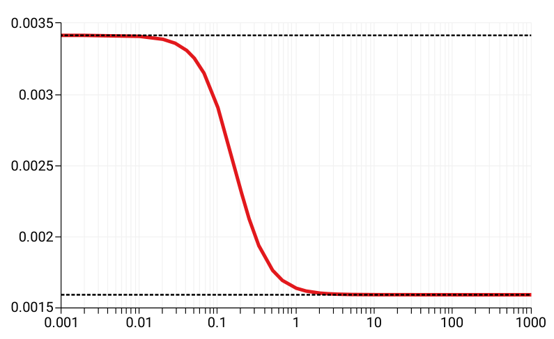
In the following, we will analyze the influence of a variation of the length-scale parameter $L_{\mathrm{c}}$ on the response of the relaxed micromorphic model for case A. The relation of the relaxed micromorphic model to the classical Cauchy theory has been discussed in detail in [40, 3] for the limiting case $L_{\mathrm{c}}\rightarrow 0$ and $L_{\mathrm{c}}\rightarrow\infty$. The case $L_{\mathrm{c}}\rightarrow 0$ relates to a macroscopic view on the material with microstructure, with the relaxed micromorphic model being equivalent to a linear elasticity model with stiffness $\mathbb{C}_{\mathrm{macro}}$ defined as the Reuss lower-bound of $\mathbb{C}_{\mathrm{e}}$ and $\mathbb{C}_{\mathrm{micro}}$, i.e. $\mathbb{C}_{\mathrm{macro}}:=(\mathbb{C}_{\mathrm{e}}^{-1}+\mathbb{C}_{\mathrm{micro}}^{-1})^{-1}$. The case $L_{\mathrm{c}}\rightarrow\infty$ resembles an infinite zoom into the material, where an equivalence to linear elasticity with $\mathbb{C}_{\mathrm{micro}}$ can be derived, cf. [40]. In the latter case, it can be shown that it holds that ${{\bm{P}}}=\nabla{{\bm{u}}}$. In our study, we approximate the limiting cases by $L_{\mathrm{c}}=10^{-3}$ and $L_{\mathrm{c}}=10^{3}$, respectively. Figure 12 shows the elastic energy $W$ along the radius and Figure 13 illustrates the non-vanishing components of ${{\bm{P}}}$ together with the respective displacement gradient components using 30624 Q2NQ2 elements. In Figure 14, we plot the total potential of the relaxed micromorphic model varying the characteristic length parameter $L_{\mathrm{c}}$. The figures clearly show the above described behavior. The bounded behavior of the relaxed micromorphic model for small sizes, i.e. $L_{\mathrm{c}}\rightarrow 0$, is an important advantage which most other generalized continua miss. For the linear elasticity model, a standard T2 nodal element is implemented.

Next, we investigate the behavior of the different stresses ${\bm{\sigma}}$, ${\bm{\sigma}}_{\textrm{micro}}$ and ${{\bm{m}}}$ under a variation of $L_{\mathrm{c}}$. The force stress tensor ${\bm{\sigma}}$ shown in Figure 15 vanishes for large value of the characteristic length, $L_{\mathrm{c}}=1000$, while it is bounded from above by the classical linear elasticity stress with elasticity tensor $\mathbb{C}_{\mathrm{macro}}$ for $L_{\mathrm{c}}=0.001$. The only non-vanishing component of the moment stress $m_{rz}$ is shown in Figure 16 ($m_{\theta z}=0$), which behaves opposite to the force stress when varying $L_{\mathrm{c}}$. It is nearly zero for $L_{\mathrm{c}}=0.001$ and it rises for growing $L_{\mathrm{c}}$. The micro-stress shown in Figure 17 is confined between the linear elasticity stress with elasticity tensor $\mathbb{C}_{\mathrm{micro}}$ from above and the one with $\mathbb{C}_{\mathrm{macro}}$ from below for large and small values of the characteristic length, respectively. Summarizing the previous findings shortly, increasing the characteristic length diminishes force stress and raises the micro- and moment stresses, while both force and moment stresses vanish for large and small values of the characteristic length, respectively, the micro-stress is always present.

References

- Aivaliotis et al. [2020] A. Aivaliotis, D. Tallarico, M. Valerio. d‘Agostino, A. Daouadji, P. Neff, and A. Madeo. Frequency- and angle-dependent scattering of a finite-sized meta-structure via the relaxed micromorphic model. Archive of Applied Mechanics, 90:1073–1096, 2020.
- Altan and Aifantis [1997] B. S. Altan and E. C. Aifantis. On some aspects in the special theory of gradient elasticity. Journal of the Mechanical Behavior of Materials, 8(3):231–282, 1997.
- Barbagallo et al. [2017] G. Barbagallo, A. Madeo, M. V. d’Agostino, R. Abreu, I.-D. Ghiba, and P. Neff. Transparent anisotropy for the relaxed micromorphic model: Macroscopic consistency conditions and long wave length asymptotics. International Journal of Solids and Structures, 120:7–30, 2017.
- Barbagallo et al. [2019] G. Barbagallo, D. Tallarico, M. V. d’Agostino, A. Aivaliotis, P. Neff, and A. Madeo. Relaxed micromorphic model of transient wave propagation in anisotropic band-gap metastructures. International Journal of Solids and Structures, 162:148–163, 2019.
- Boffi et al. [2014] D. Boffi, F. Brezzi, and M. Fortin. Mixed Finite Element Methods and Applications, volume 44 of Springer Series in Computational Mathematics. Springer, Berlin, Heidelberg, 2014.
- Brezzi et al. [1985] F. Brezzi, J. Douglas, and L. D. Marini. Two families of mixed finite elements for second order elliptic problems. Numerische Mathematik, 47:217–235, 1985.
- Cosserat and Cosserat [1909] E. Cosserat and F. Cosserat. Theory of deformable bodies. Hermann and Sons, 1909.
- Crowley et al. [1988] C. W. Crowley, P. P. Silvester, and H. Hurwitz. Covariant projection elements for 3d vector field problems. IEEE Transactions on Magnetics, 24(1):397–400, 1988.
- d‘Agostino et al. [2020] M. V. d‘Agostino, G. Barbagallo, I.-D. Ghiba, B. Eidel, P. Neff, and A. Madeo. Effective description of anisotropic wave dispersion in mechanical band-gap metamaterials via the relaxed micromorphic model. Journal of Elasticity, 139:299–329, 2020.
- d’Agostino et al. [2021] M. V. d’Agostino, G. Rizzi, H. Khan, P. Lewintan, A. Madeo, and P. Neff. The consistent coupling boundary condition for the classical micromorphic model: existence, uniqueness and interpretation of the parameters (submitted), 2021.
- Eringen [1968] A. C. Eringen. Mechanics of micromorphic continua. In Mechanics of Generalized Continua, pages 18–35. Springer, Berlin, Heidelberg., 1968.
- Eringen and Suhubi [1964] A. C. Eringen and E. S. Suhubi. Nonlinear theory of simple micro-elastic solids-I. International Journal of Engineering Science, 2(2):189–203, 1964.
- Fischer et al. [2011] P. Fischer, M. Klassen, J. Mergheim, P. Steinmann, and R. Müller. Isogeometric analysis of 2d gradient elasticity. Computational Mechanics, 47:1432–0924, 2011.
- Fischer et al. [2020] S. C. L. Fischer, L. Hillen, and C. Eberl. Mechanical metamaterials on the way from laboratory scale to industrial applications: Challenges for characterization and scalability. Materials, 13(16), 2020.
- Ghiba et al. [2015] I.-D. Ghiba, P. Neff, A. Madeo, L. Placidi, and G. Rosi. The relaxed linear micromorphic continuum: existence, uniqueness and continuous dependence in dynamics. Mathematics and Mechanics of Solids, 20(10):1171–1197, 2015.
- Jiang and Li [2018] Y. Jiang and Y. Li. 3d printed auxetic mechanical metamaterial with chiral cells and re-entrant cores. Scientific reports, 8(1):2397, 2018.
- Kirby et al. [2012] R. C. Kirby, A. Logg, M. E. Rognes, and A. R. Terrel. Common and unusual finite elements. In Automated Solution of Differential Equations by the Finite Element Method: The FEniCS Book, pages 95–119. Springer Berlin Heidelberg, Berlin, Heidelberg, 2012.
- Korelc and Wriggers [2016] J. Korelc and P. Wriggers. Automation of Finite Element Methods. Springer International Publishing, 2016.
- Lee et al. [2012] J.-H. Lee, J. P. Singer, and E. L. Thomas. Micro-/nanostructured mechanical metamaterials. Advanced Materials, 24(36):4782–4810, 2012.
- Lei et al. [2019] M. Lei, W. Hong, Z. Zhao, C. Hamel, M. Chen, H. Lu, and H. J. Qi. 3d printing of auxetic metamaterials with digitally reprogrammable shape. ACS Applied Materials & Interfaces, 11(25):22768–22776, 2019.
- Leismann and Mahnken [2015a] T. Leismann and R. Mahnken. Comparison of hyperelastic micromorphic, micropolar and microstrain continua. International Journal of Non-Linear Mechanics, 77:115–127, 2015a.
- Leismann and Mahnken [2015b] T. Leismann and R. Mahnken. Transition from hyperelastic micromorphic to micropolar and microstrain continua. PAMM, 15(1):329–330, 2015b.
- Madeo et al. [2015a] A. Madeo, P. Neff, I.-D. Ghiba, L. Placidi, and G. Rosi. Band gaps in the relaxed linear micromorphic continuum. Zeitschrift für angewandte Mathematik und Mechanik, 95(9):880–887, 2015a.
- Madeo et al. [2015b] A. Madeo, P. Neff, I. D. Ghiba, L. Placidi, and G. Rosi. Wave propagation in relaxed micromorphic continua: modeling metamaterials with frequency band-gaps. Continuum Mechanics and Thermodynamics, 75:551–571, 2015b.
- Madeo et al. [2016a] A. Madeo, P. Neff, M. V. d’Agostino, and G. Barbagallo. Complete band gaps including non-local effects occur only in the relaxed micromorphic model. Comptes Rendus Mécanique, 344(11-12):784–796, 2016a.
- Madeo et al. [2016b] A. Madeo, P. Neff, I.-D. Ghiba, and G. Rosi. Reflection and transmission of elastic waves in non-local band-gap metamaterials: a comprehensive study via the relaxed micromorphic model. Journal of the Mechanics and Physics of Solids, 95:441–479, 2016b.
- Madeo et al. [2017] A. Madeo, P. Neff, G. Barbagallo, M. V. d’Agostino, and I.-D.l Ghiba. A review on wave propagation modeling in band-gap metamaterials via enriched continuum models. In Mathematical Modelling in Solid Mechanics, volume 69 of Adv. Struct. Mater., pages 89–105. Springer, Singapore, 2017.
- Madeo et al. [2018] A. Madeo, M. Collet, M. Miniaci, K. Billon, M. Ouisse, and P. Neff. Modeling phononic crystals via the weighted relaxed micromorphic model with free and gradient micro-inertia. Journal of Elasticity, 130(1):59–83, 2018.
- Mindlin [1964] R. D Mindlin. Micro-structure in linear elasticity. Archive for Rational Mechanics and Analysis, 16:51–78, 1964.
- Mindlin and Eshel [1968] R. D. Mindlin and N. N. Eshel. On first strain-gradient theories in linear elasticity. International Journal of Solids and Structures, 4(1):109–124, 1968. ISSN 0020-7683.
- Monk [1993] P. Monk. An analysis of Nédélec’s method for the spatial discretization of maxwell’s equations. Journal of Computational and Applied Mathematics, 47(1):101–121, 1993.
- Montgomery et al. [2020] S. M. Montgomery, X. Kuang, C. D. Armstrong, and H. J. Qi. Recent advances in additive manufacturing of active mechanical metamaterials. Current Opinion in Solid State and Materials Science, 24(5):100869, 2020.
- Nédélec [1980] J. C. Nédélec. Mixed finite elements in R3. Numerische Mathematik, 35(3):315–341, 1980.
- Nédélec [1986] J. C. Nédélec. A new family of mixed finite elements in R3. Numerische Mathematik, 50:57–81, 1986.
- Neff [2006] P. Neff. The Cosserat couple modulus for continuous solids is zero viz the linearized cauchy-stress tensor is symmetric. ZAMM - Journal of Applied Mathematics and Mechanics / Zeitschrift für Angewandte Mathematik und Mechanik, 86(11):892–912, 2006.
- Neff et al. [2010] P. Neff, J. Jeong, I. Münch, and H Ramézani. Linear Cosserat elasticity, conformal curvature and bounded stiffness. In Mechanics of Generalized Continua: One Hundred Years After the Cosserats, pages 55–63. Springer New York, 2010.
- Neff et al. [2014] P. Neff, I.-D. Ghiba, A. Madeo, L. Placidi, and G. Rosi. A unifying perspective: the relaxed linear micromorphic continuum. Continuum Mechanics and Thermodynamics, 26(5):639–681, 2014.
- Neff et al. [2015] P. Neff, I. D. Ghiba, M. Lazar, and A. Madeo. The relaxed linear micromorphic continuum: well-posedness of the static problem and relations to the gauge theory of dislocations. The Quarterly Journal of Mechanics and Applied Mathematics, 68(1):53–84, 2015.
- Neff et al. [2017] P. Neff, A. Madeo, G. Barbagallo, M. V. d’Agostino, R. Abreu, and I.-D. Ghiba. Real wave propagation in the isotropic-relaxed micromorphic model. Proceedings of the Royal Society A: Mathematical, Physical and Engineering Sciences, 473(2197):20160790, 2017.
- Neff et al. [2020] P. Neff, B. Eidel, M. V. d‘Agostino, and A. Madeo. Identification of scale-independent material parameters in the relaxed micromorphic model through model-adapted first order homogenization. Journal of Elasticity, 139:269–298, 2020.
- Olm et al. [2019] M. Olm, S. Badia, and A. F. Martín. On a general implementation of h- and p-adaptive curl-conforming finite elements. Advances in Engineering Software, 132:74–91, 2019.
- Plocher and Panesar [2019] J. Plocher and A. Panesar. Review on design and structural optimisation in additive manufacturing: Towards next-generation lightweight structures. Materials and Design, 183:108164, 2019.
- Raviart and Thomas [1977] P. A. Raviart and J. M. Thomas. A mixed finite element method for 2-nd order elliptic problems. In I. Galligani and E. Magenes, editors, Mathematical Aspects of Finite Element Methods, pages 292–315, Berlin, Heidelberg, 1977. Springer Berlin Heidelberg.
- Rizzi et al. [2021a] G. Rizzi, G. Hütter, H. Khan, I.-D. Ghiba, A. Madeo, and P. Neff. Analytical solution of the cylindrical torsion problem for the relaxed micromorphic continuum and other generalized continua (including full derivations). to appear in Mathematics and Mechanics of Solids, 2021a.
- Rizzi et al. [2021b] G. Rizzi, G. Hütter, A. Madeo, and P. Neff. Analytical solutions of the simple shear problem for micromorphic models and other generalized continua. Archive of Applied Mechanics, 91:2237–2254, 2021b.
- Rizzi et al. [2021c] G. Rizzi, G. Hütter, A. Madeo, and P. Neff. Analytical solutions of the cylindrical bending problem for the relaxed micromorphic continuum and other generalized continua. Continuum Mechanics and Thermodynamics, 33:1505–1539, 2021c.
- Rizzi et al. [2021d] G. Rizzi, H. Khan, I.-D. Ghiba, A. Madeo, and P. Neff. Analytical solution of the uniaxial extension problem for the relaxed micromorphic continuum and other generalized continua (including full derivations). to appear in Archive of Applied Mechanics, 2021d.
- Rognes et al. [2009] M. E. Rognes, R. C. Kirby, and A. Logg. Efficient assembly of and conforming finite elements. SIAM Journal on Scientific Computing, 31(9):4130–4151, 2009.
- Schöberl and Zaglmayr [2005] J. Schöberl and S. Zaglmayr. High order Nédélec elements with local complete sequence properties. The International Journal for Computation and Mathematics in Electrical and Electronic Engineering, 24(2):374–384, 2005.
- Sky et al. [2021] A. Sky, M. Neunteufel, I. Münch, J. Schöberl, and P. Neff. A hybrid finite element formulation for a relaxed micromorphic continuum model of antiplane shear. Computational Mechanics, 68:1–24, 2021.
- Suhubi and Eringen [1964] E. S. Suhubi and A. C. Eringen. Nonlinear theory of micro-elastic solids-II. International Journal of Engineering Science, 2(4):389–404, 1964.
- Surjadi et al. [2019] J. U. Surjadi, L. Gao, H. Du, X. Li, X. Xiong, N. X. Fang, and Y. Lu. Mechanical metamaterials and their engineering applications. Advanced Engineering Materials, 21(3):1800864, 2019.
- Wriggers [2008] P. Wriggers. Nonlinear Finite Element Methods. Springer, Berlin, Heidelberg, 2008.
- Yu et al. [2018] X. Yu, J. Zhou, H. Liang, Z. Jiang, and L. Wu. Mechanical metamaterials associated with stiffness, rigidity and compressibility: A brief review. Progress in Materials Science, 94:114–173, 2018.
- Zadpoor [2016] A. A. Zadpoor. Mechanical meta-materials. Materials Horizons, 3:371–381, 2016.
Appendix A Appendix
A.1 Construction of triangular Nédélec shape functions
The parameter elements are defined in the natural coordinates . Triangular elements are defined on the domain . The finite elements with edge numbering are shown in Figure 1.
A.1.1 . First-order triangular element NT1
The Nédélec space of this element reads