跳到论文正文
W Papers独立论文阅读器 arXiv:2112.00165 论文正文 计算阅读时间 · 0%
引用这篇论文根据当前论文元数据生成,正式投稿前建议核对。


License: arXiv.org perpetual non-exclusive license
arXiv:2112.00165v5 [cs.RO] 13 Jan 2023

Coordinated Multi-Robot Trajectory Tracking Control
over Sampled Communicationfootnoteinfo

Enrica Rossi Email: renrica91@gmail.com    Marco Tognon Email: marco.tognon@inria.fr    Luca Ballotta Email: ballotta@dei.unipd.it    Ruggero Carli Email: carlirug@dei.unipd.it    Juan Cortés Email: juan.cortes@laas.fr    Antonio Franchi Email: a.franchi@utwente.nl    Luca Schenato Email: schenato@dei.unipd.it
Abstract

In this paper, we propose an inverse-kinematics controller for a class of multi-robot systems in the scenario of sampled communication. The goal is to make a group of robots perform trajectory tracking in a coordinated way when the sampling time of communications is much larger than the sampling time of low-level controllers, disrupting theoretical convergence guarantees of standard control design in continuous time. Given a desired trajectory in configuration space which is pre-computed offline, the proposed controller receives configuration measurements, possibly via wireless, to re-compute velocity references for the robots, which are tracked by a low-level controller. We propose joint design of a sampled proportional feedback plus a novel continuous-time feedforward that linearizes the dynamics around the reference trajectory: this method is amenable to distributed communication implementation where only one broadcast transmission is needed per sample. Also, we provide closed-form expressions for instability and stability regions and convergence rate in terms of proportional gain kk and sampling period TT. We test the proposed control strategy via numerical simulations in the scenario of cooperative aerial manipulation of a cable-suspended load using a realistic simulator (Fly-Crane). Finally, we compare our proposed controller with centralized approaches that adapt the feedback gain online through smart heuristics, and show that it achieves comparable performance.

keywords
Control over sampled communications; distributed control; multi-robot systems; trajectory tracking; UAVs.
††thanks: [††address: Mas Automazioni S.r.l., Torre di Mosto, Italy††address: Inria, Université de Rennes, CNRS, IRISA, Rennes, France††address: Department of Information Engineering, University of Padova, Italy††address: LAAS-CNRS, Université de Toulouse, CNRS, Toulouse, France††address: Robotics and Mechatronics lab, University of Twente, Enschede, The Netherlands

footnoteinfo]This work Partially funded by: the European Commission project H2020 AERIAL-CORE (EC 871479), the ANR, Project ANR-17- CE33-0007 MuRoPhen and by University of Padova grant “Magic” SCHE_SID17_01.

, , , , , ,

This article has been accepted for publication on Automatica.Please cite the paper as: E. Rossi, M. Tognon, L. Ballotta, R. Carli, J. Cortés, A. Franchi, and L. Schenato,"Coordinated Multi-Robot Trajectory Tracking Control over Sampled Communication”,Automatica (to appear).

1 Introduction

Unmanned Aerial Vehicles (UAVs) are used in the context of mobile robotics to perform surveillance, coverage, exploration, and transportation [18]. Generally speaking, a group of robots allows to improve task performance with respect to (w.r.t.) the single-robot solution. Multiple robots can mitigate problems such as limited payload and time of flight [2]. However, they require careful consideration of cooperation or coordination strategies to achieve common goals [6]. Consider a group of UAVs that transports a load while avoiding obstacles. In this case, not only each UAV needs to avoid obstacles, but the overall multi-robot system should move in a way such that the load avoids obstacles, as well [4].

One of the most direct approaches to control multi-robot systems is the centralized kinematic/dynamic inversion [31, 17, 16, 26, 1]. Because of its nature, failure of the central unit may cause the whole task to fail. Distributed and decentralized approaches spread computations across the robots, guaranteeing greater robustness and flexibility w.r.t. a centralized one [25]. Although such approaches are preferable for multi-robot systems, they often lack global information such as load state and parameters, or the total number of robots. This aspect increases the difficulty of the controller design and might even degrade performance. Examples of distributed control methods, where robots explicitly exchange local data, can be found for groups of ground [20, 5, 10, 22], underwater [3, 30], and aerial robots [19]. Conversely, decentralized control strategies allow for no direct communication among robots, with examples including ground or aerial manipulators [29, 36]. Also, to reduce communication issues, communication-less approaches relying on a leader-follower paradigm were presented for cooperative transportation and manipulation [11, 33, 37, 7, 35]. In these cases, communication is implicitly given by forces exerted on the load [34]. However, force feedback may be insufficient for precise tracking, because it lacks pose information. The latter can be retrieved by communication among robots, e.g., making them exchange poses, or installing a sensor on the load to broadcast its pose. This setup can also be extended to formation control problems where a group of robots needs to complete a task [8, 9]. For example, a common goal is mapping or surveillance of an area while robots keep a certain 3D formation in order to, e.g., minimize overlaps among their fields of view [27]. In this case, communication-based approaches let robots exchange group-level measurements, such as relative distances.

In applications, limited bandwidth of wireless channels disrupts the assumption of continuous-measurement feedback. As so, specific strategies are needed to deal with sampled communication [15, 12, 32]. However, little work is currently available for multi-robot manipulation.

1.1 Preview of Key Results

Refer to caption
Figure 1: We propose a controller for trajectory tracking when measurements are transmitted every TT seconds, with feedback proportional gain kk. We show that, if (k,T)(k,T) lies outside the dashed red curve, the tracking error is not ρ\rho-monotonically contractive, while zero tracking error is guaranteed if (k,T)(k,T) lies below the solid green curve τs​(k)\tau_{s}(k). In particular, there exist sampling time Tm​a​xT_{max} such that no gain kk can guarantee convergence if T>Tm​a​xT>T_{max} and sampling time τC​R\tau_{CR} such that a stabilizing gain exists for any T<τC​RT<\tau_{CR}.

In this paper, we aim to design a multi-robot distributed communication controller for trajectory tracking when wireless communication induces non-negligible sampling of feedback measurements. In this context, a distributed implementation is preferred because (i) it reduces the overall communication burden and related issues such as packet loss or latency and (ii) it enhances system robustness and scalability. Inspired by previous work [24] where point-stabilization was considered, we propose a novel Sampled communication-aware Inverse-Kinematic controller for Multi-robot systems (SIKM) to address the problem of trajectory tracking under sampled communication. Our contributions are summarized as follows.

  • •

    We develop a distributed SIKM controller for trajectory tracking that receives sampled measurements and re-computes reference robot velocities along the trajectory, exploiting a novel continuous-time feedforward term that allows exact trajectory tracking even in the presence of sampled communication.

  • •

    We show that, differently from [24], there are a maximum sampling time Tm​a​xT_{max} and a minimum feedback gain km​i​nk_{min} beyond which trajectory tracking cannot be achieved, as graphically depicted in red in Fig. 1.

  • •

    We provide closed-form expressions, whose coefficients can be numerically computed, for the stability region (depicted in green in Fig. 1) and for the (exponential) convergence rate of the trajectory tracking error norm in terms of communication sampling period TT and feedback gain kk. We consider stability in terms of ρ\rho-monotonic contractiveness, which, roughly speaking, ensures that the trajectory monotonically decreases the tracking error overtime in the absence of external disturbances and is bounded away from singularities.

  • •

    We validated our strategy by testing the controller on a realistic dynamical simulator which replicates with high accuracy the experimental setup available at LAAS-CNRS Lab, Fly-Crane [26], including dynamical inertial terms, motor actuators, sensor noise, and real-time embedded software implementation.

1.2 Paper Outline

In Section 2 we introduce the class of considered multi-robot systems, provide the kinematic model (Section 2.1), and give an example of real system (Section 2.2). In Section 3 we review control architectures for trajectory tracking, and present our proposed SIKM controller in Section 3.1. In Section 4 we derive fundamental stability limitations in terms of feedback gain and sampling time. In Section 5 we compute an upper bound for the convergence rate, outline a numerical procedure to estimate it from data (Section 5.1), and explicitly find controller parameters that yield the fastest convergence (Section 5.2). In Section 6 we test our controller on a realistic simulator of the Fly-Crane, showing that it outperforms standard designs under sampled communication. Final remarks are drawn in Section 7.

2 System Model and Problem Formulation

2.1 Kinematics of Multi-Robot Systems

In this section, we describe the kinematic model of a multi-robot system composed of NN robots that exchange state information with a common pivot, labeled as VV, to fulfill a task. As so, robots need not communicate among themselves, but they implicitly coordinate their motions by communicating with the pivot. The pivot may be an object to be manipulated, a robot to be escorted, or a vehicle in the space. The kinematic model is given by

[𝐩1​…​𝐩N]⊤=𝐡⁡(𝐪)=[𝐡(1)​(𝐪1,𝐪V)​…​𝐡(N)​(𝐪N,𝐪V)]⊤.\displaystyle\scalebox{.9}{$\begin{bmatrix}\mathbf{p}_{1}\;\,\dots\;\,\mathbf{p}_{N}\end{bmatrix}$}^{\top}=\mathbf{h(q)}=\scalebox{.9}{$\begin{bmatrix}\mathbf{h}^{(1)}(\mathbf{q}_{1},\mathbf{q}_{V})\;\,\dots\,\;\mathbf{h}^{(N)}(\mathbf{q}_{N},\mathbf{q}_{V})\end{bmatrix}$}^{\top}.

This function maps the Lagrangian coordinates of the system 𝐪=[𝐪1⊤⋯𝐪N⊤𝐪V⊤]⊤∈ℝm\mathbf{q}=[\mathbf{q}_{1}^{\top}\,\cdots\,\mathbf{q}_{N}^{\top}\ \mathbf{q}_{V}^{\top}]^{\top}\in\mathbb{R}^{m} to the vector collecting the robots configurations 𝐩=[𝐩1⊤​…​𝐩N⊤]⊤∈ℝn\mathbf{p}=\scalebox{.9}{$\begin{bmatrix}\mathbf{p}_{1}^{\top}\;\,\dots\;\,\mathbf{p}_{N}^{\top}\end{bmatrix}$}^{\top}\in\mathbb{R}^{n}. In particular, 𝐩i∈ℝni\mathbf{p}_{i}\in\mathbb{R}^{n_{i}} is the position of the iith robot in space, 𝐪i∈ℝmi\mathbf{q}_{i}\in\mathbb{R}^{m_{i}} gathers the angles and/or distances between the pivot VV and the iith robot, and 𝐪V∈ℝmV\mathbf{q}_{V}\in\mathbb{R}^{m_{V}} represents the pose (position and orientation) of the pivot. Notice that m=∑i=1Nmi+mVm=\sum_{i=1}^{N}{m_{i}}+m_{V} and n=∑i=1Nnin=\sum_{i=1}^{N}{n_{i}}. The differential kinematics of the system is

𝐩˙\displaystyle\dot{\mathbf{p}} =𝐀𝐪​𝐪˙,\displaystyle=\mathbf{A_{q}}\,\,\dot{\mathbf{q}}, (1)

where the Jacobian 𝐀𝐪=∂𝐡⁡(𝐪)∂𝐪∈ℝn×m\mathbf{A_{q}}=\frac{\partial\mathbf{h(q)}}{\partial\mathbf{q}}\in\mathbb{R}^{n\times m} has structure

𝐀𝐪=[𝐀𝐪1(1)𝟎𝐀𝐪V(1)⋱⋮𝟎𝐀𝐪N(N)𝐀𝐪V(N)],\displaystyle\mathbf{A_{q}}=\scalebox{.9}{$\begin{bmatrix}\begin{array}[]{ccc|c}\mathbf{A}^{(1)}_{\mathbf{q}_{1}}&&\text{$\mathbf{0}$}&\mathbf{A}^{(1)}_{\mathbf{q}_{V}}\\ &\ddots&&\vdots\\ \text{$\mathbf{0}$}&&\mathbf{A}^{(N)}_{\mathbf{q}_{N}}&\mathbf{A}^{(N)}_{\mathbf{q}_{V}}\end{array}\end{bmatrix}$}, (2)

𝐀𝐪i(i)=∂𝐡(i)​(𝐪i,𝐪V)∂𝐪i∈ℝni×mi\mathbf{A}^{(i)}_{\mathbf{q}_{i}}=\frac{\partial\mathbf{h}^{(i)}(\mathbf{q}_{i},\mathbf{q}_{V})}{\partial\mathbf{q}_{i}}\in\mathbb{R}^{n_{i}\times m_{i}} and 𝐀𝐪V(i)=∂𝐡(i)​(𝐪i,𝐪V)∂𝐪V∈ℝni×mV\mathbf{A}^{(i)}_{\mathbf{q}_{V}}=\frac{\partial\mathbf{h}^{(i)}(\mathbf{q}_{i},\mathbf{q}_{V})}{\partial\mathbf{q}_{V}}\in\mathbb{R}^{n_{i}\times m_{V}}. We focus on the case n=mn=m, corresponding to square systems. Let us make an example to justify this choice. Consider the multi-robot system in Fig. , where robots are linked to a platform though rigid cables, and assume that 𝐀𝐪\mathbf{A_{q}} is invertible and that desired robot velocities 𝐩˙d\mathbf{\dot{p}}^{d} are assigned a priori. In this case, there always exists a vector 𝐪˙=𝐀𝐪−1​𝐩˙d\mathbf{\dot{q}}=\mathbf{A}^{-1}_{\mathbf{q}}\mathbf{\dot{p}}^{d} in configuration space that allows the robots to achieve the desired velocity. The next section expands this example more in details. If n≠mn\neq m, the Jacobian is not square. In particular, the system is redundant if n>mn>m. If n<mn<m, there exist trajectories 𝐪˙\mathbf{\dot{q}} in the configuration space which are infeasible for any input 𝐩˙d\mathbf{\dot{p}}^{d}. Such cases require a dedicated analysis which goes beyond the scope of this paper. We refer to the preprint [23] for such an analysis, that, with some attention, allows to integrate the control strategy studied here into more general systems.

Furthermore, we consider a cascade control architecture where we design the proposed SIKM controller at the kinematic level. The latter provides the desired motor velocities which are tracked by low-level dynamics controllers (see Fig. 4), assuming that these have larger closed-loop bandwidth than the SIKM. This assumption is indeed validated by extensive simulations of the proposed architecture on a full dynamical model (including low-level dynamics as well as external disturbances) with a realistic simulator of the testbed Fly-Crane.

2.2 Examples of Square Systems

Refer to caption
(a)
Refer to caption
(b)
Refer to caption
(c)
Refer to caption
(d)
Figure 2: Square systems where a common object is manipulated by a group of UAVs. All the possible combinations of (N1​c,N2​c,N)(N_{1c},N_{2c},N) introduced in Sec. 2.2 are represented.

In the literature, we can find several examples of square systems. One is the multi-robot system depicted in Fig.  (called Fly-Crane [16]), where three UAVs transport a common platform. Each robot is linked to the load through two rigid cables. The generalized coordinates are chosen as 𝐪=[q1​q2​q3​𝐪V⊤]⊤\mathbf{q}=[q_{1}\,\,q_{2}\,\,q_{3}\,\,\mathbf{q}_{V}^{\top}]^{\top}. The robot positions 𝐩i∈ℝ3\mathbf{p}_{i}\,\in\mathbb{R}^{3} are collected in the vector 𝐩=[𝐩1⊤​𝐩2⊤​𝐩3⊤]⊤\mathbf{p}=[\mathbf{p}_{1}^{\top}\,\,\mathbf{p}_{2}^{\top}\,\,\mathbf{p}_{3}^{\top}]^{\top}. Thus, the velocity vectors 𝐪˙,𝐩˙∈ℝ9\mathbf{\dot{q}},\,\mathbf{\dot{p}}\in\mathbb{R}^{9} have the same dimension and 𝐀𝐪∈ℝ9×9\mathbf{A_{q}}\,\in\mathbb{R}^{9\times 9} is a square matrix. However, this is a particular case of a larger class: different square systems can be obtained by simply changing the number of robots transporting the platform or the number of cables linking each robot to it. Notice that if one cable was used instead of two, as shown in Fig. , then 𝐪i=[qi1​qi2]⊤∈ℝ2\mathbf{q}_{i}=[q_{i_{1}}\ q_{i_{2}}]^{\top}\in\mathbb{R}^{2} because each cable can move in two directions (assuming that movements about the cable axis are not allowed). In this case, the system is no more guaranteed to be square. In particular, it holds n=3​Nn=3N and m=6+2​N1​c+N2​cm=6+2N_{1c}+N_{2c} where N1​c≥0N_{1c}\geq 0 is the number of robots linked to the load through one cable and N2​c≥0N_{2c}\geq 0 indicates the number of robots linked through two cables. We have that N=N1​c+N2​cN=N_{1c}+N_{2c} and, for a square system n=mn=m, it must be 3​N=6+2​N1​c+N2​c3N=6+2N_{1c}+N_{2c}. From these relations it turns out that N2​c≤3N_{2c}\leq 3, N1​c≤6N_{1c}\leq 6 and N≤6N\leq 6; in particular, the possible configurations (N1​cN_{1c},N2​cN_{2c},NN) are: (0,3,3) in Fig. , (2,2,4) in Fig. , (4,1,5) in Fig. , (6,0,6) in Fig. .

Refer to caption
Figure 3: Representation of a multi-robot system where three robots must keep the same orientation φi\varphi_{i} w.r.t. the reference frame centered in the point OcO_{c} during the assigned task.

Other examples of square systems are found in the context of formation control problems [9], as the one represented in Fig. 3. Three ground robots move in a 2-dimensional space while respecting some constraints w.r.t. the frame ℱV={OV,𝐱V,𝐲V}\mathcal{F}_{V}=\{O_{V},\mathbf{x}_{V},\mathbf{y}_{V}\} representing the pivot (e.g., the barycenter of the system). The position PiP_{i} of each robot, defined by the vector 𝐩i=[xi​yi]⊤\mathbf{p}_{i}=[x_{i}\;\,y_{i}]^{\top}, is described as a function of: the pivot position 𝐩V=[xV​yV]⊤\mathbf{p}_{V}=[x_{V}\,\;y_{V}]^{\top}, the distance did_{i} from PiP_{i} to OVO_{V}, the angle φi\varphi_{i} between the line OV−PiO_{V}-P_{i} and the axis 𝐱V\mathbf{x}_{V}, and the angle φV\varphi_{V} between 𝐱V\mathbf{x}_{V} and 𝐱W\mathbf{x}_{W} of the world reference frame ℱW={OW,𝐱W,𝐲W}\mathcal{F}_{W}=\{O_{W},\mathbf{x}_{W},\mathbf{y}_{W}\}. It is trivial to express the position PiP_{i} w.r.t. ℱW\mathcal{F}_{W}:

𝐩i=𝐡⁡(𝐪i,𝐪V),\mathbf{p}_{i}=\mathbf{h}(\mathbf{q}_{i},\mathbf{q}_{V}),

where 𝐪i=[di​φi]⊤∈ℝ2\mathbf{q}_{i}=[d_{i}\ \varphi_{i}]^{\top}\in\mathbb{R}^{2}, 𝐪V=[xV​yV​φV]⊤∈ℝ3\mathbf{q}_{V}=[x_{V}\ y_{V}\ \varphi_{V}]^{\top}\in\mathbb{R}^{3} and

𝐡⁡(𝐪i,𝐪V)=[xVyV]+[cos⁡(φV)−sin⁡(φV)sin⁡(φV)cos⁡(φV)]​[di​cos⁡(φi)di​sin⁡(φi)].\mathbf{h}(\mathbf{q}_{i},\mathbf{q}_{V})=\begin{bmatrix}x_{V}\\ y_{V}\end{bmatrix}+\begin{bmatrix}\cos(\varphi_{V})\ \ -\sin(\varphi_{V})\\ \sin(\varphi_{V})\ \ \cos(\varphi_{V})\end{bmatrix}\begin{bmatrix}d_{i}\,\cos(\varphi_{i})\\ d_{i}\,\sin(\varphi_{i})\end{bmatrix}.

Let us define the vector of robot positions as 𝐩=[𝐩1⊤​𝐩2⊤​𝐩3⊤]⊤∈ℝ6\mathbf{p}=[\mathbf{p}_{1}^{\top}\ \mathbf{p}_{2}^{\top}\ \mathbf{p}_{3}^{\top}]^{\top}\in\mathbb{R}^{6} and the vector of generalized coordinates as 𝐪=[𝐪1⊤​𝐪2⊤​𝐪3⊤​𝐪V⊤]⊤∈ℝ9\mathbf{q}=[\mathbf{q}_{1}^{\top}\ \mathbf{q}_{2}^{\top}\ \mathbf{q}_{3}^{\top}\ \mathbf{q}_{V}^{\top}]^{\top}\in\mathbb{R}^{9}. Hence, we can write 𝐡⁡(𝐪)​=def​[𝐡​(𝐪1,𝐪V)⊤​𝐡​(𝐪2,𝐪V)⊤​𝐡​(𝐪3,𝐪V)⊤]⊤\mathbf{h(q)}\overset{\text{def}}{=}[\mathbf{h}(\mathbf{q}_{1},\mathbf{q}_{V})^{\top}\ \mathbf{h}(\mathbf{q}_{2},\mathbf{q}_{V})^{\top}\ \mathbf{h}(\mathbf{q}_{3},\mathbf{q}_{V})^{\top}]^{\top}. We assume that the robots must perform a task while keeping the angles φi\varphi_{i} constant w.r.t. ℱV\mathcal{F}_{V}, hence the differential kinematic model is:

𝐩˙=𝐀𝐪​𝐪˙′,\mathbf{\dot{p}}=\mathbf{A_{q}}\mathbf{\dot{q}}^{\prime},

where 𝐪˙′=[𝐪˙V⊤​d˙1​d˙2​d˙3]⊤\mathbf{\dot{q}}^{\prime}=[\dot{\mathbf{q}}_{V}^{\top}\,\;\dot{d}_{1}\,\;\dot{d}_{2}\,\;\dot{d}_{3}]^{\top} and

𝐀𝐪=[∂𝐡⁡(𝐪)∂𝐪V​∂𝐡⁡(𝐪)∂d1​∂𝐡⁡(𝐪)∂d2​∂𝐡⁡(𝐪)∂d3]∈ℝ6×6,\displaystyle\mathbf{A_{q}}=\left[\frac{\partial\mathbf{h}(\mathbf{q})}{\partial\mathbf{q}_{V}}\;\,\frac{\partial\mathbf{h}(\mathbf{q})}{\partial d_{1}}\;\,\frac{\partial\mathbf{h}(\mathbf{q})}{\partial d_{2}}\;\,\frac{\partial\mathbf{h}(\mathbf{q})}{\partial d_{3}}\right]\,\in\,\mathbb{R}^{6\times 6},

is a square matrix, hence this system is square, too.

The previous examples show that the considered class of square systems includes many relevant applications.

3 Control Architectures
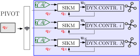
(a) Decentralized (no communication) control (4).
Refer to caption
(b) Distributed communication control (5).
Refer to caption
(c) Centralized communication control (6).
Figure 4: Controller architectures for trajectory tracking. The pivot is colored in gray, each robot (equipped with a dynamical controller which converts 𝐮\mathbf{u} to forces) in blue, sensor measurements in red, and the reference trajectory in green. The wireless symbol refers to sampled communication.

We consider a tracking problem where a multi-robot system is required to follow a sequence of desired configurations assigned a priori. We assume that such reference trajectory is generated offline by a high-level planner that takes into account goals such as obstacle avoidance, singular points, and energy minimization. Also, we assume that robots are equipped with dynamical controllers sufficiently fast w.r.t. the dynamics of the system, such that (s.t.) their velocities are fully controllable,

𝐩˙​(t)=𝐮​(t),\displaystyle\dot{\mathbf{p}}(t)=\mathbf{u}(t), (3)

where 𝐮=[𝐮1⊤⋯𝐮N⊤]⊤∈ℝn\mathbf{u}=[\mathbf{u}_{1}^{\top}\cdots\mathbf{u}_{N}^{\top}]^{\top}\in\mathbb{R}^{n}. We now enumerate possible control architectures to achieve trajectory tracking.

Decentralized (no communication) control. A commonly adopted architecture is the following fully decentralized controller,

𝐮i​(t)=κidec​(𝐩i​(t),𝐩ir​(t),𝐩˙ir​(t)).\mathbf{u}_{i}(t)=\kappa_{i}^{\text{dec}}\left(\mathbf{p}_{i}(t);\mathbf{p}_{i}^{r}(t),\mathbf{\dot{p}}_{i}^{r}(t)\right). (4)

In this case, each robot needs only local position measurements 𝐩i​(t)\mathbf{p}_{i}(t) (no configuration variables 𝐪⁡(t)\mathbf{q}(t) are needed) to implement feedback and follow its reference trajectory (𝐩ir​(t),𝐩˙ir​(t))(\mathbf{p}_{i}^{r}(t),\mathbf{\dot{p}}_{i}^{r}(t)), namely, controller (4) is communication-less and the control design reduces to a distributed planning problem (Fig. 4a). A typical example is 𝐮i​(t)=−k⁡(𝐩i​(t)−𝐩ir​(t))+𝐩˙ir​(t)\mathbf{u}_{i}(t)=-k(\mathbf{p}_{i}(t)-\mathbf{p}_{i}^{r}(t))+\mathbf{\dot{p}}_{i}^{r}(t). However, lacking communication and coordination, strategy (4) is not robust against disturbances or robot failures/biases.

Distributed communication control. A distributed controller reads

𝐮i​(t)=κidistr​(𝐪i​(t),𝐪V​(h​T),𝐪ir​(t),𝐪Vr​(t),𝐪˙ir​(t),𝐪˙Vr​(t)),\mathbf{u}_{i}(t)=\kappa_{i}^{\text{distr}}(\mathbf{q}_{i}(t),\mathbf{q}_{V}({{\color[rgb]{0,0,0}hT}});\mathbf{q}^{r}_{i}(t),\mathbf{q}^{r}_{V}(t),\mathbf{\dot{q}}^{r}_{i}(t),\mathbf{\dot{q}}^{r}_{V}(t)), (5)

where t∈[h​T,(h+1)​T)t\in[hT,(h+1)T), h∈ℕh\in\mathbb{N}. Specifically, 𝐮i​(t)\mathbf{u}_{i}(t) depends on the robot’s own configuration 𝐪i​(t)\mathbf{q}_{i}(t), which can be measured at all times, and on the load configuration 𝐪V​(h​T)\mathbf{q}_{V}(hT), which is transmitted via wireless and available at discrete time instants h​ThT, TT being the sampling time. Also, reference trajectories of robot (𝐪ir​(t),𝐪˙ir​(t))(\mathbf{q}_{i}^{r}(t),\mathbf{\dot{q}}_{i}^{r}(t)) and load (𝐪Vr​(t),𝐪˙Vr​(t))(\mathbf{q}_{V}^{r}(t),\mathbf{\dot{q}}_{V}^{r}(t)) are continuously available as they are computed offline and pre-stored on robots. Hence, controller (5) implements a hybrid continuous-sampled control that includes both continuous-time and discrete-time signals, inducing more challenging design (Fig. 4b).

Centralized control. Lastly, the centralized controller

𝐮i​(t)=κicentr​(𝐪⁡(h​T),𝐪r​(t),𝐪˙r​(t))\mathbf{u}_{i}(t)=\kappa_{i}^{\text{centr}}(\mathbf{q}(hT);\mathbf{q}^{r}(t),\mathbf{\dot{q}}^{r}(t)) (6)

depends on the full system configuration vector 𝐪⁡(h​T)\mathbf{q}(hT). Figure 4c shows a possible implementation where the controller, located on the pivot, receives all measurements 𝐪⁡(t)\mathbf{q}(t) and broadcasts the control input 𝐮⁡(t)\mathbf{u}(t) to the robots via wireless. In this case, while performance is theoretically maximized, all-to-all communication burden may cause issues through limitations of wireless communication in terms of bandwidth and reliability.

3.1 Proposed SIKM Architectures

In this paper, we focus on the two communication-based approaches. While these are attractive by virtue of robustness properties, their design gets challenging when shifting from continuous-time (typically assumed in the literature) to hybrid continuous- and discrete-time dynamics. In particular, the presence of sampled measurements in (5)–(6) makes both controller design and stability analysis nontrivial.

Indeed, for continuous-time systems, the controller [28]

𝐮(t)=−k​𝐀𝐪⁡(t)​(𝐪⁡(t)−𝐪r)⏟:=𝐮k​(t)+𝐀𝐪⁡(t)​𝐪˙r​(t)⏟:=𝐮ff​(t)\mathbf{u}(t)=\underbrace{-k\mathbf{A}_{\mathbf{q}(t)}(\mathbf{q}(t)-\mathbf{q}^{r})}_{:=\mathbf{u}_{k}(t)}+\underbrace{\mathbf{A}_{\mathbf{q}(t)}\mathbf{\dot{q}}^{r}(t)}_{:=\mathbf{u}_{\text{ff}}(t)} (7)

drives the system configuration 𝐪⁡(t)\mathbf{q}(t) to the desired reference trajectory 𝐪r​(t)\mathbf{q}^{r}(t) exponentially fast, whereby the tracking error 𝐞⁡(t)​=def​𝐪​(t)−𝐪r​(t)\mathbf{e}(t)\overset{\text{def}}{=}\mathbf{q}(t)-\mathbf{q}^{r}(t) obeys dynamics

𝐞˙​(t)=𝐪˙​(t)−𝐪˙r​(t)=−k⁡(𝐪⁡(t)−𝐪r​(t))=−k​𝐞​(t).\mathbf{\dot{e}}(t)=\mathbf{\dot{q}}(t)-\mathbf{\dot{q}}^{r}(t)=-k\big(\mathbf{q}(t)-\mathbf{q}^{r}(t)\big)=-k\mathbf{e}(t).

Moreover, in light of (2), the centralized controller (7) can be implemented with a distributed architecture,

𝐮i​(t)=−k​𝐀𝐪i​(t)(i)​(𝐪i​(t)−𝐪ir​(t))+𝐀𝐪i​(t)(i)​𝐪˙ir​(t)−k​𝐀𝐪V​(t)(i)​(𝐪V​(t)−𝐪Vr​(t))+𝐀𝐪V​(t)(i)​𝐪˙Vr​(t).\displaystyle\begin{split}\mathbf{u}_{i}(t)=&-k\mathbf{A}^{(i)}_{\mathbf{q}_{i}(t)}\left(\mathbf{q}_{i}(t)\!-\!\mathbf{q}_{i}^{r}(t)\right)+\mathbf{A}^{(i)}_{\mathbf{q}_{i}(t)}\mathbf{\dot{q}}_{i}^{r}(t)\\ &-k\mathbf{A}^{(i)}_{\mathbf{q}_{V}(t)}\left(\mathbf{q}_{V}(t)\!-\!\mathbf{q}_{V}^{r}(t)\right)+\mathbf{A}^{(i)}_{\mathbf{q}_{V}(t)}\mathbf{\dot{q}}_{V}^{r}(t).\end{split} (8)

When measurements are sampled, suitably modifying (7) is nontrivial. In [24], the authors proposed the following feedback controller for point-stabilization,

𝐮⁡(t)=𝐮k​(h​T)=−k​𝐀𝐪⁡(h​T)​(𝐪⁡(h​T)−𝐪r),\mathbf{u}(t)=\mathbf{u}_{k}(hT)=-k\mathbf{A}_{\mathbf{q}(hT)}(\mathbf{q}(hT)-\mathbf{q}^{r}), (9)

for t∈[h​T,(h+1)​T)t\in\left[hT,\,(h+1)T\right). A common strategy for trajectory tracking in robotic applications is sampling (9),

𝐮⁡(t)=𝐮k​(h​T)=−k​𝐀𝐪⁡(h​T)​(𝐪⁡(h​T)−𝐪r​(h​T)),\mathbf{u}(t)=\mathbf{u}_{k}(hT)=-k\mathbf{A}_{\mathbf{q}(hT)}(\mathbf{q}(hT)-\mathbf{q}^{r}(hT)), (10)

which however cannot guarantee perfect tracking under nominal conditions because it lacks feedforward correction (see Appendix B for details).

A naive attempt to improve (10) is sampling (7),

𝐮⁡(h​T+τ)=−k​𝐀𝐪⁡(h​T)​(𝐪⁡(h​T)−𝐪r​(h​T))+𝐀𝐪⁡(h​T)​𝐪˙r​(h​T+τ),τ∈[0,T),\displaystyle\begin{split}\mathbf{u}(hT+\tau)=&-k\mathbf{A}_{\mathbf{q}(hT)}(\mathbf{q}(hT)-\mathbf{q}^{r}(hT))\\ &+\mathbf{A}_{\mathbf{q}(hT)}\mathbf{\dot{q}}^{r}(hT+\tau),\quad\tau\in[0,T),\end{split} (11)

which results in the following error dynamics,

𝐞˙​(h​T+τ)=−k​𝐀𝐞⁡(h​T+τ)+𝐪r​(h​T+τ)−1​𝐀𝐞​(h​T)+𝐪r​(h​T)​𝐞​(h​T)+\displaystyle\mathbf{\dot{e}}(hT+\tau)=-k\mathbf{A}^{-1}_{\mathbf{e}(hT+\tau)+\mathbf{q}^{r}(hT+\tau)}\mathbf{A}_{\mathbf{e}(hT)+\mathbf{q}^{r}(hT)}\mathbf{e}(hT)+
+(𝐀𝐞⁡(h​T+τ)+𝐪r​(h​T+τ)−1​𝐀𝐞​(h​T)+𝐪r​(h​T)−𝐈)​𝐪˙r​(h​T+τ).\displaystyle+\big(\mathbf{A}^{-1}_{\mathbf{e}(hT+\tau)+\mathbf{q}^{r}(hT+\tau)}\mathbf{A}_{\mathbf{e}(hT)+\mathbf{q}^{r}(hT)}-\mathbf{I}\big)\mathbf{\dot{q}}^{r}(hT+\tau).

It is indeed easy to show that, under controller (11), reference 𝐪r​(t)\mathbf{q}^{r}(t) is not an equilibrium trajectory, making also the latter attempt not suitable for trajectory tracking.

Proposition 1.

Under control strategy (11), the reference trajectory is not an equilibrium trajectory, i.e.,

𝐪⁡(t)=𝐪r​(t)⇏𝐞˙​(t)=0,∀t≥0.\mathbf{q}(t)=\mathbf{q}^{r}(t)\nRightarrow\mathbf{\dot{e}}(t)=0,\forall t\geq 0.
PROOF.

If 𝐪​(t)=𝐪r​(t)\mathbf{q}(t)=\mathbf{q}^{r}(t), then 𝐞⁡(t)=0\mathbf{e}(t)=0 and ˙ e (hT+τ) = (A^-1_q^r(hT+τ) A_q^r(hT)-I) ˙ q ^r(hT+τ), which is nonzero for all h∈ℕh\in\mathbb{N} and τ∈(0,T)\tau\in(0,T) unless 𝐪r​(t)≡𝐪r\mathbf{q}^{r}(t)\equiv\mathbf{q}^{r}, i.e., the reference trajectory is constant.∎

Finally, we modify controller (11) as follows,

𝐮⁡(h​T+τ)=−k​𝐀𝐪⁡(h​T)​(𝐪⁡(h​T)−𝐪r​(h​T))+𝐀𝐪r​(h​T+τ)​𝐪˙r​(h​T+τ),τ∈[0,T).\displaystyle\begin{split}\mathbf{u}(hT+\tau)=&-k\mathbf{A}_{\mathbf{q}(hT)}(\mathbf{q}(hT)-\mathbf{q}^{r}(hT))\\ &+\mathbf{A}_{\mathbf{q}^{r}(hT+\tau)}\mathbf{\dot{q}}^{r}(hT+\tau),\quad\tau\in[0,T).\end{split} (12)

Differently from (11), the Jacobian of the feedforward term in (12) is computed at 𝐪r​(h​T+τ)\mathbf{q}^{r}(hT+\tau) instead of 𝐪⁡(h​T)\mathbf{q}(hT). Accordingly, the error dynamics become

𝐞˙​(h​T+τ)\displaystyle\!\!\!\!\!\!\mathbf{\dot{e}}(hT\!+\!\tau) =−k​𝐀𝐞⁡(h​T+τ)+𝐪r​(h​T+τ)−1​𝐀𝐞​(h​T)+𝐪r​(h​T)​𝐞​(h​T)+\displaystyle=-k\mathbf{A}^{-1}_{\mathbf{e}(hT\!+\!\tau)\!+\!\mathbf{q}^{r}(hT\!+\!\tau)}\mathbf{A}_{\mathbf{e}(hT)\!+\!\mathbf{q}^{r}(hT)}\mathbf{e}(hT)+
+(𝐀𝐞⁡(h​T+τ)+𝐪r​(h​T+τ)−1​𝐀𝐪r​(h​T+τ)−𝐈)​𝐪˙r​(h​T+τ)\displaystyle+\!\!\big(\!\mathbf{A}^{-1}_{\mathbf{e}(hT+\tau)\!+\!\mathbf{q}^{r}(hT\!+\!\tau)}\mathbf{A}_{\mathbf{q}^{r}(hT\!+\!\tau)}\!\!-\!\mathbf{I}\big)\mathbf{\dot{q}}^{r}(hT\!\!+\!\tau)
=def​𝐟​(𝐞⁡(h​T+τ),𝐪r​(h​T+τ),𝐪˙r​(h​T+τ)),\displaystyle\overset{\mathrm{def}}{=}\mathbf{f}(\mathbf{e}(hT\!+\!\tau),\mathbf{q}^{r}(hT\!+\!\tau),\mathbf{\dot{q}}^{r}(hT\!+\!\tau)), (13)

whereby the reference can be shown to be an equilibrium trajectory.

Proposition 2.

Under control strategy (12) the reference trajectory 𝐪r​(t)\mathbf{q}^{r}(t) is an equilibrium trajectory, i.e.,

𝐪⁡(t)=𝐪r​(t)⇒𝐞˙​(t)=0,∀t≥0.\mathbf{q}(t)=\mathbf{q}^{r}(t)\Rightarrow\mathbf{\dot{e}}(t)=0,\forall t\geq 0.
PROOF.

If 𝐪​(t)=𝐪r​(t)\mathbf{q}(t)=\mathbf{q}^{r}(t), then 𝐞⁡(t)≡0\mathbf{e}(t)\equiv 0 and

𝐞˙​(h​T+τ)=(𝐀𝐪r​(h​T+τ)−1​𝐀𝐪r​(h​T+τ)−𝐈)​𝐪˙r​(h​T+τ)≡0.∎\mathbf{\dot{e}}(hT\!+\!\tau)=\big({\!\mathbf{A}^{-1}_{\!\mathbf{q}^{r}(hT\!+\!\tau)}\mathbf{A}_{\mathbf{q}^{r}(hT\!+\!\tau)}\!\!-\!\mathbf{I}}\big)\mathbf{\dot{q}}^{r}(hT\!\!+\!\tau)\equiv 0.\hskip-17.07182pt\qed

Also, by virtue of the assumed structure (2) of the Jacobian, controller (12) can be decoupled and is thus amenable of a distributed communication implementation of the form (5),

𝐮i​(h​T+τ)=−k​𝐀𝐪i​(h​T)(i)​(𝐪i​(h​T)−𝐪ir​(h​T))−k​𝐀𝐪V​(h​T)(i)​(𝐪V​(h​T)−𝐪Vr​(h​T))+𝐀𝐪ir​(h​T+τ)(i)​𝐪˙ir​(h​T+τ)+𝐀𝐪Vr​(h​T+τ)(i)​𝐪˙Vr​(h​T+τ).\displaystyle\begin{split}\hskip-8.5359pt\mathbf{u}_{i}(hT+\tau)=&-k\mathbf{A}^{(i)}_{\mathbf{q}_{i}(hT)}\left(\mathbf{q}_{i}(hT)\!-\!\mathbf{q}_{i}^{r}(hT)\right)\\ &-k\mathbf{A}^{(i)}_{\mathbf{q}_{V}(hT)}\left(\mathbf{q}_{V}(hT)\!-\!\mathbf{q}_{V}^{r}(hT)\right)\\ &+\mathbf{A}^{(i)}_{\mathbf{q}_{i}^{r}(hT+\tau)}\mathbf{\dot{q}}_{i}^{r}(hT+\tau)\\ &+\mathbf{A}^{(i)}_{\mathbf{q}_{V}^{r}(hT+\tau)}\mathbf{\dot{q}}_{V}^{r}(hT+\tau).\end{split} (14)

In the following, we analyze system dynamics under controller (12) to evaluate stability and performance. In view of (14), all results straightly carry over to a distributed architecture. Furthermore, in simulation we will test the centralized controller where the feedback gain kk is adaptive: this cannot be decoupled, because computing kk online requires the full system configuration.

4 Stability Limitations of SIKM

In this section we prove a negative result: perfect nominal tracking cannot be ensured for some values of (k,T)(k,T). In particular, the gain kk needs to be sufficiently large and the sampling time TT sufficiently small to avoid instability. To this aim, we state some preliminary assumptions.

Assumption 1

The following relations hold.

  1. i)

    The reference trajectory 𝐪r​(t)∈𝒬\mathbf{q}^{r}(t)\in\mathcal{Q} is twice continuously differentiable and 𝒬\mathcal{Q} is a compact set. Moreover, velocities and accelerations are uniformly bounded, i.e., ‖𝐪˙r​(t)‖≤vmax\|\dot{\mathbf{q}}^{r}(t)\|\leq v_{\textit{max}} and ‖𝐪¨r​(t)‖≤amax\|\ddot{\mathbf{q}}^{r}(t)\|\leq a_{\textit{max}}.

  2. ii)

    𝐀𝐪⁡(0)\mathbf{A}_{\mathbf{q}(0)} is twice continuously differentiable and invertible.

  3. iii)

    There exists d>0d>0 such that, for any configuration 𝐪\mathbf{q} at distance smaller than dd from the reference trajectory, i.e., ∃t:‖𝐪−𝐪r​(t)‖<d\exists t:\|\mathbf{q}-\mathbf{q}^{r}(t)\|<d, 𝐀𝐪\mathbf{A}_{\mathbf{q}} is twice continuously differentiable and invertible.

Assumption 1-i) are smoothness properties of the reference trajectory needed to derive error bounds. Assumption 1-ii) is required to avoid that the initial condition is a singular point. Assumption 1-iii) further guarantees that all configurations 𝐪r​(t)\mathbf{q}^{r}(t) belonging to the reference trajectory are distant enough from singular points, ensuring robustness to, e.g., external disturbances, and can be accommodated through an offline high-level planner. We will later show that our proposed control strategies, under such assumptions, also guarantees that the actual trajectory is always bounded away from singular points.

The error flow 𝐟⁡(⋅,⋅,⋅)\mathbf{f}(\cdot,\cdot,\cdot) in (14) is discontinuous because the feedback term depends on 𝐞⁡(h​T)\mathbf{e}(hT) and resets at every sampling instant t=h​Tt=hT. Thus, existence of a global solution based on standard Lipschitz continuity cannot be invoked, in general. However, in view of Assumption 1, the flow is Lipschitz continuous for τ∈[0,T)\tau\in[0,T). Hence, if we can show that a solution 𝐞⁡(h​T+τ)\mathbf{e}(hT+\tau) exists for any τ∈[0,T)\tau\in[0,T), and that the limit limτ→T𝐞⁡(h​T+τ)\lim_{\tau\to T}\mathbf{e}(hT+\tau) exists finite starting from any 𝐞⁡(h​T)\mathbf{e}(hT) satisfying Assumption 1, then global existence is guaranteed by patching together those intervals. As so, we study the flow 𝐟⁡(𝐞⁡(t),𝐪r​(t),𝐪˙r​(t),𝐞⁡(h​T))\mathbf{f}(\mathbf{e}(t),\mathbf{q}^{r}(t),\mathbf{\dot{q}}^{r}(t);\mathbf{e}(hT)) for t=h​T+τ,τ∈[0,T)t=hT+\tau,\,\tau\in[0,T), where we make the dependence on the “initial condition” 𝐞⁡(h​T)\mathbf{e}(hT) explicit. To prove asymptotic stability, we will use the following notion of contraction.

Definition 3.

Given fixed TT, kk, and under Assumption 1, the flow 𝐟⁡(𝐞⁡(t),𝐪r​(t),𝐪˙r​(t),𝐞⁡(h​T))\mathbf{f}(\mathbf{e}(t),\mathbf{q}^{r}(t),\mathbf{\dot{q}}^{r}(t);\mathbf{e}(hT)) is ρ\rho-monotonically contractive if, for any ‖𝐞⁡(h​T)‖<d\|\mathbf{e}(hT)\|<d, it holds

  1. 1.

    ‖e⁡(h​T+τ)‖≤‖e⁡(h​T)‖,τ∈[0,T)\|e(hT+\tau)\|\leq\|e(hT)\|,\ \ \tau\in[0,T),

  2. 2.

    limτ→T‖e⁡(h​T+τ)‖≤ρ​‖e⁡(h​T)‖,ρ∈[0,1)\lim_{\tau\to T}\|e(hT+\tau)\|\leq\rho\|e(hT)\|,\ \rho\in[0,1).

Given Definition 3, the following lemma easily follows.

Lemma 4.

If the error flow defined in (3.1) is ρ\rho-monotonically contractive and under Assumption 1, then

‖𝐪⁡(t)−𝐪r​(t)‖≤ρtT−1​‖𝐪⁡(0)−𝐪r​(0)‖,t≥0.\|\mathbf{q}(t)-\mathbf{q}^{r}(t)\|\leq\rho^{\frac{t}{T}-1}\|\mathbf{q}(0)-\mathbf{q}^{r}(0)\|,\ \ t\geq 0.

Lemma 4 ensures exponential convergence to the reference trajectory. The property of ρ\rho-monotonically contractiveness might appear rather strong since it must hold for any segment of the trajectory of length TT, however, it is necessary to guarantee that the system avoids singularity configurations at all times. The next result encodes necessary conditions for stability.

Proposition 5.

Under Assumption 1, there exists km​i​n>0k_{min}>0 such that, if one of the following conditions is satisfied,

  1. 1.

    k<km​i​nk<k_{min},

  2. 2.

    k>2Tk>\frac{2}{T},

the error flow (3.1) is not ρ\rho-monotonically contractive.

Intuitively, if the gain kk is too small, there exist reference trajectories such that the feedforward term “pushes" the system too much without being suitably balanced by the feedback term. Conversely, if kk is too large, the feedback causes the trajectory to overshoot, possibly amplifying the error of the initial condition.

PROOF.

1) We will prove the first condition showing that the error norm initially increases for some initial conditions 𝐞⁡(h​T)\mathbf{e}(hT) and choice of reference trajectory 𝐪r​(t)\mathbf{q}^{r}(t). Consider the following Lyapunov function

V⁡(τ)=12​‖𝐞⁡(h​T+τ)‖2,V(\tau)=\frac{1}{2}\|\mathbf{e}(hT+\tau)\|^{2}, (15)

and its time derivative at τ=0\tau=0 (cf. (3.1)):

V˙​(0)\displaystyle\dot{V}(0) =\displaystyle= 𝐞​(h​T)⊤​𝐞˙​(h​T)\displaystyle\mathbf{e}(hT)^{\top}\dot{\mathbf{e}}(hT)
=\displaystyle= −k​‖𝐞⁡(h​T)‖2+\displaystyle-k\|\mathbf{e}(hT)\|^{2}+
𝐞⊤​(h​T)​(𝐀𝐞​(h​T)+𝐪r​(h​T)−1​𝐀𝐪r​(h​T)−𝐈)​𝐪˙r​(h​T)⏟=def​ϕ​(𝐞⁡(h​T),𝐪r​(h​T),𝐪˙r​(h​T)).\displaystyle\underbrace{\mathbf{e}^{\top}(hT)(\mathbf{A}^{-1}_{\mathbf{e}(hT)+\mathbf{q}^{r}(hT)}\mathbf{A}_{\mathbf{q}^{r}(hT)}-\mathbf{I})\dot{\mathbf{q}}^{r}(hT)}_{\overset{\text{def}}{=}\phi(\mathbf{e}(hT),\mathbf{q}^{r}(hT),\dot{\mathbf{q}}^{r}(hT))}.

Let us define

cm​a​x\displaystyle c_{max} =def\displaystyle\overset{\text{def}}{=} max⁡c\displaystyle\max\;c
s.t. ‖𝐞⁡(h​T)‖≤d,𝐪r​(h​T)∈𝒬,\displaystyle\|\mathbf{e}(hT)\|\leq d,\ \mathbf{q}^{r}(hT)\in\mathcal{Q},
ϕ⁡(𝐞⁡(h​T),𝐪r​(h​T),𝐪˙r​(h​T))≥c​vmax​‖𝐞⁡(h​T)‖2.\displaystyle\phi(\mathbf{e}(hT),\mathbf{q}^{r}(hT),\dot{\mathbf{q}}^{r}(hT))\geq cv_{\textit{max}}\|\mathbf{e}(hT)\|^{2}.

The parameter cm​a​xc_{max} is surely strictly positive because (i) all arguments of ϕ⁡(⋅)\phi(\cdot) are defined on a compact set (see also Assumption 1-i)) and (ii) ϕ⁡(⋅)\phi(\cdot) is continuously differentiable. The only case for which cm​a​x=0c_{max}=0 is when 𝐀𝐪\mathbf{A}_{\mathbf{q}} is a constant matrix for all 𝐪\mathbf{q}. This scenario is not admissible since it would imply 𝐩˙=𝐀​𝐪˙\dot{\mathbf{p}}=\mathbf{A}\dot{\mathbf{q}}, which is not the case for the problem at hand. This implies that there exist tuples (𝐞⁡(h​T),𝐪r​(h​T),𝐪˙r​(h​T))(\mathbf{e}(hT),\mathbf{q}^{r}(hT),\dot{\mathbf{q}}^{r}(hT)) such that ˙ V (0) ≥-(k-c_max v_max)∥e(hT)∥^2 Let km​i​n​=def​cm​a​x​vmaxk_{min}\overset{\text{def}}{=}c_{max}v_{\textit{max}}, then V˙​(0)>0\dot{V}(0)>0 for any k<km​i​nk<k_{min}, hence there exists 0<τ¯<T0<\bar{\tau}<T s.t. ‖𝐞⁡(h​T+τ)‖>‖𝐞⁡(h​T)‖​∀τ∈(0,τ¯)\|\mathbf{e}(hT+\tau)\|>\|\mathbf{e}(hT)\|\,\forall\tau\in(0,\bar{\tau}) and (3.1) it is not ρ\rho-monotonically contractive.

2) In order to prove the second condition we first choose 𝐪r​(t)≡𝐪r,t≥0\mathbf{q}^{r}(t)\equiv\mathbf{q}^{r},\,t\geq 0, which satisfies Assumption 1. As so, the error dynamics reduce to ˙ e (hT+τ)= -k ⏟ A^-1_e(hT+τ)+q^r A_e(hT)+q^re(hT) _ def = g(e(hT+τ)). The error trajectory can be written in the form

𝐞⁡(h​T+τ)=𝐞⁡(h​T)+k​∫h​Th​T+τ𝐠⁡(𝐞⁡(h​T+τ′))​d​τ′.\mathbf{e}(hT+\tau)=\mathbf{e}(hT)+k\int_{hT}^{hT+\tau}{\mathbf{g}(\mathbf{e}(hT+\tau^{\prime}))d\tau^{\prime}}.

By using Taylor’s theorem for multivariate functions with integral form of the remainder, it becomes

𝐞⁡(h​T+τ)=𝐞⁡(h​T)+k​τ​𝐠​(𝐞⁡(h​T))+\displaystyle\mathbf{e}(hT+\tau)=\mathbf{e}(hT)+k\tau\,\mathbf{g}(\mathbf{e}(hT))+
+k2τ2∫01(1−ε)∂𝐠⁡(𝐞⁡(h​T+ϵ​τ))∂𝐞𝐠(𝐞(hT+ετ))dε\displaystyle+k^{2}\tau^{2}\int_{0}^{1}(1-\varepsilon)\frac{\partial\mathbf{g}(\mathbf{e}(hT+\epsilon\tau))}{\partial\mathbf{e}}\ \mathbf{g}(\mathbf{{e}}(hT+\varepsilon\tau))d\varepsilon
=(1−k​τ)​𝐞​(h​T)+k2​τ2​𝐫​(𝐞⁡(h​T+τ),𝐞⁡(h​T)),\displaystyle=(1-k\tau)\mathbf{e}(hT)+k^{2}\tau^{2}\mathbf{r}(\mathbf{e}(hT+\tau);\mathbf{e}(hT)), (16)

where 𝐫⁡(⋅)\mathbf{r}(\cdot) is the second-order reminder where we made explicit the dependence on 𝐞⁡(h​T)\mathbf{e}(hT). Under Assumption 1, the functions 𝐠\mathbf{g} and ∂𝐠∂𝐞\frac{\partial\mathbf{g}}{\partial\mathbf{e}} are continuously differentiable. Moreover their arguments are defined in a compact set and have the additional properties that 𝐠⁡(𝐞⁡(h​T+τ))=0,∂𝐠⁡(h​T+τ)∂𝐞=𝟎,∀τ∈[0,T]\mathbf{g}(\mathbf{e}(hT+\tau))=0,\frac{\partial\mathbf{g}(hT+\tau)}{\partial\mathbf{e}}=\mathbf{0},\ \forall\tau\in[0,T] if 𝐞⁡(h​T)=𝟎\mathbf{e}(hT)=\mathbf{0}. Therefore, applying Lemma A.3, there must exist δ>0\delta>0 such that ∥r(e(hT+τ);e(hT))∥≤δ∥e(hT)∥^2, ∀τ∈[0,T),∀e(hT). We now use the reverse triangle inequality and the previous inequality to get:

‖𝐞⁡(h​T+τ)‖≥\displaystyle\|\mathbf{e}(hT+\tau)\|\geq
≥|‖(1−k​τ)​𝐞​(h​T)‖−k2​τ2​‖𝐫⁡(𝐞⁡(h​T+τ),𝐞⁡(h​T))‖|\displaystyle\geq\left|\|(1-k\tau)\mathbf{e}(hT)\|-k^{2}\tau^{2}\|\mathbf{r}(\mathbf{e}(hT+\tau);\mathbf{e}(hT))\|\right|
≥max⁡{0,|1−k​τ|−k2​τ2​δ​‖𝐞⁡(h​T)‖}​‖𝐞⁡(h​T)‖.\displaystyle\geq\max\{0\,,\,|1-k\tau|-k^{2}\tau^{2}\delta\|\mathbf{e}(hT)\|\}\|\mathbf{e}(hT)\|.

If k​T>2kT>2, there exist ϵ>0\epsilon>0 and τ¯∈(0,T)\bar{\tau}\in(0,T) s.t. k​τ¯=2+ϵk\bar{\tau}=2+\epsilon. Then, we can choose 𝐞⁡(h​T)\mathbf{e}(hT) s.t. ‖𝐞⁡(h​T)‖=ϵ2​k​τ¯2​δ\|\mathbf{e}(hT)\|=\frac{\epsilon}{2k\bar{\tau}^{2}\delta}, hence ∥e(hT+ ¯ τ )∥ ≥(1+ϵ- ϵ 2 )∥e(hT)∥ ≥∥e(hT)∥.∎

Remark 6 (Stability limitations on TT and kk).

Proposition 5 states that there are choices of TT and kk for which the error flow (3.1) is not ρ\rho-monotonically contractive, implying that the robots may not track the reference trajectory. In particular, there exists a feedback gain km​i​nk_{min} below which the system cannot be ρ\rho-monotonically contractive. Also, there exists a sampling time Tm​a​x=2km​i​nT_{max}=\frac{2}{k_{min}} above which the same instability consideration applies, as graphically shown in Fig. 1. This is in stark contrast with the result for position stabilization in [24], where (doubly) exponential stability could be achieved without sharp limitation on sampling time TT or control gain kk. This fundamental difference is mainly due to the novel feedforward term considered in this work.

The previous negative results entails necessary conditions on kk and TT for stability. Conversely, we next prove that there exist pairs of TT and kk for which ρ\rho-monotonically contractiveness holds.

Proposition 7.

Under Assumption 1, there exists k2>0k_{2}>0 such that for any k>k2k>k_{2} there exists Tc​(k)T_{c}(k) such that for all T<Tc​(k)T<T_{c}(k) the error flow defined in (3.1) is ρ\rho-monotonically contractive.

PROOF.

Consider the Lyapunov function (15) and its time derivative at τ=0\tau=0:

V˙​(0)=−k​‖𝐞⁡(h​T)‖2++𝐞⊤​(h​T)​(𝐀𝐞​(h​T)+𝐪r​(h​T)−1​𝐀𝐪r​(h​T)−𝐈)​𝐪˙r​(h​T).\dot{V}(0)=-k\|\mathbf{e}(hT)\|^{2}+\\ +\mathbf{e}^{\top}(hT)(\mathbf{A}^{-1}_{\mathbf{e}(hT)+\mathbf{q}^{r}(hT)}\mathbf{A}_{\mathbf{q}^{r}(hT)}-\mathbf{I})\dot{\mathbf{q}}^{r}(hT).

Note that 𝐀𝐞​(h​T)+𝐪r​(h​T)−1​𝐀𝐪r​(h​T)−𝐈=𝟎​∀𝐪r​(h​T)\mathbf{A}^{-1}_{\mathbf{e}(hT)\!+\!\mathbf{q}^{r}(hT)}\mathbf{A}_{\mathbf{q}^{r}(hT)}\!-\!\mathbf{I}=\mathbf{0}\ \forall\mathbf{q}^{r}(hT) if 𝐞⁡(h​T)=0\mathbf{e}(hT)=0. Moreover, being 𝐞⁡(h​T)\mathbf{e}(hT) and 𝐪r​(h​T)\mathbf{q}^{r}(hT) in a compact set according to Assumption 1, by virtue of Lemma A.2 it holds ‖𝐀𝐞​(h​T)+𝐪r​(h​T)−1​𝐀𝐪r​(h​T)−𝐈‖≤δ​‖𝐞⁡(h​T)‖\|\mathbf{A}^{-1}_{\mathbf{e}(hT)\!+\!\mathbf{q}^{r}(hT)}\mathbf{A}_{\mathbf{q}^{r}(hT)}\!-\!\mathbf{I}\|\leq\delta\|\mathbf{e}(hT)\| for some δ>0\delta>0, therefore

V˙​(0)\displaystyle\dot{V}(0) ≤−k​‖𝐞⁡(h​T)‖2+δ​‖𝐞⁡(h​T)‖2​vm​a​x\displaystyle\leq-k\|\mathbf{e}(hT)\|^{2}+\delta\|\mathbf{e}(hT)\|^{2}v_{max}
=−(k−δ​vm​a​x)​‖𝐞⁡(h​T)‖2=−2​(k−δ​vm​a​x)​V​(0).\displaystyle=-(k-\delta v_{max})\|\mathbf{e}(hT)\|^{2}=-2(k-\delta v_{max})V(0).

Let k2​=def​δ​vm​a​xk_{2}\overset{\text{def}}{=}\delta v_{max}, then for each k>k2k>k_{2}, there exist ξ∈(0,k−δ​vm​a​x)\xi\in(0,k-\delta v_{max}) and Tc​(k)T_{c}(k) s.t.

V⁡(τ)≤e−2​ξ​τ​V​(0),τ∈[0,Tc​(k))\displaystyle V(\tau)\leq e^{-2\xi\tau}V(0),\tau\in[0,T_{c}(k))
⟹‖𝐞⁡(h​T+τ)‖≤e−ξ​τ​‖𝐞⁡(h​T)‖,τ∈[0,Tc​(k)).\displaystyle\Longrightarrow\|\mathbf{e}(hT+\tau)\|\leq e^{-\xi\tau}\|\mathbf{e}(hT)\|,\ \tau\in[0,T_{c}(k)).

As a consequence, by defining ρ​=def​e−T​ξ<1\rho\overset{\text{def}}{=}e^{-T\xi}<1 for any T<Tc​(k)T<T_{c}(k), it holds

‖𝐞⁡(h​T+τ)‖≤ρ​‖𝐞⁡(h​T)‖,τ∈[0,T)\displaystyle\|\mathbf{e}(hT+\tau)\|\leq\rho\|\mathbf{e}(hT)\|,\ \tau\in[0,T)
limτ→T‖𝐞⁡(h​T+τ)‖≤ρ​‖𝐞⁡(h​T)‖,\displaystyle\lim_{\tau\to T}\|\mathbf{e}(hT+\tau)\|\leq\rho\|\mathbf{e}(hT)\|,

i.e., the system is ρ\rho-monotonically contractive.∎

By combining this result with the previous one, it follows that limk→∞Tc​(k)=0\lim_{k\to\infty}T_{c}(k)=0 and that Tc​(k)<Tm​a​x​∀k>k2T_{c}(k)<T_{max}\,\forall k>k_{2}. From Proposition 5, we know that (3.1) is not ρ\rho-monotonically contractive for values of (k,T)(k,T) in the red area of Fig. 1. Conversely, Proposition 7 asserts that there exist a non-empty area within the parameter space, represented by the white area below the dashed red curve in Fig. 1, such that (3.1) is ρ\rho-monotonically contractive.

In the next section, we explicitly compute a bounded area in the (k,T)(k,T)-space that guarantees ρ\rho-monotonic contractiveness of (3.1), and hence perfect asymptotic tracking under nominal conditions.

5 Stability and Convergence Rate for SIKM

All results in the previous section are of existential type, i.e., they give no indication about computing the pairs kk and TT for which the system is ρ\rho-monotonically contractive, nor the convergence rate ρ\rho. In this section, we find explicit bounds on the “stability” set (green area in Fig. 1) where the error norm decreases. Also, we characterize the convergence rate and find the pairs of gain and sampling time that induce the fastest convergence.

Remark 8 (Stability).

When mentioning stability, we imply that the flow (3.1) is ρ\rho-monotonically contractive.

Proposition 9.

For system (3.1), it is possible to upper bound the decrease rate of the error norm ‖𝐞⁡(⋅)‖\|\mathbf{e}(\cdot)\|,

‖𝐞⁡(h​T+τ)‖≤z⁡(k,τ,μ,α,γ1,γ2)⋅‖𝐞⁡(h​T)‖,\displaystyle\|\mathbf{e}(hT+\tau)\|\leq z\big(k,\tau;\mu,\alpha,\gamma_{1},\gamma_{2}\big)\cdot\|\mathbf{e}(hT)\|, (17)

for h∈ℕh\in\mathbb{N}, τ∈(0,τs​(k))\tau\in(0,\tau_{s}(k)), and

z⁡(k,τ,μ,α,γ1,γ2)=|1−k​τ|+τ​α+τ2​(k2​μ+k​γ1+γ2),\displaystyle z\big(k,\tau;\mu,\alpha,\gamma_{1},\gamma_{2}\big)\!=\!|1-k\tau|\!+\!\tau\alpha\!+\!\tau^{2}(k^{2}\mu+k\gamma_{1}+\gamma_{2}),

where α,μ,γ1,γ2\alpha,\mu,\gamma_{1},\gamma_{2} are positive constants.

PROOF.

[Sketch] In virtue of the Lipschitz properties of the error flow in the interval (h​T,h​T+T)(hT,hT+T), Taylor’s theorem with integral form of the remainder for multivariate functions is used to decompose the error 𝐞⁡(h​T+τ)\mathbf{e}(hT+\tau) as a sum of terms which can be upper bounded individually. Notice that α\alpha, μ\mu, γ1\gamma_{1} and γ2\gamma_{2} are still unknown at this stage.

PROOF.

The flow defined by (3.1) can be written as

𝐞⁡(h​T+τ)=𝐞⁡(h​T)+∫h​Th​T+τ𝐟⁡(𝐞⁡(⋅),𝐪r​(⋅),𝐪˙r​(⋅))|h​T+τ′​d​τ′.\mathbf{e}(hT+\tau)=\mathbf{e}(hT)+\int_{hT}^{hT+\tau}{\mathbf{f}(\mathbf{e}(\cdot),\mathbf{q}^{r}(\cdot),\mathbf{\dot{q}}^{r}(\cdot))\bigg|_{hT+\tau^{\prime}}d\tau^{\prime}}.

By using Taylor’s theorem for multivariate functions with integral form of the remainder, we get

𝐞⁡(h​T+τ)=𝐞⁡(h​T)+τ​𝐟​(𝐞⁡(h​T),𝐪r​(h​T),𝐪˙r​(h​T))+\displaystyle\mathbf{e}(hT+\tau)=\mathbf{e}(hT)+\tau\,\mathbf{f}(\mathbf{e}(hT),\mathbf{q}^{r}(hT),\mathbf{\dot{q}}^{r}(hT))+
+τ2∫01(1−ε)⋅[∂𝐟⁡(𝐞⁡(⋅),𝐪r​(⋅),𝐪˙r​(⋅))∂𝐞⁡(⋅)𝐟(𝐞(⋅),𝐪r(⋅),𝐪˙r(⋅))+\displaystyle+\tau^{2}\int_{0}^{1}(1-\varepsilon)\cdot\bigg[\frac{\partial\mathbf{f}(\mathbf{e}(\cdot),\mathbf{q}^{r}(\cdot),\mathbf{\dot{q}}^{r}(\cdot))}{\partial\mathbf{e}(\cdot)}\ \mathbf{f}(\mathbf{e}(\cdot),\mathbf{q}^{r}(\cdot),\mathbf{\dot{q}}^{r}(\cdot))+
+∂𝐟⁡(𝐞⁡(⋅),𝐪r​(⋅),𝐪˙r​(⋅))∂𝐪r​(⋅)​𝐪˙r​(⋅)+\displaystyle+\frac{\partial\mathbf{f}(\mathbf{e}(\cdot),\mathbf{q}^{r}(\cdot),\mathbf{\dot{q}}^{r}(\cdot))}{\partial\mathbf{q}^{r}(\cdot)}\ \mathbf{\dot{q}}^{r}(\cdot)+
+∂𝐟⁡(𝐞⁡(⋅),𝐪r​(⋅),𝐪˙r​(⋅))∂𝐪˙r​(⋅)𝐪¨r(⋅)]h​T+ε​τdε.\displaystyle+\frac{\partial\mathbf{f}(\mathbf{e}(\cdot),\mathbf{q}^{r}(\cdot),\mathbf{\dot{q}}^{r}(\cdot))}{\partial\mathbf{\dot{q}}^{r}(\cdot)}\ \mathbf{\ddot{q}}^{r}(\cdot)\bigg]_{hT+\varepsilon\tau}d\varepsilon. (18)

The above expression allows to find an upper bound of ‖𝐞⁡(h​T+τ)‖,τ∈(0,τs​(k))\|\mathbf{e}(hT+\tau)\|,\ \tau\in(0,\tau_{s}(k)), by acting on the single terms of (18). Hence, we can compute a more precise estimate of the convergence rate, i.e., how quickly ‖𝐞⁡(h​T+τ)‖\|\mathbf{e}(hT+\tau)\|, with τ∈(0,τs​(k))\tau\in(0,\tau_{s}(k)), decreases w.r.t. ‖𝐞⁡(h​T)‖\|\mathbf{e}(hT)\|. Moreover, the following computations will be useful to find values (k,T)(k,T) s.t. the system is stable and the tracking error converges to zero. First, we observe that

𝐟⁡(𝐞⁡(h​T),𝐪r​(h​T),𝐪˙r​(h​T))=−k​𝐞​(h​T)++(𝐀𝐞​(h​T)+𝐪r​(h​T)−1​𝐀𝐪r​(h​T)−𝐈)​𝐪˙r​(h​T).\mathbf{f}(\mathbf{e}(hT),\mathbf{q}^{r}(hT),\mathbf{\dot{q}}^{r}(hT))=-k\mathbf{e}(hT)+\\ +\big(\mathbf{A}^{-1}_{\mathbf{e}(hT)+\mathbf{q}^{r}(hT)}\mathbf{A}_{\mathbf{q}^{r}(hT)}-\mathbf{I}\big)\ \mathbf{\dot{q}}^{r}(hT). (19)

By using Lemma A.2 on the second addend, it holds ∥(A^-1_e(hT)+q^r(hT) A_q^r(hT)-I) ˙ q ^r(hT)∥≤α∥e(hT)∥, where α​=def​a​vm​a​x\alpha\overset{\text{def}}{=}av_{max} for some a>0a>0 that depends on the system dynamics. Moreover, from (3.1),

‖𝐟⁡(𝐞⁡(h​T+τ),𝐪r​(h​T+τ),𝐪˙r​(h​T+τ))‖≤\displaystyle\|\mathbf{f}(\mathbf{e}(hT+\tau),\mathbf{q}^{r}(hT+\tau),\mathbf{\dot{q}}^{r}(hT+\tau))\|\leq
≤‖−k​𝐀𝐞⁡(h​T+τ)+𝐪r​(h​T+τ)−1​𝐀𝐞​(h​T)+𝐪r​(h​T)​𝐞​(h​T)‖+\displaystyle\leq\|-k\mathbf{A}^{-1}_{\mathbf{e}(hT+\tau)+\mathbf{q}^{r}(hT+\tau)}\mathbf{A}_{\mathbf{e}(hT)+\mathbf{q}^{r}(hT)}\mathbf{e}(hT)\|+
+‖(𝐀𝐞⁡(h​T+τ)+𝐪r​(h​T+τ)−1​𝐀𝐪r​(h​T+τ)−𝐈)​𝐪˙r​(h​T+τ)‖.\displaystyle+\|\big(\mathbf{A}^{-1}_{\mathbf{e}(hT+\tau)+\mathbf{q}^{r}(hT+\tau)}\mathbf{A}_{\mathbf{q}^{r}(hT+\tau)}-\mathbf{I}\big)\mathbf{\dot{q}}^{r}(hT+\tau)\|. (20)

Both addends in (20) are continuously differentiable functions on a compact set. In addition, they are equal to zero if 𝐞⁡(h​T)=𝟎\mathbf{e}(hT)=\mathbf{0} and 𝐞⁡(h​T+τ)=𝟎\mathbf{e}(hT+\tau)=\mathbf{0}, respectively. Then, we can apply Lemmas A.1-A.2 to get ‖k​𝐀𝐞⁡(h​T+τ)+𝐪r​(h​T+τ)−1​𝐀𝐞​(h​T)+𝐪r​(h​T)​𝐞​(h​T)‖≤k​b​‖𝐞⁡(h​T)‖,b>0,\|k\mathbf{A}^{-1}_{\mathbf{e}(hT+\tau)+\mathbf{q}^{r}(hT+\tau)}\mathbf{A}_{\mathbf{e}(hT)+\mathbf{q}^{r}(hT)}\mathbf{e}(hT)\|\leq kb\|\mathbf{e}(hT)\|,\ b>0, and ‖(𝐀𝐞⁡(h​T+τ)+𝐪r​(h​T+τ)−1​𝐀𝐪r​(h​T+τ)−𝐈)​𝐪˙r​(h​T+τ)‖≤c​‖𝐞⁡(h​T)‖​vm​a​x,c>0\|\big(\mathbf{A}^{-1}_{\mathbf{e}(hT+\tau)+\mathbf{q}^{r}(hT+\tau)}\mathbf{A}_{\mathbf{q}^{r}(hT+\tau)}-\mathbf{I}\big)\mathbf{\dot{q}}^{r}(hT+\tau)\|\leq c\|\mathbf{e}(hT)\|v_{max},\ c>0, where we used Proposition 7 and Definition 3 and constants b,cb,c depend on the system dynamics. Thus, we rewrite (20) as

‖𝐟⁡(𝐞⁡(⋅),𝐪r​(⋅),𝐪˙r​(⋅))|h​T+τ‖≤(k​b+c​vm​a​x)​‖𝐞⁡(h​T)‖.\displaystyle\hskip-9.6739pt\|\mathbf{f}(\mathbf{e}(\cdot),\mathbf{q}^{r}(\cdot),\mathbf{\dot{q}}^{r}(\cdot)\!)\big|_{hT+\tau}\|\!\leq\!(kb\!+\!cv_{max})\|\mathbf{e}(hT)\|. (21)

Also, being 𝐟⁡(𝐞⁡(⋅),𝐪r​(⋅),𝐪˙r​(⋅))\mathbf{f}(\mathbf{e}(\cdot),\mathbf{q}^{r}(\cdot),\mathbf{\dot{q}}^{r}(\cdot)) differentiable w.r.t. all its variables on the compact set ℬr​(𝐞​(⋅))\mathcal{B}_{r}(\mathbf{e}(\cdot)), we can derive the following bounds based on (19) :

‖∂𝐟⁡(𝐞⁡(⋅),𝐪r​(⋅),𝐪˙r​(⋅))∂𝐞|h​T+τ‖≤(k+g​vm​a​x)​‖𝐞⁡(h​T)‖\displaystyle\bigg\|\frac{\partial\mathbf{f}(\mathbf{e}(\cdot),\mathbf{q}^{r}(\cdot),\mathbf{\dot{q}}^{r}(\cdot))}{\partial\mathbf{e}}\bigg|_{hT+\tau}\bigg\|\leq(k+gv_{max})\|\mathbf{e}(hT)\|
‖∂𝐟⁡(𝐞⁡(⋅),𝐪r​(⋅),𝐪˙r​(⋅))∂𝐪r|h​T+τ‖≤m​vm​a​x​‖𝐞⁡(h​T)‖\displaystyle\bigg\|\frac{\partial\mathbf{f}(\mathbf{e}(\cdot),\mathbf{q}^{r}(\cdot),\mathbf{\dot{q}}^{r}(\cdot))}{\partial\mathbf{q}^{r}}\bigg|_{hT+\tau}\bigg\|\leq mv_{max}\|\mathbf{e}(hT)\|
‖∂𝐟⁡(𝐞⁡(⋅),𝐪r​(⋅),𝐪˙r​(⋅))∂𝐪˙r|h​T+τ‖≤k​n​‖𝐞⁡(h​T)‖,\displaystyle\bigg\|\frac{\partial\mathbf{f}(\mathbf{e}(\cdot),\mathbf{q}^{r}(\cdot),\mathbf{\dot{q}}^{r}(\cdot))}{\partial\mathbf{\dot{q}}^{r}}\bigg|_{hT+\tau}\bigg\|\leq kn\|\mathbf{e}(hT)\|, (22)

where g,m,n>0g,m,n>0 also depend on the system dynamics. In virtue of (19), (21) and (22), we can derive the overall bound defined in (17):

‖𝐞⁡(h​T+τ)‖\displaystyle\|\mathbf{e}(hT\!+\!\tau)\| ≤(|−k​τ|+α​τ+τ2​(k2​μ+k​γ1+γ2))​‖𝐞⁡(h​T)‖\displaystyle\!\leq\!\big(|1\!-\!k\tau|\!+\!\alpha\tau\!+\!\tau^{2}(k^{2}\mu\!+\!k\gamma_{1}\!+\!\gamma_{2})\big)\|\mathbf{e}(hT)\|

where, given a>0a>0 defined in the proof of Proposition 5,

α\displaystyle\alpha =def​a​vm​a​x\displaystyle\overset{\text{def}}{=}a\,v_{max}
μ\displaystyle\mu =def​b​‖𝐞⁡(h​T)‖\displaystyle\overset{\text{def}}{=}b\|\mathbf{e}(hT)\|
γ1\displaystyle\gamma_{1} =def​(c+g​b)​vm​a​x​‖𝐞⁡(h​T)‖+n​am​a​x\displaystyle\overset{\text{def}}{=}(c+gb)v_{max}\|\mathbf{e}(hT)\|+n\,a_{max}
γ2\displaystyle\gamma_{2} =def​g​c​vm​a​x​‖𝐞⁡(h​T)‖+m​vm​a​x.∎\displaystyle\overset{\text{def}}{=}g\,c\,v_{max}\|\mathbf{e}(hT)\|+m\,v_{max}.\qed

Proposition 9 provides an expression for the convergence rate as a function of the parameters μ,α,γ1,γ2\mu,\alpha,\gamma_{1},\gamma_{2}. In the next section, we provide a procedure to estimate them.

Remark 10 (Constant reference).

Consider (17) and suppose a constant reference is assigned, i.e., d(n)​𝐪r​(t)d​t(n)≡𝟎,n≥1\frac{d^{(n)}\,\mathbf{q}^{r}(t)}{d\,t^{(n)}}\equiv\mathbf{0},n\geq 1. Then α=γ1=γ2=0\alpha\!=\!\gamma_{1}\!=\!\gamma_{2}\!=\!0 and z⁡(k,τ,μ)z(k,\tau;\mu) coincides with the function g⁡(τ,μ)|τ=k​τg(\tau;\mu)\big|_{\tau=k\tau} found in [24].

5.1 Estimating Parameters μ,α,γ1,γ2\mu,\alpha,\gamma_{1},\gamma_{2}

We would like to find an estimate of the function z⁡(k,τ,μ,α,γ1,γ2)z(k,\tau;\mu,\alpha,\gamma_{1},\gamma_{2}) that bounds the convergence rate of the tracking error, and choose the values (k,T)(k,T) which yield the fastest convergence. To this aim, we provide a numerical procedure to estimate θ​=def​(μ,α,γ1,γ2)\theta\overset{\text{def}}{=}(\mu,\alpha,\gamma_{1},\gamma_{2}). Proposition 9 implies that the following set is nonempty,

Θ=def{θ>0|∥𝐞(hT+τ)∥≤z(k,τ;θ)∥𝐞(hT)∥,∀𝐪r(⋅),𝐪(0)},\Theta\overset{\text{def}}{=}\{\theta>0\,|\,\|\mathbf{e}(hT+\tau)\|\leq z\big(k,\tau;\theta\big)\|\mathbf{e}(hT)\|,\\ \forall\mathbf{q}^{r}(\cdot),\mathbf{q}(0)\},

where the inequality is componentwise. Ideally, we would like to pick the smallest possible values for the parameters in θ\theta in order to get the largest set of pairs (k,T)(k,T) that induce stability. One possibility is choosing

ϑ​=def​argminθ∈Θ​‖θ‖.\vartheta\overset{\text{def}}{=}\argmin_{\theta\in\Theta}\|\theta\|.

Such ϑ\vartheta surely exists because 𝐪r​(⋅)\mathbf{q}^{r}(\cdot) and 𝐪⁡(0)\mathbf{q}(0) belong to a compact set. However, it cannot be computed numerically because one would need to check all pairs (k,T)(k,T) and points 𝐪r​(t)\mathbf{q}^{r}(t) and 𝐪⁡(0)\mathbf{q}(0). We propose a strategy to estimate ϑ\vartheta by sampling 𝐪r​(t)\mathbf{q}^{r}(t) and 𝐪⁡(0)\mathbf{q}(0) from their domains for different values of (k,T)(k,T) and run simulations to get a set of samples {(ki,Ti,𝐞h+1i,𝐞hi)}i=1S\{(k_{i},T_{i},\mathbf{e}_{h+1}^{i},\mathbf{e}_{h}^{i})\}_{i=1}^{S}, SS being the number of samples. Let us define the following quantities,

yi\displaystyle y_{i} =def​‖𝐞h+1i‖,\displaystyle\overset{\text{def}}{=}\|\mathbf{e}^{i}_{h+1}\|,
si⊤\displaystyle s_{i}^{\top} =def​[Ti2​ki2​Ti​Ti2​ki​Ti2]​‖𝐞hi‖\displaystyle\overset{\text{def}}{=}[T_{i}^{2}\ k_{i}^{2}\ T_{i}\ T_{i}^{2}k_{i}\ T_{i}^{2}]\|\mathbf{e}^{i}_{h}\|
bi\displaystyle b_{i} =def​|1−ki​Ti|​‖𝐞hi‖,\displaystyle\overset{\text{def}}{=}|1-k_{i}T_{i}|\,\|\mathbf{e}^{i}_{h}\|,

then the inequality ‖𝐞h+1i‖≤z⁡(ki,Ti,θ)​‖𝐞hi‖\|\mathbf{e}^{i}_{h+1}\|\leq z\big(k_{i},T_{i};\theta\big)\|\mathbf{e}^{i}_{h}\| can be written as yi≤si⊤​θ+biy_{i}\leq s_{i}^{\top}\theta+b_{i}. Based on such sampled trajectories, we solve the following quadratic programming:

θ^S​=def\displaystyle\widehat{\theta}_{S}\overset{\text{def}}{=} argminθ\displaystyle\argmin_{\theta} ‖θ‖2\displaystyle\|\theta\|^{2} (23)
s. t.\displaystyle\text{s. t.} θ≥0,\displaystyle\theta\geq 0,
yi≤si⊤θ+bi,i=1,…,S.\displaystyle y_{i}\leq s_{i}^{\top}\theta+b_{i},\ \ i=1,\ldots,S.

Unfortunately, it is possible that θ^S∉Θ\widehat{\theta}_{S}\notin\Theta since we are checking the inequality ‖𝐞⁡(h​T+τ)‖≤z⁡(k,τ,θ)​‖𝐞⁡(h​T)‖\|\mathbf{e}(hT+\tau)\|\leq z\big(k,\tau;\theta\big)\|\mathbf{e}(hT)\| over a finite number of points. We expect that limS→∞θ^S=ϑ\lim_{S\to\infty}\widehat{\theta}_{S}=\vartheta if the sampling procedure covers domains of 𝐪r​(⋅)\mathbf{q}^{r}(\cdot) and 𝐪⁡(0)\mathbf{q}(0) widely enough. However, formally proving this claim is nontrivial. There might be alternative numerical strategies to compute better estimates of ϑ\vartheta, or other parameter choices in the set Θ\Theta. Such comparison goes beyond the scope of this work, however, we will show effectiveness of our proposed strategy through simulations.

5.2 Analysis of the Function z⁡(k,τ,μ,α,γ1,γ2)z\big(k,\tau;\mu,\alpha,\gamma_{1},\gamma_{2}\big)

In this section, we analyze the function z⁡(k,τ)z\left(k,\tau\right) in order to compute the bound τs​(k)\tau_{s}(k) of the stability region (green area in Fig. 1), defined as11 1 In the following, we use the shorthand notation z⁡(k,τ)​=def​z​(k,τ,μ,α,γ1,γ2)z\big(k,\tau\big)\overset{\text{def}}{=}z\big(k,\tau;\mu,\alpha,\gamma_{1},\gamma_{2}\big) for the sake of readability.

𝒰​=def​{(k,τ):z⁡(k,τ)<1},\mathcal{U}\overset{\text{def}}{=}\{(k,\tau):z(k,\tau)<1\}, (24)

and the convergence rate for each point in such region.

We also compute the optimal controller gain ko​(T)k_{o}(T) for a fixed sampling time TT and the optimal sampling time Ts​(k)T_{s}(k) for a fixed gain kk to achieve the fastest convergence rate. Notice that z⁡(k,τ,μ,α,γ1,γ2)z\big(k,\tau;\mu,\alpha,\gamma_{1},\gamma_{2}\big) can be written as22 2 In the following, we use the shorthand notation z⁡(k,τ)​=def​z​(k,τ,μ,α,γ1,γ2)z\big(k,\tau\big)\overset{\text{def}}{=}z\big(k,\tau;\mu,\alpha,\gamma_{1},\gamma_{2}\big) for the sake of readability.:

z⁡(k,τ)={z−​(k,τ) if ​k​τ<1z+​(k,τ) if ​k​τ>1,z\big(k,\tau\big)=\left\{\begin{array}[]{lr}z^{-}(k,\tau)&\text{ if }k\tau<1\\ z^{+}(k,\tau)&\text{ if }k\tau>1\end{array}\right.,

where

z−​(k,τ)\displaystyle z^{-}(k,\tau) =1+τ⁡(α−k)+τ2​(k2​μ+k​γ1+γ2)\displaystyle=1+\tau(\alpha-k)+\tau^{2}(k^{2}\mu+k\gamma_{1}+\gamma_{2})
z+​(k,τ)\displaystyle z^{+}(k,\tau) =−1+τ⁡(α+k)+τ2​(k2​μ+k​γ1+γ2).\displaystyle=-1+\tau(\alpha+k)+\tau^{2}(k^{2}\mu+k\gamma_{1}+\gamma_{2}).
Proposition 11.

The guaranteed stability set of z⁡(k,τ)z(k,\tau) is

𝒰={α<k<+∞,0<τ<τs(k)},\mathcal{U}=\{\alpha<k<+\infty,0<\tau<\tau_{s}(k)\},

where α=km​i​n\alpha=k_{min} was defined in Proposition 9 and

τs​(k)={τs1​(k) if ​μ>1τs1​(k) for ​α<k<k¯ if ​μ<1τs2​(k) for ​k>k¯ if ​μ<1,{\tau_{s}(k)=\left\{\begin{array}[]{lll}\tau_{s_{1}}(k)&&\text{ if }\mu>1\\ \tau_{s_{1}}(k)&\text{ for }\alpha<k<\bar{k}&\text{ if }\mu<1\\ \tau_{s_{2}}(k)&\text{ for }k>\bar{k}&\text{ if }\mu<1\\ \end{array}\right.},

where τs1​=def​k−αk2​μ+k​γ1+γ2\tau_{s_{1}}\overset{\text{def}}{=}\frac{k-\alpha}{k^{2}\mu+k\gamma_{1}+\gamma_{2}}, k¯​=def​α+γ1+(α+γ1)2+4​γ2​(1−μ)2​(1−μ)\bar{k}\overset{\text{def}}{=}\frac{\alpha+\gamma_{1}+\sqrt{(\alpha+\gamma_{1})^{2}+4\gamma_{2}(1-\mu)}}{2(1-\mu)}, τs2​=def​−(α+k)+(α+k)2+8​(k2​μ+k​γ1+γ2)2​(k2​μ+k​γ1+γ2)\tau_{s_{2}}\overset{\text{def}}{=}\frac{-(\alpha+k)+\sqrt{(\alpha+k)^{2}+8(k^{2}\mu+k\gamma_{1}+\gamma_{2})}}{2(k^{2}\mu+k\gamma_{1}+\gamma_{2})}.

With fixed kk, we can define the sampling time and convergence rate as functions of kk:

τo​(k)​=def​argminτz​(k,τ)\displaystyle\!\!\!\tau_{o}(k)\overset{\text{def}}{=}\argmin_{\tau}z(k,\tau) (25)
ρo​(k)​=def​z​(k,τo​(k)),\displaystyle\rho_{o}(k)\overset{\text{def}}{=}z(k,\tau_{o}(k)), (26)

where τo\tau_{o} is the time when ‖𝐞⁡(h​T+τ)‖, 0≤τ≤T,\|\mathbf{e}(hT+\tau)\|,\ 0\leq\tau\leq T, is closest to the origin, hence it corresponds to the fastest convergence rate of the error ρo\rho_{o}.

Proposition 12.

With fixed kk, the optimal sampling time τo​(k)\tau_{o}(k) is given by

τo​(k)={τo1​(k)if ​μ>12τo1​(k) for ​α<k<k¯¯if ​μ<121kfor ​k>k¯¯if ​μ<12,{\tau_{o}(k)=\left\{\begin{array}[]{lll}\tau_{o_{1}}(k)&&\text{if }\mu>\frac{1}{2}\\ \tau_{o_{1}}(k)&\text{ for }\alpha<k<\bar{\bar{k}}&\text{if }\mu<\frac{1}{2}\\ \frac{1}{k}&\text{for }k>\bar{\bar{k}}&\text{if }\mu<\frac{1}{2}\\ \end{array}\right.},

τo1​(k)​=def​k−α2​(k2​μ+k​γ1+γ2)\tau_{o_{1}}(k)\overset{\text{def}}{=}\frac{k-\alpha}{2(k^{2}\mu+k\gamma_{1}+\gamma_{2})}, k¯¯​=def​α+2​γ1+(α+2​γ1)2+8​γ2​(1−2​μ)2​(1−2​μ)\bar{\bar{k}}\overset{\text{def}}{=}\frac{\alpha+2\gamma_{1}+\sqrt{(\alpha+2\gamma_{1})^{2}+8\gamma_{2}(1-2\mu)}}{2(1-2\mu)}. The corresponding convergence rate ρo​(k)\rho_{o}(k) is

ρo​(k)={ρk1​(k) if ​μ>12ρk1​(k)for ​α<k<k¯¯if ​μ<12ρk2​(k)for ​k>k¯¯if ​μ<12,{\rho_{o}(k)=\left\{\begin{array}[]{llr}\rho_{k_{1}}(k)&&\text{ if }\mu>\frac{1}{2}\\ \rho_{k_{1}}(k)&\text{for }\alpha<k<\bar{\bar{k}}&\text{if }\mu<\frac{1}{2}\\ \rho_{k_{2}}(k)&\text{for }k>\bar{\bar{k}}&\text{if }\mu<\frac{1}{2}\\ \end{array}\right.},

where ρk1​(k)​=def​1−(α−k)24​(k2​μ+k​γ1+γ2)\rho_{k_{1}}(k)\overset{\text{def}}{=}1-\frac{(\alpha-k)^{2}}{4(k^{2}\mu+k\gamma_{1}+\gamma_{2})} and ρk2​(k)​=def​μ+1k​(α+γ1)+γ2k2\rho_{k_{2}}(k)\overset{\text{def}}{=}\mu+\frac{1}{k}(\alpha+\gamma_{1})+\frac{\gamma_{2}}{k^{2}}.

The same quantities can be found as functions of τ\tau:

ko​(τ)​=def​argminkz​(k,τ)\displaystyle k_{o}(\tau)\overset{\text{def}}{=}\argmin_{k}z(k,\tau) (27)
ρo​(τ)​=def​z​(ko​(τ),τ).\displaystyle\rho_{o}(\tau)\overset{\text{def}}{=}z(k_{o}(\tau),\tau). (28)
Proposition 13.

With fixed τ\tau, the optimal gain ko​(τ)k_{o}(\tau) is given by

ko​(τ)={1−τ​γ12​τ​μfor ​0<τ<τMτif ​μ>121−τ​γ12​τ​μfor ​τmk<τ<τMτif ​μ<121τfor ​0<τ<τmkif ​μ<12,{k_{o}(\tau)=\left\{\begin{array}[]{llr}\frac{1-\tau\gamma_{1}}{2\tau\mu}&\text{for }0<\tau<\tau_{M_{\tau}}&\text{if }\mu>\frac{1}{2}\\ \frac{1-\tau\gamma_{1}}{2\tau\mu}&\text{for }\tau_{m_{k}}<\tau<\tau_{M_{\tau}}&\text{if }\mu<\frac{1}{2}\\ \frac{1}{\tau}&\text{for }0<\tau<\tau_{m_{k}}&\text{if }\mu<\frac{1}{2}\\ \end{array}\right.},

where τmk​=def​1−2​μγ1\tau_{m_{k}}\overset{\text{def}}{=}\frac{1-2\mu}{\gamma_{1}}, τMτ​=def​min⁡{1γ1,τv2−}\tau_{M_{\tau}}\overset{\text{def}}{=}\min\{\frac{1}{\gamma_{1}},\tau^{-}_{v_{2}}\}, and τv2−=−(γ1+α​μ)+(γ1+α​μ)2+(−γ12+4​γ2​μ)−γ12+4​γ2​μ\tau_{v_{2}}^{-}=\frac{-(\gamma_{1}+\alpha\mu)+\sqrt{(\gamma_{1}+\alpha\mu)^{2}+(-\gamma_{1}^{2}+4\gamma_{2}\mu)}}{-\gamma_{1}^{2}+4\gamma_{2}\mu}. The corresponding convergence rate ρo​(τ)\rho_{o}(\tau) is:

ρo​(τ)={ρτ1​(τ)for ​0<τ<τMτif ​μ>12ρτ1​(τ)for ​τmk<τ<τMτif ​μ<12ρτ2​(τ)for ​0<τ<τmkif ​μ<12,{\rho_{o}(\tau)=\left\{\begin{array}[]{lll}\rho_{\tau_{1}}(\tau)&\text{for }0<\tau<\tau_{M_{\tau}}&\text{if }\mu>\frac{1}{2}\\ \rho_{\tau_{1}}(\tau)&\text{for }\tau_{m_{k}}<\tau<\tau_{M_{\tau}}&\text{if }\mu<\frac{1}{2}\\ \rho_{\tau_{2}}(\tau)&\text{for }0<\tau<\tau_{m_{k}}&\text{if }\mu<\frac{1}{2}\\ \end{array}\right.},

where ρτ1​(τ)​=def​(−γ12+4​γ2​μ)​τ2+2​(γ1+2​α​μ)​τ+4​μ−14​μ\rho_{\tau_{1}}(\tau)\overset{\text{def}}{=}\frac{(-\gamma_{1}^{2}+4\gamma_{2}\mu)\tau^{2}+2(\gamma_{1}+2\alpha\mu)\tau+4\mu-1}{4\mu} and ρτ2​(τ)​=def​γ2​τ2+(α+γ1)​τ+μ\rho_{\tau_{2}}(\tau)\overset{\text{def}}{=}\gamma_{2}\tau^{2}+(\alpha+\gamma_{1})\tau+\mu.

The proofs of Propositions 11–13 are provided in Appendix C.

Refer to caption
(a)
Refer to caption
(b)
Refer to caption
(c)
Figure 5: Representation of the quantities τs​(k)\tau_{s}(k), τo​(k)\tau_{o}(k), τ⁡(ko)\tau(k_{o}) defined in Propositions 11–13.

Figure 5 depicts the quantities defined above: in particular, τ⁡(ko)\tau(k_{o}) is obtained by inverting ko​(τ)k_{o}(\tau), being this monotonic decreasing, and represents the sampling time for which kok_{o} is the optimal gain. We chose three cases corresponding to μ<1/2\mu<\nicefrac{{1}}{{2}} (Fig. ), 1/2<μ<1\nicefrac{{1}}{{2}}<\mu<1 (Fig. ), and μ>1\mu>1 (Fig. ), in order to span the cases given in the previous propositions. Note that τ=1/k\tau=\nicefrac{{1}}{{k}} represents the value s.t. z−​(k,τ)=z+​(k,τ)z^{-}(k,\tau)=z^{+}(k,\tau). Figure 6 represents the convergence rate ρo\rho_{o} as a function of kk (top plot) and τ\tau (bottom plot). The convergence rate is always smaller than one, hence ‖𝐞⁡(h​T+τ)‖≤‖𝐞⁡(h​T)‖,τ∈[0,T]\|\mathbf{e}(hT+\tau)\|\leq\|\mathbf{e}(hT)\|,\ \tau\in[0,T].

Remark 14 (Sampling time and stabilizability).

Proposition 5 shows that there exists a maximum sampling time TmaxT_{\text{max}} s.t. no feedback gain kk can ensure stability if T>TmaxT>T_{\text{max}}. Conversely, Proposition 11 implies that there exists a threshold τC​R\tau_{CR}, which can be analytically found by setting d​τs1​(k)d​k=0\frac{d\tau_{s_{1}}(k)}{dk}=0, s.t. a stabilizing gain always exists if T<τC​RT<\tau_{CR} (see Fig. 1). Such values may help to evaluate the communication hardware to be used.

Figure 6: Estimated convergence rate ρ0\rho_{0} as a function of the gain kk and of the sampling time τ\tau.

6 Simulation Results

Control Strategy 𝐮k​(h​T)\mathbf{u}_{k}(hT) 𝐮ff​(h​T+τ)\mathbf{u}_{\mathrm{ff}}(hT+\tau)
SIKM-D (Eq. (14)) −koff​𝐀𝐪h​(𝐪h−𝐪hr)-k_{\mathrm{off}}\mathbf{A}_{\mathbf{q}_{h}}(\mathbf{q}_{h}-\mathbf{q}^{r}_{h}) 𝐀𝐪h​T+τr​𝐪˙h​T+τr\mathbf{A}_{\mathbf{q}^{r}_{hT+\tau}}\mathbf{\dot{q}}^{r}_{hT+\tau}
PS (Eq. (10)) −kon​𝐀𝐪h​(𝐪h−𝐪hr)-k_{\mathrm{on}}\mathbf{A}_{\mathbf{q}_{h}}(\mathbf{q}_{h}-\mathbf{q}^{r}_{h}) 𝟎\mathbf{0}
FF (Eq. (11)) −kon​𝐀𝐪h​(𝐪h−𝐪hr)-k_{\mathrm{on}}\mathbf{A}_{\mathbf{q}_{h}}(\mathbf{q}_{h}-\mathbf{q}^{r}_{h}) 𝐀𝐪h​T​𝐪˙h​T+τr\mathbf{A}_{\mathbf{q}_{hT}}\mathbf{\dot{q}}^{r}_{hT+\tau}
SIKM-C (Eq. (12)) −kon​𝐀𝐪h​(𝐪h−𝐪hr)-k_{\mathrm{on}}\mathbf{A}_{\mathbf{q}_{h}}(\mathbf{q}_{h}-\mathbf{q}^{r}_{h}) 𝐀𝐪h​T+τr​𝐪˙h​T+τr\mathbf{A}_{\mathbf{q}^{r}_{hT+\tau}}\mathbf{\dot{q}}^{r}_{hT+\tau}
Table 1: Description of the four strategies used in simulation.

In this section, we implement and compare four techniques for trajectory tracking, which are summarized in Table 1. The first one, named SIKM-D, is the distributed controller (14) proposed in this work, where the gain k=koffk=k_{\text{off}} is computed offline following the procedure in Section 5. The last three, referred to as PS, FF, and SIKM-C, respectively, are inspired by the online control strategy proposed in [24] and reported in Appendix D. In particular, they all adopt a centralized communication architecture and differ only in the feedforward term design. Specifically, at the hh-th step, konk_{\text{on}} is the solution to the following optimization problem with initial condition 𝐞h=𝐞⁡(h​T)\mathbf{e}_{h}=\mathbf{e}(hT),

kon​(h​T)=argmink‖𝐞⁡(h​T+T)‖s. t.𝐮⁡(τ)=𝐮k​(h​T)+𝐮ff​(h​T+τ),\displaystyle\begin{split}k_{\text{on}}(hT)=&\;\argmin_{k}\!\!\!\!&&\|\mathbf{e}(hT+T)\|\\ &\ \,\text{s. t.}&&\mathbf{u}(\tau)=\mathbf{u}_{k}(hT)+\mathbf{u}_{\mathrm{ff}}(hT+\tau),\end{split} (29)

where τ∈[hT,hT+T)\tau\in[hT,hT+T). The PS technique corresponds to a simple point-stabilization with no feedforward correction, therefore it is expected to always lag behind the desired trajectory. The FF technique implements the naive controller (11) obtained by discretizing the standard continuous-time feedforward term which evaluates the Jacobian at 𝐪h​T\mathbf{q}_{hT}, that was shown insufficient for asymptotic tracking. Even this strategy is expected to perform worse than SIKM-D despite the potential benefit coming from the online design of the feedback gain. Finally, SIKM-C has the same control structure as SIKM-D, but it re-computes the optimal feedback gain ko​nk_{on} at each sampling time. This strategy should provide the best possible performance as opposed to SIKM-D, which computes its gain offline solving a worst-case minmax problem as shown in Section 5. However, SIKM-C requires solving an optimization problem and receiving the state of all robots at each sampling time.

Remark 15 (Distributed vs. centralized control).

In contrast with the centralized scheme, a distributed communication control architecture avoids limitations due to all-to-all wireless communication, such as larger latency or packet loss, and is more robust, cheaper and easier to maintain since it does not depend on the number of robots. Specifically, the distributed communication controller requires only one broadcast communication packet from the load/pivot to the robots, while the centralized communication requires in addition to the broadcast packet also the (possibly synchronized) transmission of NN packets from robots to load.

Refer to caption
Figure 7: The Fly-Crane system in the Gazebo simulator.

We tested the four techniques on the Fly-Crane system [26], whose simulated environment is depicted in Fig. 7. The dynamical model of the system has been developed in a physics-based simulator (Gazebo), simulating cables dynamics as well. Simulations have been performed with software in the loop, including measurement noise and communication latency. Communication across the system, planning, and sensing are implemented using the middle-ware Pocolibs and the software framework genoM, enabling realistic simulations. The simulator of Fly-Crane has been used as preliminary validation step for several experiments, such as the ones in [26, 13], proving excellent adherence to the real testbed. Technical details about the simulation software and realistic numerical experiments can be found in [21].

Figure 8: Architecture used to perform simulations: a global planner generates the desired trajectory 𝐪r,𝐪˙r\mathbf{q}^{r},\mathbf{\dot{q}}^{r} and sends it to the local planner which generates the desired robot velocities. The blue rectangle on the right represents a realistic environment where the robotic system is simulated.

The used system architecture is represented in Fig. 8: a global planner generates offline the desired trajectory (𝐪r,𝐪˙r)(\mathbf{q}^{r},\mathbf{\dot{q}}^{r}) and this information is made available to the SIKM controller, implemented in Matlab-Simulink. The latter generates the desired robot velocities 𝐮i\mathbf{u}_{i} which are sent to the robots every TT seconds via wireless. Then, the low-level dynamical controller (geometric position controller [14]) of each robot converts these velocities into thrust and torque for the quadrotors. An unscented Kalman filter, running at 1 [kHz], fuses the Motion Capture (MoCap) system measurements (at 120 [Hz]) with the IMU measurements (at 1 [kHz]). The estimated system state is then sent to the SIKM controller.

Figure 9: Tracking error norm ‖𝐞⁡(t)‖=‖𝐪⁡(t)−𝐪r​(t)‖\|\mathbf{e}(t)\|=\|\mathbf{q}(t)-\mathbf{q}^{r}(t)\| obtained with the tracking strategies described in Table 1 (T=1.5T=1.5[s]).
Refer to caption
Figure 10: Comparison of the variables 𝐪⁡(t)\mathbf{q}(t) in four different simulations, where the tracking strategies described in Table 1 are used. The sampling time is T=1.5T=1.5[s]. The first two rows represent respectively the position xl,yL,zLx_{l},y_{L},z_{L} and orientation ϕL,θL,ψL\phi_{L},\theta_{L},\psi_{L} (roll, pitch and yaw) of the load. On the bottom, row the angles αi​=def​qi,i=1,2,3\alpha_{i}\overset{\text{def}}{=}q_{i},\,i=1,2,3 between cables and load are depicted.

We first compare the tracking error norm for the four control strategies when T=1.5T=1.5 [s] (see Figs. 9–10). Note that the tracking error does not converge to zero because of non-idealities implemented in simulation, such as sensor noise. The desired trajectory was generated in order to stress all components of 𝐪\mathbf{q}, except for yy-translation because of the system symmetry. From Fig. 10, one can see the benefits of the feedforward term w.r.t. to point-stabilization (PS), which is slower in tracking the desired trajectory as emphasized in the zoom plot of the component zLz_{L}. This is because the desired velocity 𝐮\mathbf{u} is updated only when a new measurement arrives. As for the three feedback-feedforward techniques, SIKM-C and SIKM-D exhibit the best performance. This is highlighted in the zoomed plot of zLz_{L}, where FF causes an overshoot.

More interesting and general is the comparison of the four strategies with different sampling times. To compute the feedback gain koffk_{\text{off}} used in the SIKM-D, we first estimated the parameters [μ,α,γ1,γ2]=[0.02, 0.13, 0.1, 0.2][\mu,\alpha,\gamma_{1},\gamma_{2}]=[0.02,\,0.13,\,0.1,\,0.2] along the desired trajectory depicted in Fig. 10 for different couples of (k,T)(k,T) as described in Section 5.1, obtaining the stability region depicted in Fig. 11. Then, for each value of TT, we chose the gain kk which ensures the highest convergence rate while keeping the system stable, by choosing the xx coordinate corresponding to TT on the curve τ⁡(ko)\tau(k_{o}) in Fig. 11. Table 2 reports the observed mean tracking error norms for each strategy. The resulting feedback gain–sampling time pairs (koff,T)(k_{\text{off}},T) were (2,0.5)(2,0.5), (1.28,0.75)(1.28,0.75) and (0.67,1.5)(0.67,1.5). Point-stabilization PS yields the largest error which increases quickly with the sampling time. All feedback-feedforward strategies are comparable for short values of TT, while SIKM-C and SIKM-D yield the lowest errors for large TT. However, we stress that SIKM-D is distributed. Hence, the results shown in Table 2 shall be intended in an even stronger way: our proposed distributed controller not only outperforms centralized implementations of standard techniques (point-stabilization and naive feedforward), but is even comparable with its centralized version with online gain adaptation.

Sampling time T⁡[s]T[\rm s] Mean tracking error norm
SIKM-D SIKM-C FF PS
0.5 0.06 0.05 0.05 0.07
0.75 0.06 0.07 0.06 0.10
1.5 0.10 0.09 0.15 0.16
Table 2: Mean tracking error norms obtained in simulation.

To further validate our method under realistic conditions, we also performed simulations with high position measurement noise, comparable to a GPS-based positioning system. As expected, the tracking error remains bounded, proving our design robust. Results of such additional simulations are provided in Appendix E.

Refer to caption
Figure 11: Stability region, optimal gain kok_{o}, and sampling time τo\tau_{o} obtained by estimating the parameters μ,α,γ1,γ2\mu,\alpha,\gamma_{1},\gamma_{2} along the trajectory depicted in Fig. 10 for different couples (k,T)(k,T).

7 Conclusions and Future Work

In this paper, we proposed a decentralized controller for multi-robot systems where feedback measurements are transmitted via wireless. We showed that computing the feedforward term is nontrivial, and proposed a strategy to compute the feedback gain with provable stability and convergence guarantees. The more multi-robot systems will become popular and employed for real application, the more sampled-based control strategies will be needed. In this sense, this work paves the way to future developments and practical implementations.
A natural evolution of this work is the implementation of experiments on a real system. Furthermore, an analysis including packets loss and latency, which are typical issues of wireless communication, should be developed.

References

  • [1] G. Antonelli and S. Chiaverini. Kinematic control of platoons of autonomous vehicles. IEEE Trans. Robot., 22(6):1285–1292, 2006.
  • [2] T. Arai, E. Pagello, L. E. Parker, et al. Advances in multi-robot systems. IEEE Trans. Robot. Autom., 18(5):655–661, 2002.
  • [3] R. Conti, E. Meli, A. Ridolfi, and B. Allotta. An innovative decentralized strategy for i-auvs cooperative manipulation tasks. Robot. Auton. Syst., 72:261–276, 2015.
  • [4] J. Cortés and M. Egerstedt. Coordinated control of multi-robot systems: A survey. SICE JCMSI, 10(6):495–503, 2017.
  • [5] D. V. Dimarogonas and K. J. Kyriakopoulos. Distributed cooperative control and collision avoidance for multiple kinematic agents. In IEEE Conf. Decis. Control, pages 721–726. IEEE, 2006.
  • [6] S. Erhart and S. Hirche. Internal force analysis and load distribution for cooperative multi-robot manipulation. IEEE Trans. Robot., 31(5):1238–1243, 2015.
  • [7] H. Farivarnejad and S. Berman. Stability and convergence analysis of a decentralized proportional-integral control strategy for collective transport. In American Control Conf., pages 2794–2801. IEEE, 2018.
  • [8] A. Franchi and P. R. Giordano. Online leader selection for improved collective tracking and formation maintenance. IEEE Control Netw. Syst., 5(1):3–13, 2018.
  • [9] A. Franchi, C. Masone, V. Grabe, M. Ryll, H. H. Bülthoff, and P. Robuffo Giordano. Modeling and control of uav bearing formations with bilateral high-level steering. The Int. J. of Robot. Research, 31(12):1504–1525, 2012.
  • [10] A. Franchi, A. Petitti, and A. Rizzo. Distributed estimation of state and parameters in multi-agent cooperative load manipulation. IEEE Control Netw. Syst., 6(2):690–701, 2019.
  • [11] C. Gabellieri, M. Tognon, D. Sanalitro, L. Palottino, and A. Franchi. A study on force-based collaboration in swarms. Swarm Intelligence, 14:57–82, 2020.
  • [12] T. Hayakawat, T. Matsuzawat, and S. Harat. Formation control of multi-agent systems with sampled information. In IEEE Conf. Decis. Control, pages 4333–4338, 2006.
  • [13] A. Jiménez-Cano, D. Sanalitro, M. Tognon, A. Franchi, and J. Cortés. Precise cable-suspended pick-and-place with an aerial multi-robot system. J. Intell. Robot. Syst., 105(3):1–13, 2022.
  • [14] T. Lee, M. Leoky, and N. H. McClamroch. Geometric tracking control of a quadrotor UAV on SE(3). In IEEE Conf. Decis. Control, pages 5420–5425, Atlanta, GA, Dec. 2010.
  • [15] Z. Liu, W. Chen, J. Lu, H. Wang, and J. Wang. Formation control of mobile robots using distributed controller with sampled-data and communication delays. IEEE Trans. Control Syst. Technol., 24(6):2125–2132, 2016.
  • [16] M. Manubens, D. Devaurs, L. Ros, and J. Cortés. Motion planning for 6-D manipulation with aerial towed-cable systems. In Robot.: Sci. Syst., Berlin, Germany, May 2013.
  • [17] C. Masone, H. H. Bülthoff, and P. Stegagno. Cooperative transportation of a payload using quadrotors: A reconfigurable cable-driven parallel robot. In IEEE/RSJ Int. Conf. Intell. Robots Syst., pages 1623–1630, Oct 2016.
  • [18] I. Maza, K. Kondak, M. Bernard, and A. Ollero. Multi-UAV cooperation and control for load transportation and deployment. J. Intell. Robot. Syst., 57(1-4):417–449, 2010.
  • [19] D. Mellinger, M. Shomin, N. Michael, and V. Kumar. Cooperative grasping and transport using multiple quadrotors. In Distr. Auton. Robot. Syst., pages 545–558. Springer, 2013.
  • [20] G. A. Pereira, M. F. Campos, and V. Kumar. Decentralized algorithms for multi-robot manipulation via caging. Int. J. Rob. Res., 23(7-8):783–795, 2004.
  • [21] A. Petitti, D. Sanalitro, M. Tognon, A. Milella, J. Cortés, and A. Franchi. Inertial estimation and energy-efficient control of a cable-suspended load with a team of uavs. In Int. Conf. Unmanned Aircraft Syst., pages 158–165, 2020.
  • [22] Y. Ren, S. Sosnowski, and S. Hirche. Fully distributed cooperation for networked uncertain mobile manipulators. IEEE Trans. Robot., 36(4):984–1003, 2020.
  • [23] E. Rossi, M. Tognon, R. Carli, A. Franchi, and L. Schenato. Control of over-redundant cooperative manipulation via sampled communication. arXiv e-prints, page arXiv:2112.01107, Dec. 2021.
  • [24] E. Rossi, M. Tognon, R. Carli, L. Schenato, J. Cortés, and A. Franchi. Cooperative aerial load transportation via sampled communication. IEEE Contr. Syst. Lett., 4(2):277–282, 2020.
  • [25] L. Sabattini, C. Secchi, N. Chopra, and A. Gasparri. Distributed control of multirobot systems with global connectivity maintenance. IEEE Trans. Robot., 29(5):1326–1332, 2013.
  • [26] D. Sanalitro, H. J. Savino, M. Tognon, J. Cortés, and A. Franchi. Full-pose manipulation control of a cable-suspended load with multiple uavs under uncertainties. IEEE Robot. Autom. Lett., 5:2185–2191, January 2020.
  • [27] M. Schwager, B. J. Julian, M. Angermann, and D. Rus. Eyes in the sky: Decentralized control for the deployment of robotic camera networks. Proc. IEEE, 99(9):1541–1561, 2011.
  • [28] B. Siciliano, L. Sciavicco, L. Villani, and G. Oriolo. Robotics: Modelling, Planning and Control. Springer, 2009.
  • [29] D. Sieber and S. Hirche. Human-guided multirobot cooperative manipulation. IEEE Trans. Control Syst. Technol., 27(4):1492–1509, 2019.
  • [30] E. Simetti and G. Casalino. Manipulation and transportation with cooperative underwater vehicle manipulator systems. IEEE J. Ocean. Eng., 42(4):782–799, 2016.
  • [31] K. Sreenath and V. Kumar. Dynamics, control and planning for cooperative manipulation of payloads suspended by cables from multiple quadrotor robots. In Robot.: Sci. Syst., Berlin, Germany, June 2013.
  • [32] S. Stramigioli, C. Secchi, A. J. van der Schaft, and C. Fantuzzi. Sampled data systems passivity and discrete port-hamiltonian systems. IEEE Trans. Robot., 21(4):574–587, 2005.
  • [33] A. Tagliabue, M. Kamel, R. Siegwart, and J. Nieto. Robust collaborative object transportation using multiple mavs. Int. J. Rob. Res., 38(9):1020–1044, 2019.
  • [34] M. Tognon, C. Gabellieri, L. Pallottino, and A. Franchi. Aerial co-manipulation with cables: The role of internal force for equilibria, stability, and passivity. IEEE Robot. Autom. Lett., Spec. Issue Aerial Manip., 3(3):2577 – 2583, 2018.
  • [35] A. Tsiamis, C. K. Verginis, C. P. Bechlioulis, and K. J. Kyriakopoulos. Cooperative manipulation exploiting only implicit communication. In IEEE/RSJ Int. Conf. Intell. Robots Syst., pages 864–869. IEEE, 2015.
  • [36] C. K. Verginis, A. Nikou, and D. V. Dimarogonas. Communication-based decentralized cooperative object transportation using nonlinear model predictive control. In European Control Conf., pages 733–738. IEEE, 2018.
  • [37] Z. Wang and M. Schwager. Force-amplifying n-robot transport system (force-ants) for cooperative planar manipulation without communication. Int. J. Rob. Res., 35(13):1564–1586, 2016.

Appendix A Useful Lemmas

Lemma A.1.

Given 𝐱∈𝒳\mathbf{x}\in\mathcal{X}, where 𝒳⊂ℝn\mathcal{X}\subset\mathbb{R}^{n} is a compact set and given a continuously differentiable function 𝐟⁡(𝐱):ℝn→ℝm\mathbf{f(x)}:\mathbb{R}^{n}\rightarrow\mathbb{R}^{m} s.t. 𝐟⁡(𝟎)=𝟎\mathbf{f}(\mathbf{0})=\mathbf{0}, then there exists α>0\alpha>0 s.t.:

‖𝐟⁡(𝐱)‖≤α​‖𝐱‖​∀𝐱∈𝒳.\displaystyle\|\mathbf{f(x)}\|\leq\alpha\|\mathbf{x}\|\ \forall\mathbf{x}\in\mathcal{X}.
PROOF.

Since 𝐟⁡(𝐱)\mathbf{f(x)} is a continuously differentiable function on a compact set, then it is Lipschitz continuous and it holds f(x_1-x_2)≤α∥x_1-x_2∥, for some α>0\alpha>0. Now let us call 𝐱:=𝐱1\mathbf{x}:=\mathbf{x}_{1} and 𝐱2=𝟎\mathbf{x}_{2}=\mathbf{0} and we obtain the result of the Lemma.

Lemma A.2.

Given 𝐱∈𝒳\mathbf{x}\in\mathcal{X} and 𝐲∈𝒴\mathbf{y}\in\mathcal{Y}, where 𝒳⊂ℝn\mathcal{X}\subset\mathbb{R}^{n}, 𝒴⊂ℝp\mathcal{Y}\subset\mathbb{R}^{p} are compact sets and given a function that is continuously differentiable on the second argument 𝐟⁡(𝐱,𝐲):ℝn×ℝp→ℝm\mathbf{f(x,y)}:\mathbb{R}^{n}\times\mathbb{R}^{p}\rightarrow\mathbb{R}^{m} s.t. 𝐟⁡(𝐱,𝟎)=𝟎​∀𝐱∈𝒳\mathbf{f}(\mathbf{x},\mathbf{0})=\mathbf{0}\,\forall\mathbf{x}\in\mathcal{X}, then there exists α>0\alpha>0 s.t.:

‖𝐟⁡(𝐱,𝐲)‖≤α​‖𝐲‖​∀(𝐱,𝐲)∈𝒳×𝒴.\displaystyle\|\mathbf{f(x,y)}\|\leq\alpha\|\mathbf{y}\|\ \forall(\mathbf{x},\mathbf{y})\in\mathcal{X}\times\mathcal{Y}.
PROOF.

The proof is similar to the one of Lemma A.1: being the function continuously differentiable in the second argument, we apply that reasoning on 𝐲\mathbf{y}: ∥f(x,y_1-y_2)∥≤α∥y_1-y_2∥, for some α>0\alpha>0. Now let us call 𝐲:=𝐲1\mathbf{y}:=\mathbf{y}_{1} and 𝐲2=𝟎\mathbf{y}_{2}=\mathbf{0} and we obtain the result of the Lemma.

Lemma A.3.

Given 𝐱∈𝒳\mathbf{x}\in\mathcal{X}, where 𝒳⊂ℝn\mathcal{X}\subset\mathbb{R}^{n} is a compact set and given two continuously differentiable functions 𝐟⁡(𝐱):ℝn→ℝm\mathbf{f(x)}:\mathbb{R}^{n}\rightarrow\mathbb{R}^{m}, 𝐠⁡(𝐱):ℝn→ℝm\mathbf{g(x)}:\mathbb{R}^{n}\rightarrow\mathbb{R}^{m} s.t. 𝐟⁡(𝟎)=𝐠⁡(𝟎)=𝟎\mathbf{f}(\mathbf{0})=\mathbf{g}(\mathbf{0})=\mathbf{0}, then there exists α>0\alpha>0 s.t.:

‖𝐟⁡(𝐱)⋅𝐠⁡(𝐱)‖≤α​‖𝐱‖2​∀𝐱∈𝒳.\displaystyle\|\mathbf{f(x)}\cdot\mathbf{g(x)}\|\leq\alpha\|\mathbf{x}\|^{2}\ \forall\mathbf{x}\in\mathcal{X}.
PROOF.

The proof is similar to the one of Lemma A.1. Since both the functions are continuously differentiable on a compact set, then they are also Lipschitz and there exist a,b>0a,b>0 s.t. ∥f(x)∥≤a∥x∥,  ∥g(x)∥≤b∥x∥, hence ∥f(x)⋅g(x)∥ ≤∥f(x)∥⋅∥g(x)∥≤α∥x∥^2, where α:=a​b>0\alpha:=ab>0 and we obtain the result of the lemma.

Appendix B Error Bound for Point-Stabilization Control

In [24], the authors discussed how, given a desired constant configuration 𝐪r\mathbf{q}^{r}, if 𝐪⁡(0)∈ℬd​(𝐪r)\mathbf{q}(0)\in\mathcal{B}_{d}(\mathbf{q}^{r}), the gain kk can be designed offline s.t. 𝐮k\mathbf{u}_{k} in (9) drives the system state to 𝐪r\mathbf{q}^{r} exponentially fast.
To perform trajectory tracking, the same idea is replicated by assigning a sequence of points as a time-varying reference to the system. In particular, the reference trajectory 𝐪r​(t)\mathbf{q}^{r}(t) is sampled with period TT, and the sample points of the sequence (𝐪r​(h​T),𝐪˙r​(h​T))(\mathbf{q}^{r}(hT),\mathbf{\dot{q}}^{r}(hT)) are given as reference configurations one after the other, obtaining controller (10). Such a strategy is indeed commonly used in robotic applications in virtue of its simplicity.

When kk is assigned offline, the tracking error is characterized as follows.

Proposition 16.

Consider system (1)–(3) with 𝐮⁡(t)\mathbf{u}(t) given by (10). There exist 0<ρ<10<\rho<1 and k∗k^{*} such that, if 𝐪⁡(0)∈ℬd​(𝐪r​(0))\mathbf{q}(0)\in\mathcal{B}_{d}(\mathbf{q}^{r}(0)), ‖𝐪r​((h+1)​T)−𝐪r​(h​T)‖≤β\|\mathbf{q}^{r}((h+1)T)-\mathbf{q}^{r}(hT)\|\leq\beta for all hh with 0<β<(1−ρ)​d0<\beta<(1-\rho)d, and 0<k<k∗0<k<k^{*}, then the tracking error 𝐞⁡(h​T)​=def​𝐪​(h​T)−𝐪r​(h​T)\mathbf{e}(hT)\overset{\text{def}}{=}\mathbf{q}(hT)-\mathbf{q}^{r}(hT) is bounded, i.e.,

‖𝐞⁡(h​T)‖≤ρ​d+β1−ρ,∀h∈ℕ,\|\mathbf{e}(hT)\|\leq\rho d+\frac{\beta}{1-\rho},\quad\forall h\in\mathbb{N},

and in particular

limh→+∞‖𝐞⁡(h​T)‖≤β1−ρ.\lim_{h\rightarrow+\infty}\|\mathbf{e}(hT)\|\leq\frac{\beta}{1-\rho}.
PROOF.

As shown in Fig. 12, at time t=h​Tt=hT the system state is 𝐪h=𝐪⁡(h​T)\mathbf{q}_{h}=\mathbf{q}(hT) and the reference point is 𝐪hr\mathbf{q}^{r}_{h}; then, at time t=(h+1)​Tt=(h+1)T, the new system state is 𝐪h+1=𝐪⁡((h+1)​T)\mathbf{q}_{h+1}=\mathbf{q}((h+1)T) and a new reference 𝐪h+1r\mathbf{q}^{r}_{h+1} is assigned. This strategy is applied every TT seconds. In [24, Proposition 6] the authors showed that, given a configuration 𝐪h\mathbf{q}_{h} and the desired one 𝐪hr\mathbf{q}_{h}^{r}, there exists a feedback gain s. t.

‖𝐞⁡((h+1)​T)‖≤ρh​‖𝐞⁡(h​T)‖,\displaystyle\|\mathbf{e}((h+1)T)\|\leq\rho_{h}\|\mathbf{e}(hT)\|, (30)

where ρh∈(0,1)\rho_{h}\in(0,1) is defined in [24, Proposition 5] and depends on the set ℬd​(𝐪r​(h​T))\mathcal{B}_{d}(\mathbf{q}^{r}(hT)). In virtue of Assumption 1.i), we consider ρ=maxh⁡ρh\rho=\max_{h}\rho_{h} as an upper bound for the convergence rate over all the trajectory samples. Equation (30) implies that the error decreases by at least a factor ρ\rho between two consecutive sampling times. Further, it is shown in [24] that the error also decreases at each time instant t∈(h​T,(h+1)​T)t\in(hT,(h+1)T).

Figure 12: Trajectory tracking by using the point stabilization strategy.

Now, we define the quantities

𝐞h+1+​=def​𝐪h+1−𝐪h+1r,𝐞h+1−​=def​𝐪h+1−𝐪hr.\mathbf{e}^{+}_{h+1}\overset{\text{def}}{=}\mathbf{q}_{h+1}-\mathbf{q}^{r}_{h+1},\quad\mathbf{e}^{-}_{h+1}\overset{\text{def}}{=}\mathbf{q}_{h+1}-\mathbf{q}^{r}_{h}.

In words, 𝐞h+1−\mathbf{e}^{-}_{h+1} is the error between configuration 𝐪h+1\mathbf{q}_{h+1} and the desired one 𝐪hr\mathbf{q}^{r}_{h}, while 𝐞h+1+\mathbf{e}^{+}_{h+1} is the error between 𝐪h+1\mathbf{q}_{h+1} and the next desired configuration 𝐪h+1r\mathbf{q}^{r}_{h+1}. In view of (30) and assumption ‖𝐪h+1r−𝐪hr‖≤β\|\mathbf{q}_{h+1}^{r}-\mathbf{q}_{h}^{r}\|\leq\beta, it holds

‖𝐞h+1−‖\displaystyle\|\mathbf{e}_{h+1}^{-}\| =‖𝐪h+1−𝐪hr‖≤ρ​‖𝐪h−𝐪hr‖=ρ​‖𝐞h+‖\displaystyle=\|\mathbf{q}_{h+1}-\mathbf{q}^{r}_{h}\|\leq\rho\|\mathbf{q}_{h}-\mathbf{q}^{r}_{h}\|=\rho\|\mathbf{e}^{+}_{h}\|
‖𝐞h+1+‖\displaystyle\|\mathbf{e}^{+}_{h+1}\| =‖𝐪h+1−𝐪hr+𝐪hr−𝐪h+1r‖\displaystyle=\|\mathbf{q}_{h+1}-\mathbf{q}^{r}_{h}+\mathbf{q}^{r}_{h}-\mathbf{q}^{r}_{h+1}\|
≤‖𝐪h+1−𝐪hr‖+‖𝐪hr−𝐪h+1r‖\displaystyle\leq\|\mathbf{q}_{h+1}-\mathbf{q}^{r}_{h}\|+\|\mathbf{q}^{r}_{h}-\mathbf{q}^{r}_{h+1}\|
=‖𝐞h+1−‖+‖𝐪hr−𝐪h+1r‖≤ρ​‖𝐞h+‖+β.\displaystyle=\|\mathbf{e}^{-}_{h+1}\|+\|\mathbf{q}^{r}_{h}-\mathbf{q}^{r}_{h+1}\|\leq\rho\|\mathbf{e}^{+}_{h}\|+\beta.

Being β<(1−ρ)​d\beta<(1-\rho)d, it follows ‖𝐞h+1+‖<d\|\mathbf{e}^{+}_{h+1}\|<d and therefore Proposition 6 in [24] can be applied s.t. the error decrease (30) holds for reference point 𝐪h+1r\mathbf{q}_{h+1}^{r} in an iterative fashion. Now, we find an upper bound to the steady-state tracking error: iterating the last inequality, it holds

‖𝐞1+‖\displaystyle\|\mathbf{e}_{1}^{+}\| ≤ρ​‖𝐞0+‖+β\displaystyle\leq\rho\|\mathbf{e}_{0}^{+}\|+\beta
‖𝐞2+‖\displaystyle\|\mathbf{e}_{2}^{+}\| ≤ρ​‖𝐞1+‖+β≤ρ2​‖𝐞0+‖+ρ​β+β\displaystyle\leq\rho\|\mathbf{e}_{1}^{+}\|+\beta\leq\rho^{2}\|\mathbf{e}_{0}^{+}\|+\rho\beta+\beta
⋮\displaystyle\hskip 5.69054pt\vdots
‖𝐞h+‖\displaystyle\|\mathbf{e}_{h}^{+}\| ≤ρh​‖𝐞0+‖+β​∑i=0h−1ρi=ρh​‖𝐞0+‖+β​1−ρh1−ρ.\displaystyle\leq\rho^{h}\|\mathbf{e}_{0}^{+}\|+\beta\sum_{i=0}^{h-1}{\rho^{i}}=\rho^{h}\|\mathbf{e}_{0}^{+}\|+\beta\frac{1-\rho^{h}}{1-\rho}.

The overall upper bound for the error norm can be deduced in virtue of the assumptions ‖𝐞𝟎+‖<d\|\mathbf{e^{+}_{0}}\|<d and ρ<1\rho<1. In particular, at the limit it follows lim_h→+∞∥e_h^+∥≤lim_h→+∞ β 1-ρ h 1-ρ = β 1-ρ . ∎

Appendix C Proofs of Propositions 11–13

C.1 Proof of Proposition 11

Recall that the stability time τs​(k)\tau_{s}(k) is s.t. z⁡(k,τ)<1z(k,\tau)<1 for k>α,0<τ<τs​(k)k>\alpha,0<\tau<\tau_{s}(k). Hence the goal now is to find an expression for τs​(k)\tau_{s}(k) by studying the inequality

z⁡(k,τ)<1,z(k,\tau)<1,

From the definition of the function z⁡(k,τ)z(k,\tau), we can distinguish three cases: k​τ<1k\tau<1, k​τ=1k\tau=1, k​τ>1k\tau>1.

  1. 1.

    k​τ<1k\tau<1 : In this case

    z⁡(k,τ)=z−​(k,τ)=1+τ⁡(α−k)+τ2​(k2​μ+k​γ1+γ2).z(k,\tau)=z^{-}(k,\tau)=1+\tau(\alpha-k)+\tau^{2}(k^{2}\mu+k\gamma_{1}+\gamma_{2}).

    We are interested to understand when z−​(k,τ)<1z^{-}(k,\tau)<1, that is to find the maximum τ\tau for which ‖𝐞⁡(h​T+τ)‖<‖𝐞⁡(h​T)‖\|\mathbf{e}(hT+\tau)\|<\|\mathbf{e}(hT)\|.

    Figure 13: Representation of z⁡(k,τ)z(k,\tau) in the case k​τ<1k\tau<1 and k>αk>\alpha.
    z−​(k,τ)<1\displaystyle z^{-}(k,\tau)<1
    ⇔1+τ⁡(α−k)+τ2​(k2​μ+k​γ1+γ2)<1\displaystyle\Leftrightarrow 1+\tau(\alpha-k)+\tau^{2}(k^{2}\mu+k\gamma_{1}+\gamma_{2})<1
    ⇔ps−​(k):=τ⁡(α−k)+τ2​(k2​μ+k​γ1+γ2)<0.\displaystyle\Leftrightarrow p_{s}^{-}(k):=\tau(\alpha-k)+\tau^{2}(k^{2}\mu+k\gamma_{1}+\gamma_{2})<0.

    ps−​(k)p_{s}^{-}(k) represents an upward parabola with solutions

    τs1−=0,τs2−=k−αk2​μ+k​γ1+γ2.\tau_{s_{1}}^{-}=0,\ \ \tau_{s_{2}}^{-}=\frac{k-\alpha}{k^{2}\mu+k\gamma_{1}+\gamma_{2}}.

    Hence ps−​(k)<0p_{s}^{-}(k)<0 if 0<τ<τs2−0<\tau<\tau_{s_{2}}^{-}; as a consequence z−​(k,τ)<1z^{-}(k,\tau)<1 if 0<τ<τs2−0<\tau<\tau_{s_{2}}^{-}. Let us define

    τs−:=τs2−.\tau_{s}^{-}:=\tau_{s_{2}}^{-}.

    Now let us check when τs−<1k\tau_{s}^{-}<\frac{1}{k}, that is

    k−αk2​μ+k​γ1+γ2<1k\displaystyle\frac{k-\alpha}{k^{2}\mu+k\gamma_{1}+\gamma_{2}}<\frac{1}{k}
    ⇔ps2−​(k)\displaystyle\Leftrightarrow p_{s_{2}}^{-}(k) :=k2​(1−μ)−k⁡(α+γ1)−γ2<0.\displaystyle:=k^{2}(1-\mu)-k(\alpha+\gamma_{1})-\gamma_{2}<0.

    The solutions are

    ks1,2−=α+γ1±(α+γ1)2+4​γ2​(1−μ)2​(1−μ).k_{s_{1,2}}^{-}=\frac{\alpha+\gamma_{1}\pm\sqrt{(\alpha+\gamma_{1})^{2}+4\gamma_{2}(1-\mu)}}{2(1-\mu)}.
    Refer to caption
    Figure 14: Representation of ps2−​(k)p_{s_{2}}^{-}(k).
    • •

      if μ<1\mu<1, then ps2−​(k)p_{s_{2}}^{-}(k) is an upward parabola such that the solutions and the vertex kvk_{v} satisfy

      ∑sol=α+γ11−μ>0,∏sol=−γ21−μ<0\sum\text{sol}=\frac{\alpha+\gamma_{1}}{1-\mu}>0,\quad\prod\text{sol}=\frac{-\gamma_{2}}{1-\mu}<0
      kv=α+γ12​(1−μ)>0.k_{v}=\frac{\alpha+\gamma_{1}}{2(1-\mu)}>0.

      Hence, if μ<1\mu<1, then τs−<1k\tau_{s}^{-}<\frac{1}{k} for α<k<k¯\alpha<k<\bar{k}, where

      k¯=max⁡{ks1−,ks2−}=\displaystyle\bar{k}=\max\{k_{s_{1}}^{-},k_{s_{2}}^{-}\}=
      {α+γ1+(α+γ1)2+4​γ2​(1−μ)2​(1−μ) if ​μ<1α+γ1−(α+γ1)2+4​γ2​(1−μ)2​(1−μ) if ​μ>1.\displaystyle\left\{\begin{array}[]{ll}\frac{\alpha+\gamma_{1}+\sqrt{(\alpha+\gamma_{1})^{2}+4\gamma_{2}(1-\mu)}}{2(1-\mu)}&\text{ if }\mu<1\\ \frac{\alpha+\gamma_{1}-\sqrt{(\alpha+\gamma_{1})^{2}+4\gamma_{2}(1-\mu)}}{2(1-\mu)}&\text{ if }\mu>1\\ \end{array}\right..

      In this case μ<1\mu<1, hence k¯=α+γ1+(α+γ1)2+4​γ2​(1−μ)2​(1−μ)\bar{k}=\frac{\alpha+\gamma_{1}+\sqrt{(\alpha+\gamma_{1})^{2}+4\gamma_{2}(1-\mu)}}{2(1-\mu)}.

    • •

      if μ>1\mu>1, then ps2−​(k)p_{s_{2}}^{-}(k) is a downward parabola such that

      ∑sol<0,∏sol>0\sum\text{sol}<0,\quad\prod\text{sol}>0
      kv<0.k_{v}<0.

      Hence, if μ>1\mu>1, then τs−<1k∀k>α\tau_{s}^{-}<\frac{1}{k}\ \ \forall\ \ k>\alpha.

    In conclusion,

    z−​(k,τ)<1\displaystyle z^{-}(k,\tau)<1 if ​0<τ<τs−\displaystyle\text{ if }0<\tau<\tau_{s}^{-}
    τs−<1k\displaystyle\tau_{s}^{-}<\frac{1}{k} if ​{α<k<k¯ if ​μ<1k>α if ​μ>1\displaystyle\text{ if }\left\{\begin{array}[]{lr}\alpha<k<\bar{k}&\text{ if }\mu<1\\ k>\alpha&\text{ if }\mu>1\\ \end{array}\right.
  2. 2.

    k​τ=1k\tau=1 : In this case

    z⁡(k,1k)=μ+1k​(α+γ1)+γ2k2.\displaystyle z\bigg(k,\frac{1}{k}\bigg)=\mu+\frac{1}{k}(\alpha+\gamma_{1})+\frac{\gamma_{2}}{k^{2}}.

    For which values of kk is z⁡(k,1k)<1z\big(k,\frac{1}{k}\big)<1?

    μ+1k​(α+γ1)+γ2k2<1\displaystyle\mu+\frac{1}{k}(\alpha+\gamma_{1})+\frac{\gamma_{2}}{k^{2}}<1
    ps=​(k):=k2​(μ−1)+k⁡(α+γ1)+γ2<0.\displaystyle p_{s}^{=}(k):=k^{2}(\mu-1)+k(\alpha+\gamma_{1})+\gamma_{2}<0. (33)
    Refer to caption
    Figure 15: Representation of ps=p_{s}^{=}.
    • •

      μ<1\mu<1: ps=p_{s}^{=} is a concave downward parabola. In k=0k=0 the parabola intersects the y-axis in γ2>0\gamma_{2}>0. Now the vertex of the parabola is in kv=>0k_{v}^{=}>0, the sum of the solutions is ∑sol>0\sum\text{sol}>0 and product ∏sol<0\prod\text{sol}<0. Finally, z⁡(k,1k)<1z\big(k,\frac{1}{k}\big)<1 where ps=​(k)<0p_{s}^{=}(k)<0, that is for k>k¯k>\bar{k}, where k¯:=max⁡{ks1=,ks2=}\bar{k}:=\max\{k_{s_{1}}^{=},k_{s_{2}}^{=}\} has the same value that we have found in (• ‣ 1).

    • •

      μ>1\mu>1: ps=p_{s}^{=} is a concave upward parabola. In k=0k=0 the parabola intersects the y-axis in γ2>0\gamma_{2}>0. The vertex of the parabola is in

      kv==α+γ12​(1−μ)<0.k_{v}^{=}=\frac{\alpha+\gamma_{1}}{2(1-\mu)}<0.

      The sum and product of the solutions are

      ∑sol=α+γ11−μ<0,\displaystyle\sum\text{sol}=\frac{\alpha+\gamma_{1}}{1-\mu}<0, ∏sol=γ2μ−1>0,\displaystyle\quad\prod\text{sol}=\frac{\gamma_{2}}{\mu-1}>0,

      hence the solutions are both negative and ps=​(k)p_{s}^{=}(k) is always positive, so z⁡(k,1k)>1​∀k>αz\big(k,\frac{1}{k}\big)>1\ \forall k>\alpha if μ>1\mu>1.

    In conclusion:

    z⁡(k,1/k)<1​ for ​{∄k>α if ​μ>1k>k¯ if ​μ<1.z(k,1/k)<1\text{ for }\left\{\begin{array}[]{lr}\nexists\ \ k>\alpha&\text{ if }\mu>1\\ k>\bar{k}&\text{ if }\mu<1\end{array}\right..
  3. 3.

    k​τ>1k\tau>1 : In this case

    z⁡(k,τ)=z+​(k,τ)=−1+τ⁡(α+k)+τ2​(k2​γ1+k​γ2+γ3).z\big(k,\tau\big)=z^{+}\big(k,\tau\big)=-1+\tau(\alpha+k)+\tau^{2}(k^{2}\gamma_{1}+k\gamma_{2}+\gamma_{3}).

    This is an upward parabola with vertex

    τv+=−k+α2​(k2​γ1+k​γ2+γ3)<0\tau_{v}^{+}=-\frac{k+\alpha}{2(k^{2}\gamma_{1}+k\gamma_{2}+\gamma_{3})}<0

    Notice that z+​(k,0)=−1<0z^{+}(k,0)=-1<0 and

    ∑sol\displaystyle\sum\text{sol} =−α+kk2​μ+k​γ1+γ2<0\displaystyle=-\frac{\alpha+k}{k^{2}\mu+k\gamma_{1}+\gamma_{2}}<0
    ∏sol\displaystyle\prod\text{sol} =−1k2​μ+k​γ1+γ2<0.\displaystyle=-\frac{1}{k^{2}\mu+k\gamma_{1}+\gamma_{2}}<0.
    Figure 16: Representation of z⁡(k,τ)z(k,\tau) in the case k​τ>1k\tau>1.

    For which values of kk is z+​(k,τ)<1z^{+}(k,\tau)<1?

    z+​(k,τ)<1\displaystyle z^{+}(k,\tau)<1
    ⇔−1+τ⁡(α+k)+τ2​(k2​μ+k​γ1+γ2)<1\displaystyle\Leftrightarrow-1+\tau(\alpha+k)+\tau^{2}(k^{2}\mu+k\gamma_{1}+\gamma_{2})<1
    ⇔ps+​(k):=τ2​(k2​μ+k​γ1+γ2)+τ⁡(α+k)−2<0.\displaystyle\Leftrightarrow p_{s}^{+}(k):=\tau^{2}(k^{2}\mu+k\gamma_{1}+\gamma_{2})+\tau(\alpha+k)-2<0.

    ps+​(k)p_{s}^{+}(k) represents an upward parabola with solutions s.t.

    ∑sol\displaystyle\sum\text{sol} =−α+kk2​μ+k​γ1+γ2<0\displaystyle=-\frac{\alpha+k}{k^{2}\mu+k\gamma_{1}+\gamma_{2}}<0
    ∏sol\displaystyle\prod\text{sol} =−2k2​μ+k​γ1+γ2<0\displaystyle=-\frac{2}{k^{2}\mu+k\gamma_{1}+\gamma_{2}}<0
    τs1+\displaystyle\tau_{s_{1}}^{+} =−(α+k)−(α+k)2+8​(k2​μ+k​γ1+γ2)2​(k2​μ+k​γ1+γ2)\displaystyle=\frac{-(\alpha+k)-\sqrt{(\alpha+k)^{2}+8(k^{2}\mu+k\gamma_{1}+\gamma_{2})}}{2(k^{2}\mu+k\gamma_{1}+\gamma_{2})}
    τs2+\displaystyle\tau_{s_{2}}^{+} =−(α+k)+(α+k)2+8​(k2​μ+k​γ1+γ2)2​(k2​μ+k​γ1+γ2)\displaystyle=\frac{-(\alpha+k)+\sqrt{(\alpha+k)^{2}+8(k^{2}\mu+k\gamma_{1}+\gamma_{2})}}{2(k^{2}\mu+k\gamma_{1}+\gamma_{2})}

    We define

    τs+:=max⁡{τs1,2+}=τs2+\tau_{s}^{+}:=\max\{\tau_{s_{1,2}}^{+}\}=\tau_{s_{2}}^{+}

    and z+​(k,τ)<1z^{+}(k,\tau)<1 for 0<τ<τs+0<\tau<\tau_{s}^{+}. Notice that in this case we have to check for which kk it holds τs+>1k\tau_{s}^{+}>\frac{1}{k} since we are analyzing the case k​τ>1k\tau>1:

    τs+>1k\displaystyle\tau_{s}^{+}>\frac{1}{k}
    −(α+k)+(α+k)2+8​(k2​μ+k​γ1+γ2)2​(k2​μ+k​γ1+γ2)>1k\displaystyle\frac{-(\alpha+k)+\sqrt{(\alpha+k)^{2}+8(k^{2}\mu+k\gamma_{1}+\gamma_{2})}}{2(k^{2}\mu+k\gamma_{1}+\gamma_{2})}>\frac{1}{k}
    −k⁡(α+k)+k​(α+k)2+8​(k2​μ+k​γ1+γ2)>\displaystyle-k(\alpha+k)+k\sqrt{(\alpha+k)^{2}+8(k^{2}\mu+k\gamma_{1}+\gamma_{2})}>
    >2​(k2​μ+k​γ1+γ2)\displaystyle>2(k^{2}\mu+k\gamma_{1}+\gamma_{2})
    k2​((α+k)2+8​(k2​μ+k​γ1+γ2))>k2​(α+k)2+\displaystyle k^{2}((\alpha+k)^{2}+8(k^{2}\mu+k\gamma_{1}+\gamma_{2}))>k^{2}(\alpha+k)^{2}+
    +4​(k2​μ+k​γ1+γ2)2+4​k​(α+k)​(k2​μ+k​γ1+γ2)\displaystyle+4(k^{2}\mu+k\gamma_{1}+\gamma_{2})^{2}+4k(\alpha+k)(k^{2}\mu+k\gamma_{1}+\gamma_{2})
    8​k2​(k2​μ+k​γ1+γ2)>4​(k2​μ+k​γ1+γ2)2+\displaystyle 8k^{2}(k^{2}\mu+k\gamma_{1}+\gamma_{2})>4(k^{2}\mu+k\gamma_{1}+\gamma_{2})^{2}+
    +4​k​(α+k)​(k2​μ+k​γ1+γ2)\displaystyle+4k(\alpha+k)(k^{2}\mu+k\gamma_{1}+\gamma_{2})
    2​k2>(k2​μ+k​γ1+γ2)+k⁡(α+k)\displaystyle 2k^{2}>(k^{2}\mu+k\gamma_{1}+\gamma_{2})+k(\alpha+k)
    k2​(1−μ)−k⁡(α+γ1)−γ2>0\displaystyle k^{2}(1-\mu)-k(\alpha+\gamma_{1})-\gamma_{2}>0
    pτs+​(k):=k2​(μ−1)+k⁡(α+γ1)+γ2<0\displaystyle p_{\tau_{s}^{+}}(k):=k^{2}(\mu-1)+k(\alpha+\gamma_{1})+\gamma_{2}<0
    Refer to caption
    Figure 17: Representation of pτs+​(k)p_{\tau_{s}^{+}}(k).

    The solutions are

    k±=α+γ1±(α+γ1)2+4​γ2​(1−μ)2​(1−μ)\displaystyle k_{\pm}=\frac{\alpha+\gamma_{1}\pm\sqrt{(\alpha+\gamma_{1})^{2}+4\gamma_{2}(1-\mu)}}{2(1-\mu)}
    • •

      μ>1\mu>1: pτs+​(k)p_{\tau_{s}^{+}}(k) is an upward parabola s.t. for k=0k=0 it intersects the y-axis in γ2\gamma_{2} and

      ∑sol=−α+γ1μ−1<0,∏sol=γ2μ−1<0\displaystyle\sum\text{sol}=-\frac{\alpha+\gamma_{1}}{\mu-1}<0,\quad\prod\text{sol}=\frac{\gamma_{2}}{\mu-1}<0

      As a consequence, this parabola is never negative for k>0k>0, hence τs+<1k​∀k>0\tau_{s}^{+}<\frac{1}{k}\ \forall k>0.

    • •

      μ<1\mu<1: pτs+​(k)p_{\tau_{s}^{+}}(k) is a downward parabola and

      ∑sol>0,∏sol>0\displaystyle\sum\text{sol}>0,\quad\prod\text{sol}>0

      As a consequence, it is negative for k>k¯k>\bar{k}, hence τs+>1k\tau_{s}^{+}>\frac{1}{k} for k>k¯=max⁡{k±}k>\bar{k}=\max\{k_{\pm}\}, that is the same value found in (• ‣ 1).

    In conclusion,

    z+​(k,τ)<1\displaystyle z^{+}(k,\tau)<1 if ​0<τ<τs+\displaystyle\text{ if }0<\tau<\tau_{s}^{+}
    τs+\displaystyle\tau_{s}^{+} {<1kfor ​k>α if ​μ>1>1kfor ​k>k¯ if ​μ<1\displaystyle\left\{\begin{array}[]{lr}<\frac{1}{k}&\text{for }k>\alpha\quad\text{ if }\mu>1\\ >\frac{1}{k}&\text{for }k>\bar{k}\quad\text{ if }\mu<1\\ \end{array}\right.

    Notice that only if μ<1\mu<1, then τs+\tau_{s}^{+} belongs to the region k​τ>1k\tau>1 that we are considering. Otherwise, we have to consider τs−\tau_{s}^{-} instead.

Hence τs=τs−\tau_{s}=\tau_{s}^{-} if μ>1\mu>1 or if μ<1\mu<1 and α<k<k¯\alpha<k<\bar{k}, whereas τs=τs+\tau_{s}=\tau_{s}^{+} if μ<1\mu<1 and k>k¯k>\bar{k}, that is

τs​(k,μ,γ1,γ2)=k−αk2​μ+k​γ1+γ2​ if ​μ>1\displaystyle\tau_{s}(k;\mu,\gamma_{1},\gamma_{2})=\frac{k-\alpha}{k^{2}\mu+k\gamma_{1}+\gamma_{2}}\text{ if }\mu>1
τs​(k,μ,γ1,γ2)=\displaystyle\tau_{s}(k;\mu,\gamma_{1},\gamma_{2})=
={k−αk2​μ+k​γ1+γ2 for ​α<k<k¯−(α+k)+(α+k)2+8​(k2​μ+k​γ1+γ2)2​(k2​μ+k​γ1+γ2)for ​k>k¯​ if ​μ<1\displaystyle=\left\{\begin{array}[]{ll}\frac{k-\alpha}{k^{2}\mu+k\gamma_{1}+\gamma_{2}}&\text{ for }\alpha<k<\bar{k}\\ \frac{-(\alpha+k)+\sqrt{(\alpha+k)^{2}+8(k^{2}\mu+k\gamma_{1}+\gamma_{2})}}{2(k^{2}\mu+k\gamma_{1}+\gamma_{2})}&\text{for }k>\bar{k}\\ \end{array}\right.\text{ if }\mu<1

C.2 Proof of Proposition 12

Recall that the optimal time τo​(k)\tau_{o}(k) is s.t. z​(k,τo​(k))z(k,\tau_{o}(k)) reaches its minimum value. Hence the goal now is to find an expression for τo​(k)\tau_{o}(k).
From the definition of the function z⁡(k,τ)z(k,\tau), we can distinguish two cases: k​τ<1k\tau<1, k​τ>1k\tau>1.

  1. 1.

    k​τ<1k\tau<1 : In this case

    z⁡(k,τ)=z−​(k,τ)=1+τ⁡(α−k)+τ2​(k2​μ+k​γ1+γ2)z(k,\tau)=z^{-}(k,\tau)=1+\tau(\alpha-k)+\tau^{2}(k^{2}\mu+k\gamma_{1}+\gamma_{2})

    z⁡(k,τ)z(k,\tau) is an upward parabola (see Fig. 13) with vertex at

    τv−=k−α2​(k2​μ+k​γ1+γ2)\tau_{v}^{-}=\frac{k-\alpha}{2(k^{2}\mu+k\gamma_{1}+\gamma_{2})} (34)

    Notice that τv−>0\tau_{v}^{-}>0 since k>αk>\alpha. The value of the function at the vertex corresponds to its minimum:

    z⁡(k,τv)\displaystyle z(k,\tau_{v}) =1−(k−α)22​(k2​μ+k​γ1+γ2)+\displaystyle=1-\frac{(k-\alpha)^{2}}{2(k^{2}\mu+k\gamma_{1}+\gamma_{2})}+
    +(k−α)24​(k2​μ+k​γ1+γ2)2​(k2​μ+k​γ1+γ2)=\displaystyle+\frac{(k-\alpha)^{2}}{4(k^{2}\mu+k\gamma_{1}+\gamma_{2})^{\cancel{2}}}\cancel{(k^{2}\mu+k\gamma_{1}+\gamma_{2})}=
    =1−14​(k−α)2(k2​μ+k​γ1+γ2)<1\displaystyle=1-\frac{1}{4}\frac{(k-\alpha)^{2}}{(k^{2}\mu+k\gamma_{1}+\gamma_{2})}<1

    Now we want to check if τv−<1k\tau_{v}^{-}<\frac{1}{k}, that is if the minimum value belongs to the region we are analyzing:

    τv−\displaystyle\tau_{v}^{-} =k−α2​(k2​μ+k​γ1+γ2)<1k\displaystyle=\frac{k-\alpha}{2(k^{2}\mu+k\gamma_{1}+\gamma_{2})}<\frac{1}{k}
    ⇔k2−k​α<2​μ​k2+2​γ1​k+2​γ2\displaystyle\Leftrightarrow k^{2}-k\alpha<2\mu k^{2}+2\gamma_{1}k+2\gamma_{2}
    ⇔pv−​(k):=k2​(1−2​μ)−k⁡(α+2​γ1)−2​γ2<0\displaystyle\Leftrightarrow p_{v}^{-}(k):=k^{2}(1-2\mu)-k(\alpha+2\gamma_{1})-2\gamma_{2}<0 (35)

    where the solutions of pv−​(k)p_{v}^{-}(k)

    k±=α+2​γ1±(α+2​γ1)2+8​γ2​(1−2​μ)2​(1−2​μ)\displaystyle k_{\pm}=\frac{\alpha+2\gamma_{1}\pm\sqrt{(\alpha+2\gamma_{1})^{2}+8\gamma_{2}(1-2\mu)}}{2(1-2\mu)}

    are s.t.

    ∑sol=α+2​γ11−2​μ,∏sol=−2​γ21−2​μ\sum\text{sol}=\frac{\alpha+2\gamma_{1}}{1-2\mu},\quad\prod\text{sol}=\frac{-2\gamma_{2}}{1-2\mu}

    where there exist two different solutions if (α+2​γ1)2+8​γ2​(1−2​μ)>0(\alpha+2\gamma_{1})^{2}+8\gamma_{2}(1-2\mu)>0, that is

    μ<(α+2​γ1)216​γ2+12\displaystyle\mu<\frac{(\alpha+2\gamma_{1})^{2}}{16\gamma_{2}}+\frac{1}{2}

    otherwise τv−\tau_{v}^{-} is always greater than 1/k1/k.

    Refer to caption
    Figure 18: Representation of pv−​(k)p_{v}^{-}(k).
    • •

      if 1−2​μ>01-2\mu>0, that is μ<12\mu<\frac{1}{2}, then pv−​(k)p_{v}^{-}(k) is an upward parabola with solutions k±k_{\pm} s.t. ∑sol>0\sum\text{sol}>0, ∏sol<0\prod\text{sol}<0 and τv<1k\tau_{v}<\frac{1}{k} if α<k<k¯¯\alpha<k<\bar{\bar{k}}, where

      k¯¯:=max⁡{k−,k+}=\displaystyle\bar{\bar{k}}:=\max\{k_{-},k_{+}\}=
      ={α+2​γ1+(α+2​γ1)2+8​γ2​(1−2​μ)2​(1−2​μ) if μ<12α+2​γ1>(α+2​γ1)2+8​γ2​(1−2​μ)2​(1−2​μ) if μ>12\displaystyle=\left\{\begin{array}[]{lcr}\frac{\alpha+2\gamma_{1}+\sqrt{(\alpha+2\gamma_{1})^{2}+8\gamma_{2}(1-2\mu)}}{2(1-2\mu)}&\text{ if }&\mu<\frac{1}{2}\\ \frac{\alpha+2\gamma_{1}>\sqrt{(\alpha+2\gamma_{1})^{2}+8\gamma_{2}(1-2\mu)}}{2(1-2\mu)}&\text{ if }&\mu>\frac{1}{2}\end{array}\right.
    • •

      if 1−2​μ<01-2\mu<0, that is μ>12\mu>\frac{1}{2}, then pv−​(k)p_{v}^{-}(k) is a downward parabola with solutions k±k_{\pm} s.t. ∑sol<0\sum\text{sol}<0, ∏sol>0\prod\text{sol}>0 and τv<1k\tau_{v}<\frac{1}{k} if k>αk>\alpha.

    In conclusion,

    τv−<1k​ if ​{α<k<k¯¯ if μ<12k>α if μ>12\tau_{v}^{-}<\frac{1}{k}\text{ if }\left\{\begin{array}[]{lcr}\alpha<k<\bar{\bar{k}}&\text{ if }&\mu<\frac{1}{2}\\ k>\alpha&\text{ if }&\mu>\frac{1}{2}\end{array}\right.

    So τv−\tau_{v}^{-} represents the optimal time in the case k​τ<1k\tau<1 for α<k<k¯¯\alpha<k<\bar{\bar{k}} if μ<12\mu<\frac{1}{2} and for k>αk>\alpha if μ>12\mu>\frac{1}{2}.

  2. 2.

    k​τ>1k\tau>1. In this case

    z⁡(k,τ)=z+​(k,τ)=−1+τ⁡(α+k)+τ2​(k2​γ1+k​γ2+γ3)z\big(k,\tau\big)=z^{+}\big(k,\tau\big)=-1+\tau(\alpha+k)+\tau^{2}(k^{2}\gamma_{1}+k\gamma_{2}+\gamma_{3})

    we still have an upward parabola with vertex

    τv+=−k+α2​(k2​γ1+k​γ2+γ3)<0\tau_{v}^{+}=-\frac{k+\alpha}{2(k^{2}\gamma_{1}+k\gamma_{2}+\gamma_{3})}<0

    Since τv+<0\tau_{v}^{+}<0 it cannot be a valid optimal time and, since z⁡(k,τ)z(k,\tau) is a monotonically increasing function in kk and τ\tau, then the minimum can be detected in τ=1/k\tau=1/k.

Finally τo​(k)=τv−​(k)\tau_{o}(k)=\tau_{v}^{-}(k) for α<k<k¯¯\alpha<k<\bar{\bar{k}} if μ<12\mu<\frac{1}{2} and for k>αk>\alpha if μ>12\mu>\frac{1}{2}, whereas τo​(k)=1/k\tau_{o}(k)=1/k for k>k¯¯k>\bar{\bar{k}} if μ<12\mu<\frac{1}{2}, that is

τo​(k,μ,γ1,γ2)=k−α2​(k2​μ+k​γ1+γ2)​ if ​μ>12\displaystyle\tau_{o}(k;\mu,\gamma_{1},\gamma_{2})=\frac{k-\alpha}{2(k^{2}\mu+k\gamma_{1}+\gamma_{2})}\text{ if }\mu>\frac{1}{2}
τo​(k,μ,γ1,γ2)={k−α2​(k2​μ+k​γ1+γ2) for ​α<k<k¯¯1kfor ​k>k¯¯​ if ​μ<12\displaystyle\tau_{o}(k;\mu,\gamma_{1},\gamma_{2})=\left\{\begin{array}[]{ll}\frac{k-\alpha}{2(k^{2}\mu+k\gamma_{1}+\gamma_{2})}&\text{ for }\alpha<k<\bar{\bar{k}}\\ \frac{1}{k}&\text{for }k>\bar{\bar{k}}\\ \end{array}\right.\text{ if }\mu<\frac{1}{2}

Computation of the convergence rate

The convergence rate, defined in (26), corresponds to the function z⁡(k,τ)z(k,\tau) evaluated in τ=τo​(k)\tau=\tau_{o}(k):

ρ⁡(k)=z⁡(k,τo)\displaystyle\rho(k)=z(k,\tau_{o})

We have already seen that, depending on the value of the parameter μ\mu, then τo​(k)\tau_{o}(k) has different values and z​(k,τo​(k))z(k,\tau_{o}(k)) too:

  • •

    0<μ<120<\mu<\frac{1}{2}:

    τo={τv− if ​α<k<k¯¯1k if ​k>k¯¯\tau_{o}=\left\{\begin{array}[]{lr}\tau_{v}^{-}&\text{ if }\alpha<k<\bar{\bar{k}}\\ \frac{1}{k}&\text{ if }k>\bar{\bar{k}}\\ \end{array}\right.

    and

    ρ⁡(k)=z−​(k,τo)=\displaystyle\rho(k)=z^{-}(k,\tau_{o})=
    ={z−​(k,τv−)=1−(α−k)24​(k2​μ+k​γ1+γ2) if ​α<k<k¯¯z⁡(k,1k)=μ+1k​(α+γ1)+1k2​γ2 if ​k>k¯¯\displaystyle=\left\{\begin{array}[]{lr}z^{-}(k,\tau_{v}^{-})=1-\frac{(\alpha-k)^{2}}{4(k^{2}\mu+k\gamma_{1}+\gamma_{2})}&\text{ if }\alpha<k<\bar{\bar{k}}\\ z(k,\frac{1}{k})=\mu+\frac{1}{k}(\alpha+\gamma_{1})+\frac{1}{k^{2}}\gamma_{2}&\text{ if }k>\bar{\bar{k}}\\ \end{array}\right.

    Notice that z−​(k,τo)<1z^{-}(k,\tau_{o})<1 always and z⁡(k,1k)<1z(k,\frac{1}{k})<1 in the case it is considered (μ<12\mu<\frac{1}{2}). Moreover, note that for γ1=γ2=0\gamma_{1}=\gamma_{2}=0, z−​(k,1k)=μ+αkz^{-}(k,\frac{1}{k})=\mu+\frac{\alpha}{k} that tends to μ\mu for large values of kk:

    ρ⁡(k)→{1−14​μ if ​α<k<k¯¯μ if ​k>k¯¯\rho(k)\rightarrow\left\{\begin{array}[]{lr}1-\frac{1}{4\mu}&\text{ if }\alpha<k<\bar{\bar{k}}\\ \mu&\text{ if }k>\bar{\bar{k}}\\ \end{array}\right.
  • •

    μ>12\mu>\frac{1}{2}: in this case

    ρ=z−​(k,τv−)=1−(α−k)24​(k2​μ+k​γ1+γ2)∀k>α\rho=z^{-}(k,\tau_{v}^{-})=1-\frac{(\alpha-k)^{2}}{4(k^{2}\mu+k\gamma_{1}+\gamma_{2})}\ \ \forall\ \ k>\alpha

    and for γ1=γ2=0\gamma_{1}=\gamma_{2}=0 and big values of kk:

    ρ⁡(k)→1−14​μ∀k>α\rho(k)\rightarrow 1-\frac{1}{4\mu}\ \ \forall\ \ k>\alpha

C.3 Proof of Proposition 13

  1. 1.

    k​τ<1k\tau<1:
    Let us rewrite the function z−​(k,τ)z^{-}(k,\tau) s.t. it depends on k, since τ\tau is assumed to be fixed now.

    z−​(k,τ)=τ2​μ​k2+τ⁡(τ​γ1−1)​k+1+τ​α+τ2​γ2\displaystyle z^{-}(k,\tau)=\tau^{2}\mu k^{2}+\tau(\tau\gamma_{1}-1)k+1+\tau\alpha+\tau^{2}\gamma_{2} (38)

    The function represents an upward parabola with vertex

    kv−=1−τ​γ12​τ​μ>0​ if ​τ<1γ1\displaystyle k^{-}_{v}=\frac{1-\tau\gamma_{1}}{2\tau\mu}>0\text{ if }\tau<\frac{1}{\gamma_{1}}

    Let us check when kv−<1τk^{-}_{v}<\frac{1}{\tau}:

    1−τ​γ12​τ​μ<1τ⇔τ>1−2​μγ1\displaystyle\frac{1-\tau\gamma_{1}}{2\tau\mu}<\frac{1}{\tau}\quad\Leftrightarrow\quad\tau>\frac{1-2\mu}{\gamma_{1}}

    Observe that if μ>12\mu>\frac{1}{2}, then 1−2​μγ1<0\frac{1-2\mu}{\gamma_{1}}<0, hence τ>1−2​μγ1\tau>\frac{1-2\mu}{\gamma_{1}} always and kv−<1τk^{-}_{v}<\frac{1}{\tau}.
    In conclusion,

    kv−<1τ​ if ​τ>1−2​μγ1{k_{v}^{-}<\frac{1}{\tau}\text{ if }\tau>\frac{1-2\mu}{\gamma_{1}}}

    Now we find out when z−​(kv−,τ)<1z^{-}(k^{-}_{v},\tau)<1. First of all we compute the expression z−​(kv−,τ)z^{-}(k^{-}_{v},\tau):

    z−​(kv−,τ)\displaystyle z^{-}(k^{-}_{v},\tau) =τ2​μ​(1−τ​γ1)24​τ2​μ2+τ​(τ​γ1−1)​1−τ​γ12​τ​μ+τ2​γ2+\displaystyle=\cancel{\tau^{2}\mu}\frac{(1-\tau\gamma_{1})^{2}}{4\cancel{\tau^{2}}\mu^{\cancel{2}}}+\cancel{\tau}(\tau\gamma_{1}-1)\frac{1-\tau\gamma_{1}}{2\cancel{\tau}\mu}+\tau^{2}\gamma_{2}+
    +τ​α+1=\displaystyle+\tau\alpha+1=
    =(1−τ​γ1)24​μ−(1−τ​γ1)22​μ+τ2​γ2+τ​α+1\displaystyle=\frac{(1-\tau\gamma_{1})^{2}}{4\mu}-\frac{(1-\tau\gamma_{1})^{2}}{2\mu}+\tau^{2}\gamma_{2}+\tau\alpha+1
    =−(1−τ​γ1)24​μ+τ2​γ2+τ​α+1\displaystyle=-\frac{(1-\tau\gamma_{1})^{2}}{4\mu}+\tau^{2}\gamma_{2}+\tau\alpha+1
    =(−γ12+4​γ2​μ)​τ2+2​(γ1+2​α​μ)​τ+4​μ−14​μ\displaystyle=\frac{(-\gamma_{1}^{2}+4\gamma_{2}\mu)\tau^{2}+2(\gamma_{1}+2\alpha\mu)\tau+4\mu-1}{4\mu}

    Now, under which conditions does it hold z−​(kv−,τ)<1z^{-}(k^{-}_{v},\tau)<1?

    (−γ12+4​γ2​μ)​τ2+2​(γ1+2​α​μ)​τ+4​μ−14​μ<1\displaystyle\frac{(-\gamma_{1}^{2}+4\gamma_{2}\mu)\tau^{2}+2(\gamma_{1}+2\alpha\mu)\tau+4\mu-1}{4\mu}<1
    ⇔(−γ12+4​γ2​μ)​τ2+2​(γ1+2​α​μ)​τ+4​μ−1<4​μ\displaystyle\Leftrightarrow(-\gamma_{1}^{2}+4\gamma_{2}\mu)\tau^{2}+2(\gamma_{1}+2\alpha\mu)\tau+4\mu-1<4\mu
    pv−​(τ):=(−γ12+4​γ2​μ)​τ2+2​(γ1+2​α​μ)​τ−1<0\displaystyle p^{-}_{v}(\tau):=(-\gamma_{1}^{2}+4\gamma_{2}\mu)\tau^{2}+2(\gamma_{1}+2\alpha\mu)\tau-1<0 (39)

    pv−​(τ)p^{-}_{v}(\tau) is a parabola in τ\tau with vertex in

    τv−=−γ1+2​α​μ−γ12+4​γ2​μ>0 if μ<γ124​γ2\displaystyle\tau^{-}_{v}=-\frac{\gamma_{1}+2\alpha\mu}{-\gamma_{1}^{2}+4\gamma_{2}\mu}>0\quad\text{ if }\quad\mu<\frac{\gamma_{1}^{2}}{4\gamma_{2}}
    Refer to caption
    Figure 19: Representation of pv−​(τ)p_{v}^{-}(\tau).

    The solutions of (39) are

    τv1−\displaystyle\tau_{v_{1}}^{-} =−(γ1+α​μ)−(γ1+α​μ)2+(−γ12+4​γ2​μ)−γ12+4​γ2​μ\displaystyle=\frac{-(\gamma_{1}+\alpha\mu)-\sqrt{(\gamma_{1}+\alpha\mu)^{2}+(-\gamma_{1}^{2}+4\gamma_{2}\mu)}}{-\gamma_{1}^{2}+4\gamma_{2}\mu}
    τv2−\displaystyle\tau_{v_{2}}^{-} =−(γ1+α​μ)+(γ1+α​μ)2+(−γ12+4​γ2​μ)−γ12+4​γ2​μ\displaystyle=\frac{-(\gamma_{1}+\alpha\mu)+\sqrt{(\gamma_{1}+\alpha\mu)^{2}+(-\gamma_{1}^{2}+4\gamma_{2}\mu)}}{-\gamma_{1}^{2}+4\gamma_{2}\mu}

    Notice that

    ∑sol\displaystyle\sum\text{sol} =γ1+α​μγ12−4​γ2​μ>0if μ<γ124​γ2\displaystyle=\frac{\gamma_{1}+\alpha\mu}{\gamma_{1}^{2}-4\gamma_{2}\mu}>0\quad\text{if }\quad\mu<\frac{\gamma_{1}^{2}}{4\gamma_{2}}
    ∏sol\displaystyle\prod\text{sol} =1γ12−4​γ2​μ>0if μ<γ124​γ2\displaystyle=\frac{1}{\gamma_{1}^{2}-4\gamma_{2}\mu}>0\quad\text{if }\quad\mu<\frac{\gamma_{1}^{2}}{4\gamma_{2}}

    Moreover the argument of the square root is always positive and τv1−<τv2−\tau_{v_{1}}^{-}<\tau_{v_{2}}^{-} if μ>γ124​γ2\mu>\frac{\gamma_{1}^{2}}{4\gamma_{2}}.
    Finally, the concavity of pv−​(τ)p_{v}^{-}(\tau) is upward if μ>γ124​γ2\mu>\frac{\gamma_{1}^{2}}{4\gamma_{2}}, otherwise it is downward. You can see these results in Fig. 19.
    In conclusion, z−​(kv−,τ)z^{-}(k^{-}_{v},\tau):

    {<1for 0<τ<τv2−∨τ>τv1− if ​μ<γ124​γ2<1for 0<τ⁡<τv2− if ​μ>​γ124​γ2\left\{\begin{array}[]{llr}<1&\text{for }&0<\tau<\tau^{-}_{v_{2}}\ \ \vee\ \ \tau>\tau^{-}_{v_{1}}\quad\text{ if }\mu<\frac{\gamma_{1}^{2}}{4\gamma_{2}}\\ <1&\text{for }&0<\tau<\tau^{-}_{v_{2}}\quad\text{ if }\mu>\frac{\gamma_{1}^{2}}{4\gamma_{2}}\\ \end{array}\right.
  2. 2.

    k​τ=1{k\tau=1}
    Even if the stability analysis has been performed in the scenario where kk was fixed, we will analyze the stability on the curve k=1τk=\frac{1}{\tau} because the result will be useful when we will compute the convergence rate.

    z⁡(1τ,τ)=γ2​τ2+(α+γ1)​τ+μ\displaystyle z(\frac{1}{\tau},\tau)=\gamma_{2}\tau^{2}+(\alpha+\gamma_{1})\tau+\mu

    Let us check when z⁡(1τ,τ)<1z(\frac{1}{\tau},\tau)<1:

    γ2​τ2+(α+γ1)​τ+μ<1\displaystyle\gamma_{2}\tau^{2}+(\alpha+\gamma_{1})\tau+\mu<1
    ⇔p=​(τ):=γ2​τ2+(α+γ1)​τ+μ−1<0\displaystyle\Leftrightarrow p^{=}(\tau):=\gamma_{2}\tau^{2}+(\alpha+\gamma_{1})\tau+\mu-1<0

    p=​(τ)p^{=}(\tau) is an upward parabola with vertex

    τv==−(α+γ1)2​γ2<0\displaystyle\tau_{v}^{=}=\frac{-(\alpha+\gamma_{1})}{2\gamma_{2}}<0

    and solutions

    Refer to caption
    Figure 20: Representation of ps=​(k,τ)p_{s}^{=}(k,\tau).
    τs1,2==−(α+γ1)±(α+γ1)2−4​γ2​(μ−1)2​γ2\displaystyle\tau_{s_{1,2}}^{=}=\frac{-(\alpha+\gamma_{1})\pm\sqrt{(\alpha+\gamma_{1})^{2}-4\gamma_{2}(\mu-1)}}{2\gamma_{2}}

    s.t.

    ∑sol\displaystyle\sum\text{sol} =−α+γ1γ2<0\displaystyle=-\frac{\alpha+\gamma_{1}}{\gamma_{2}}<0
    ∏sol\displaystyle\prod\text{sol} =μ−1γ2>0if μ>1\displaystyle=\frac{\mu-1}{\gamma_{2}}>0\quad\text{if }\quad\mu>1

    In conclusion:

    z⁡(1τ,τ)<1​ for ​{∄τ>0 if ​μ>10<τ<τs2= if ​μ<1z\big(\frac{1}{\tau},\tau\big)<1\text{ for }\left\{\begin{array}[]{lr}\nexists\ \tau>0&\text{ if }\mu>1\\ 0<\tau<\tau_{s_{2}}^{=}&\text{ if }\mu<1\end{array}\right.
  3. 3.

    k​τ>1{k\tau>1}:
    Let us rewrite the function z+​(k,τ)z^{+}(k,\tau) s.t. it depends on k, since τ\tau is assumed to be fixed now.

    z+​(k,τ)=τ2​μ​k2+τ⁡(τ​γ1+1)​k+τ2​γ2​k+τ​α−1\displaystyle z^{+}(k,\tau)=\tau^{2}\mu k^{2}+\tau(\tau\gamma_{1}+1)k+\tau^{2}\gamma_{2}k+\tau\alpha-1 (40)

    The function represents an upward parabola with vertex

    kv+=−1+τ​γ12​τ​μ<0​ for ​τ>0\displaystyle k^{+}_{v}=-\frac{1+\tau\gamma_{1}}{2\tau\mu}<0\text{ for }\tau>0

    Hence kv+k^{+}_{v} never belongs to the region k​τ>1k\tau>1.

In conclusion ko​(τ)=kv−k_{o}(\tau)=k_{v}^{-} for 0<τ<1γ10<\tau<\frac{1}{\gamma_{1}} if μ>12\mu>\frac{1}{2} and for 1−2​μγ1<τ<1γ1\frac{1-2\mu}{\gamma_{1}}<\tau<\frac{1}{\gamma_{1}} if μ<12\mu<\frac{1}{2}; instead, ko​(τ)=1τk_{o}(\tau)=\frac{1}{\tau} for 0<τ<1−2​μγ10<\tau<\frac{1-2\mu}{\gamma_{1}} if μ<12\mu<\frac{1}{2}, that is

ko​(τ,μ,γ1,γ2)=1−τ​γ12​τ​μ for ​τ​<1γ1 if ​μ>​12\displaystyle k_{o}(\tau;\mu,\gamma_{1},\gamma_{2})=\frac{1-\tau\gamma_{1}}{2\tau\mu}\ \ \text{ for }\tau<\frac{1}{\gamma_{1}}\ \ \text{ if }\mu>\frac{1}{2}
ko​(τ,μ,γ1,γ2)−={1−τ​γ12​τ​μ for ​1−2​μγ1<τ<1γ11τfor ​0<τ<1−2​μγ1​ if ​μ<12\displaystyle k_{o}(\tau;\mu,\gamma_{1},\gamma_{2})-=\left\{\begin{array}[]{ll}\frac{1-\tau\gamma_{1}}{2\tau\mu}&\text{ for }\frac{1-2\mu}{\gamma_{1}}<\tau<\frac{1}{\gamma_{1}}\\ \frac{1}{\tau}&\text{for }0<\tau<\frac{1-2\mu}{\gamma_{1}}\\ \end{array}\right.\text{ if }\mu<\frac{1}{2}

Computation of the convergence rate

The convergence rate, defined in (28), corresponds to the function z⁡(k,τ)z(k,\tau) evaluated in τ=τo​(k)\tau=\tau_{o}(k):

ρ⁡(τ)=z⁡(ko,τ)\displaystyle\rho(\tau)=z(k_{o},\tau)

We have already seen that, depending on the value of the parameter μ\mu, then ko​(τ)k_{o}(\tau) has different values and z​(ko​(τ),τ)z(k_{o}(\tau),\tau) too:

  • •

    0<μ<120<\mu<\frac{1}{2}:

    ko={kv− for ​1−2​μγ1<τ<1γ11τ for ​0<τ<1−2​μγ1k_{o}=\left\{\begin{array}[]{lr}k_{v}^{-}&\text{ for }\frac{1-2\mu}{\gamma_{1}}<\tau<\frac{1}{\gamma_{1}}\\ \frac{1}{\tau}&\text{ for }0<\tau<\frac{1-2\mu}{\gamma_{1}}\\ \end{array}\right.

    and

    ρ⁡(τ)=z−​(ko,τ)=\displaystyle\rho(\tau)=z^{-}(k_{o},\tau)=
    ={z−​(kv−,τ) for ​1−2​μγ1<τ<1γ1z⁡(1τ,τ) for ​0<τ<1−2​μγ1\displaystyle=\left\{\begin{array}[]{lr}z^{-}(k_{v}^{-},\tau)&\text{ for }\frac{1-2\mu}{\gamma_{1}}<\tau<\frac{1}{\gamma_{1}}\\ z(\frac{1}{\tau},\tau)&\text{ for }0<\tau<\frac{1-2\mu}{\gamma_{1}}\\ \end{array}\right.
    ={(−γ12+4​γ2​μ)​τ2+2​(γ1+2​α​μ)​τ+4​μ−14​μ for ​1−2​μγ1<τ<1γ1γ2​τ2+(α+γ1)​τ+μ for ​0<τ<1−2​μγ1\displaystyle=\left\{\begin{array}[]{lr}\frac{(-\gamma_{1}^{2}+4\gamma_{2}\mu)\tau^{2}+2(\gamma_{1}+2\alpha\mu)\tau+4\mu-1}{4\mu}&\text{ for }\frac{1-2\mu}{\gamma_{1}}<\tau<\frac{1}{\gamma_{1}}\\ \gamma_{2}\tau^{2}+(\alpha+\gamma_{1})\tau+\mu&\text{ for }0<\tau<\frac{1-2\mu}{\gamma_{1}}\\ \end{array}\right.
  • •

    μ>12\mu>\frac{1}{2}: in this case

    ρ⁡(τ)=z−​(kv−,τ)=\displaystyle\rho(\tau)=z^{-}(k_{v}^{-},\tau)=
    =(−γ12+4​γ2​μ)​τ2+2​(γ1+2​α​μ)​τ+4​μ−14​μ\displaystyle=\frac{(-\gamma_{1}^{2}+4\gamma_{2}\mu)\tau^{2}+2(\gamma_{1}+2\alpha\mu)\tau+4\mu-1}{4\mu}
    for ​ 0<τ<1γ1\displaystyle\text{ for }\ 0<\tau<\frac{1}{\gamma_{1}}

Appendix D Online Gain Design Proposed in [24]

Let us introduce the following auxiliary system,

𝐪˙′​(τ,𝐪h)\displaystyle\dot{\mathbf{q}}^{\prime}(\tau;\mathbf{q}_{h}) =−𝐀𝐪′​(τ,𝐪h)−1​𝐀𝐪h​𝐪h=:𝐟⁡(𝐪′​(τ),𝐪h)\displaystyle=-\mathbf{A}^{-1}_{\mathbf{q}^{\prime}(\tau;\mathbf{q}_{h})}\mathbf{A}_{\mathbf{q}_{h}}\mathbf{q}_{h}=:\mathbf{f}(\mathbf{q}^{\prime}(\tau);\mathbf{q}_{h}) (41)
𝐪′​(0,𝐪h)\displaystyle\mathbf{q}^{\prime}(0;\mathbf{q}_{h}) =𝐪h;𝐪h∈ℬd​(𝐪r),\displaystyle=\mathbf{q}_{h};\ \ \mathbf{q}_{h}\in\mathcal{B}_{d}(\mathbf{q}^{r}),

with 𝐪h​=def​𝐪​(h​T)\mathbf{q}_{h}\overset{\text{def}}{=}\mathbf{q}(hT). Being 𝐟⁡(𝐪,𝐪)=−𝐪\mathbf{f}(\mathbf{q};\mathbf{q})=-\mathbf{q}, it holds ‖𝐪′​(0+,𝐪h)−𝐪r‖<‖𝐪h−𝐪r‖\|\mathbf{q}^{\prime}(0^{+};\mathbf{q}_{h})-\mathbf{q}^{r}\|<\|\mathbf{q}_{h}-\mathbf{q}^{r}\|. Also, we define

τs​(𝐪h)\displaystyle\tau_{s}(\mathbf{q}_{h}) =def​minτ​{τ<0|‖𝐪′​(τ,𝐪h)‖=‖𝐪h‖},\displaystyle\overset{\text{def}}{=}\min_{\tau}\{\tau<0\,|\,\|\mathbf{q}^{\prime}(\tau;\mathbf{q}_{h})\|=\|\mathbf{q}_{h}\|\}, (42)
τo​(𝐪h)\displaystyle\tau_{o}(\mathbf{q}_{h}) =def​arginf0≤τ≤τs​(𝐪h)​‖𝐪′​(τ,𝐪h)‖,\displaystyle\overset{\text{def}}{=}\underset{0\leq\tau\leq\tau_{s}(\mathbf{q}_{h})}{\text{arginf}}\|\mathbf{q}^{\prime}(\tau;\mathbf{q}_{h})\|, (43)

where τs​(𝐪h)=∞\tau_{s}(\mathbf{q}_{h})=\infty if ‖𝐪′​(τ,𝐪h)−𝐪r‖<‖𝐪h−𝐪r‖,∀τ\|\mathbf{q}^{\prime}(\tau;\mathbf{q}_{h})-\mathbf{q}^{r}\|<\|\mathbf{q}_{h}-\mathbf{q}^{r}\|,\forall\tau. Then, khk_{h} is designed as (see [24, Proposition 7])

kh=τo​(𝐪h)T.k_{h}=\frac{\tau_{o}(\mathbf{q}_{h})}{T}. (44)

Appendix E Additional Simulations

Refer to caption
Figure 21: Comparison of the variables 𝐪⁡(t)\mathbf{q}(t) for two different values σ1=0.01\sigma_{1}=0.01 and σ2=0.003\sigma_{2}=0.003 of noise variance of the sensor vision (the values 1 and 2 in the legend refer to σ1,2\sigma_{1,2}): the tracking strategy SIKM-D is implemented with sampling time T=0.75T=0.75 [s] and feedback gain koff=1.28k_{\text{off}}=1.28. The first two rows represent respectively the position xL,yL,zLx_{L},y_{L},z_{L} and orientation ϕL,θL,ψL\phi_{L},\theta_{L},\psi_{L} (roll, pitch and yaw) of the load. On the last row the angles αi​=def​qi,i=1,2,3\alpha_{i}\overset{\text{def}}{=}q_{i},\,i=1,2,3 between the cables and the load are depicted. Notice that the oscillations around the reference trajectory become bigger as the noise variance increases.

In Fig. 21, we show the behavior of the system state when increasing the noise variance of the sensor that collects data from the MoCap system. σ2=0.003\sigma_{2}=0.003 is the variance used for the previous simulations, while σ1=0.01\sigma_{1}=0.01 is the one used for this simulation. You can notice that, as expected, the performance become worse when increasing the noise variance and the oscillations around the reference trajectory become bigger. This result shows that our strategy can handle uncertain measurements of the state 𝐪\mathbf{q} while guaranteeing stability of the system.