Revisiting Temporal Alignment for Video Restoration

Kun Zhou Affiliation: Smartmore Corporationkunzhou@link.cuhk.edu.cn, {wenboli,lylu}@cse.cuhk.edu.hk hanxiaoguang@cuhk.edu.cn,jiangbo.lu@gmail.com Wenbo Li Thanks: Equal contribution Affiliation: The Chinese University of Hong Kong (Shenzheng), The Chinese University of Hong Kong Liying Lu Affiliation: The Chinese University of Hong Kong (Shenzheng), The Chinese University of Hong Kong Xiaoguang Han Jiangbo Lu Thanks: Corresponding author Affiliation: Smartmore Corporationkunzhou@link.cuhk.edu.cn, {wenboli,lylu}@cse.cuhk.edu.hk hanxiaoguang@cuhk.edu.cn,jiangbo.lu@gmail.com

Abstract

Long-range temporal alignment is critical yet challenging for video restoration tasks. Recently, some works attempt to divide the long-range alignment into several sub-alignments and handle them progressively. Although this operation is helpful in modeling distant correspondences, error accumulation is inevitable due to the propagation mechanism. In this work, we present a novel, generic iterative alignment module which employs a gradual refinement scheme for sub-alignments, yielding more accurate motion compensation. To further enhance the alignment accuracy and temporal consistency, we develop a non-parametric re-weighting method, where the importance of each neighboring frame is adaptively evaluated in a spatial-wise way for aggregation. By virtue of the proposed strategies, our model achieves state-of-the-art performance on multiple benchmarks across a range of video restoration tasks including video super-resolution, denoising and deblurring. Our project is available in https://github.com/redrock303/Revisiting-Temporal-Alignment-for-Video-Restoration.git.

1 Introduction

Frame alignment plays an essential role in aggregating temporal information in video restoration tasks, e.g., video super-resolution (Video SR), video deblurring, and video denoising. In recent years, great attempts have been made to study this problem. Especially, the deep learning-based methods are successful in building temporal correspondences and achieve promising results.

Figure 1: Performance and efficiency comparison on Vimeo-90K-T xue2019video. Besides high PSNR and fast inference, our alignment algorithm can be easily integrated into existing frameworks (e.g., IconVSR chan2020basicvsr) to further improve performance. Circle sizes are set proportional to the numbers of parameters.

Refer to caption — Figure 2: Three alignment strategies in video restoration tasks. (a) Independent alignment that estimates frame-to-frame correspondences in isolation. (b) Progressive alignment that performs multiple alignments sequentially. (c) Our proposed iterative alignment scheme that performs gradual refinement for shared sub-alignments. $\mathcal{A}_{k}$ refers to the $k$ -th temporal alignment and $\mathpzc{a}_{i}$ is the $i$ -th sub-alignment.

The existing alignment methods can be roughly categorized into two classes: ( $i$ ) independent alignment that conducts frame-to-frame alignments totally independently (see Fig. 2(a)) and ( $ii$ ) progressive alignment that performs temporally consecutive alignments sequentially in a recursive manner (see Fig. 2(b)). Those independent alignment approaches typically focus on designing effective feature descriptors and motion estimation modules to improve the performance. For example, EDVR wang2019edvr develops pyramid, cascading and deformable convolutions (PCD) for more accurate alignment. Whereas, without exploiting the correlations between multiple alignments, this strategy is still facing challenges to estimate the long-range motion fields. The second line typically adopts a recurrent framework for gradual alignment. Taking BasicVSR chan2020basicvsr for example, the authors propose an optical-flow-based recurrent architecture for video super-resolution. They predict the bidirectional optical flow between two neighboring frames and then conduct a bidirectional propagation, where the temporal information is aggregated by warping image features produced by previous steps. This kind of methods is mainly proposed to model long-range dependencies since it only needs to handle relatively small motion between neighboring frames in one step. However, such chain-rule-based propagation has no chance to correct the misalignment caused by previous steps and may suffer from the error accumulation issue.

As illustrated in Fig. 2(c), we observe that different long-range alignments ( $A_{i}$ ) actually share some sub-alignments ( $\mathpzc{a}_{i}$ ), e.g., $\mathpzc{a}_{1}$ is shared among $A_{1}$ , $A_{2}$ and $A_{3}$ , so as $\mathpzc{a}_{2}$ in $A_{2}$ and $A_{3}$ . How can we utilize this property to improve the accuracy of the shared sub-alignments? In this work, we propose an iterative alignment module (IAM) built upon the progressive alignment strategy to gradually refine the shared sub-alignments. For a specific shared sub-alignment (e.g., $\mathpzc{a}_{2}$ in $A_{2}$ and $A_{3}$ ), the previously estimated result ( $\mathpzc{a}_{2}$ in $A_{2}$ ) is used as a prior in the current iteration ( $\mathpzc{a}_{2}$ in $A_{3}$ ). Our IAM has two merits over the progressive alignment scheme. First, the progressive alignment only conducts a single prediction for each sub-alignment so that misalignment can not be corrected. In contrast, our IAM refines each sub-alignment iteratively, yielding more accurate alignment. Second, the progressive alignment performs multi-frame aggregation based on a chain-like propagation so that misalignment will be propagated to the end. In our IAM, each neighboring frame is aligned through individual propagation, making it more reliable. Furthermore, to reduce the computational complexity, we elaborate a simple yet efficient alignment unit for temporal sub-alignments. From Fig. 1, it is observed that our alignment algorithm yields high inference efficiency and superior performance compared with state-the-of-art video SR methods. Particularly, our IAM can be easily plugged into existing deep models. For example, by replacing the original independent alignment module of IconVSR chan2020basicvsr with our “IAM” (denoted as “IconVSR+IAM” in Fig. 1), the PSNR is boosted from 37.47dB to 37.56dB on Vimeo-90K-T xue2019video, while reducing the number of parameters from 8.7M to 7.8M.

Besides, the aggregation of multiple aligned frames remains an essential step, for the purpose of preserving details while eliminating alignment errors. Modern restoration systems either employ a sequential of convolutions to directly fuse the aligned features tian2020tdan; chan2020basicvsr or adopt spatial-temporal adaptive aggregation strategies wang2019edvr; liu2019image; isobe2020video; li2020learning; wu2020david. However, all these methods solely rely on the learned parameters, raising the risk of overfitting on a specific domain. In this work, we strive a non-parametric re-weighting module, where two strategies are designed to explicitly evaluate the spatially-adaptive importance of different frames. First, we explore the accuracy of alignments. Patches in the aligned frames are compared with the counterparts in the reference frame, and those of high similarity are assigned with larger weights during fusion. Second, to evaluate the consistency of alignments, we compute the pixel-wise L2 distances of the aligned frames with their average. Pixels with smaller distances are considered to be more consistent with other frames and hence assigned with larger weights. The proposed re-weighting module is parameterless and hence can be plugged into other models.

The main contributions are summarized as:

•

We rethink issues of the progressive alignment and accordingly propose an iterative alignment scheme, yielding more accurate estimation, especially over long-range correspondences.
•

We propose a non-parametric re-weighting module that simultaneously evaluates the alignment accuracy and temporal consistency.
•

The quantitative and qualitative results justify the state-of-the-art performance of our method across several video restoration tasks.

2 Related Work

Temporal Alignment. Many video restoration approaches xue2019video; chan2020basicvsr; wronski2019handheld; pan2020cascaded perform independent temporal alignment between neighboring frames with the central frame. Various strategies have been proposed to improve the performance. For example, to fill the domain gap between optical flow estimation and video SR tasks, TOF xue2019video integrates a task-oriented flow module into their VSR framework for end-to-end training. Pan et al. pan2020cascaded develop CNNs to estimate the optical flow and the latent frame simultaneously. Later on, some methods start to develop adaptive kernel-based schemes tian2020tdan; li2020mucan; wang2019edvr; li2020lapar; romano2016raisr; zhou2019kernel; zhou2019spatio; xu2019learning to perform the alignment and process the occlusion simultaneously. EDVR wang2019edvr proposes a coarse-to-fine alignment algorithm to tackle the large displacement. However, these independent alignment models only focus on exploring correlations between two frames in isolation. It is still challenging to handle long-range alignments.

Another line of work chan2020basicvsr; chan2021basicvsr++ begins to explore a progressive alignment strategy for video restoration tasks. To alleviate the challenges of long-range alignment, they typically split multiple long-range alignments into several sub-alignments. Those sub-alignments are subsequently processed progressively. In BasicVSR chan2020basicvsr, a pre-trained SPyNet ranjan2017optical is utilized to estimate motion fields of each sub-alignment between adjacent frames. Then, they progressively aggregate the temporal information by warping image features produced by previous steps. The progressive alignment scheme makes it effective in handling long-range alignment. Based on BasicVSR, BasicVSR++ chan2021basicvsr++ presents a second-order propagation and motion field residual learning method to improve the accuracy of sub-alignments. However, inaccurately estimated motion fields of some sub-alignments will wrongly warp the image features. The misaligned information is subsequently propagated and aggregated in the later steps, resulting in error accumulation. In this work, we propose an iterative alignment algorithm built upon the progressive alignment scheme. Each sub-alignment is estimated and refined gradually, largely improving the accuracy of alignment.

Feature Fusion. The majority of video restoration methods fuse the aligned frames for temporal information aggregation by feature concatenation followed by a convolution tian2020tdan; xue2019video; liu2017robust. For example, FastDVD tassano2020fastdvdnet divides consecutive frames into different groups and designs a two-stage convolutional neural network for multi-frame fusion. In addition, more effective aggregation strategies have been proposed by applying spatial or temporal attention-based mechanism liu2019image; isobe2020video; li2020learning; wu2020david. Isobe et al. isobe2020video design a frame-rate-aware group attention, which can handle various levels of motions. In wronski2019handheld, a motion robustness analysis is adopted to fuse temporal information, where different confidence scores are assigned to the local neighbors of each pixel for merging. Inspired by this work, we design an adaptive re-weighting module for information aggregation, considering both the accuracy and consistency of the alignment.

3 Methodology

3.1 Overview

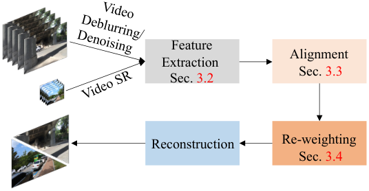
Fig. 3 shows the proposed framework. Our goal is to reconstruct a high-quality image ${\bf I}^{hq}_{0}$ from $2N+1$ consecutive low-quality images $\{{\bf I}^{lq}_{-N},\cdots,{\bf I}^{lq}_{0},\cdots,{\bf I}^{lq}_{N}\}$ . In the feature extraction module, the input frames are first downsampled with strided convolutions for video deblurring/denoising, while being processed under the same resolution for video SR. Then we utilize the proposed IAM to align input frames referring to the central frame. For simplicity, we only consider the one-side alignment in the following as the other side is processed symmetrically. Afterwards, an adaptive re-weighting module is designed to fuse the aligned features. Finally, the ${\bf I}^{hq}_{0}$ is obtained by adding the predicted residue to the original (for video deblurring/denoising) or upsampled (for video SR) input image.

3.2 Feature Extraction

As illustrated in Fig. 4, we conduct feature extraction to transform a RGB frame ${\bf I}^{lq}_{k}$ to high-dimensional feature maps ${\bf F}_{k}$ . We first utilize two convolutions with strides of 2 to downsample the feature resolutions for video deblurring and denoising (highlighted in blue dotted box in Fig. 4) for computational efficiency, while keeping the same resolution for video SR (highlighted in green dotted box in Fig. 4). Then we utilize another two convolutions with stride of 2 to obtain the pyramid representations of the input frames. At last, we fuse the pyramid features with a single convolution.

3.3 Temporal Alignment

Temporal alignment aims to align multiple neighboring features $\{{\bf F}_{-N},\cdots,{\bf F}_{-1},{\bf F}_{1},\cdots,{\bf F}_{N}\}$ to a reference ${\bf F}_{0}$ . Let $\mathcal{A}_{k}$ be the $k$ -th temporal alignment between the neighboring frame ${\bf F}_{k}$ and the reference frame ${\bf F}_{0}$ , then we have

\mathcal{A}_{k}({\bf F}_{k},{\bf F}_{0})={\hat{\bf F}}_{k}^{0},\ k\in\{-N,\cdots,-1,1,\cdots,N\},

(1)

where ${\hat{\bf F}}_{k}^{0}$ is the aligned result.

3.3.1 Progressive Alignment

In order to facilitate the long-range alignment, some recent methods chan2021basicvsr++ adopt a progressive alignment strategy. For the alignment $\mathcal{A}_{k}$ , they divide it into sequential sub-alignments $\{\mathpzc{a}_{k},\mathpzc{a}_{k-1},\cdots,\mathpzc{a}_{1}\}$ to gradually align the feature ${\bf F}_{k}$ to the reference frame ${\bf F}_{0}$ . We use $\mathpzc{a}_{i}$ to represent the sub-alginment from ${\bf F}_{i}$ to ${\bf F}_{i-1}$ :

\mathpzc{a}_{i}:{\bf F}_{i}\rightarrow{\bf F}_{i-1}.\vskip-4.0pt

(2)

As illustrated in Fig. 2(b), all neighboring frames are processed through the chained sub-alignments, indicating that the latter sub-alignments strongly depend on the former predictions. Consequently, the error incurred by an intermediate inaccurate sub-alignment will be propagated and accumulated till the end, leading to inferior performance. To alleviate the issue of error accumulation and boost the restoration quality, we propose an iterative alignment algorithm to focus on improving the accuracy of each sub-alignment $\mathpzc{a}_{i}$ .

Figure 5: PSNR differences of four SOTA video SR methods wang2019edvr; li2020mucan; chan2020basicvsr; cao2021vsrt compared to our method (dotted line) on REDS4 nah2019ntire and REDS4-Fast. The smaller the value, the larger the gap.

3.3.2 Iterative Alignment

Unlike the progressive alignment that conducts each sub-alignment only once, our algorithm iteratively refines the sub-alignments based on the previous estimation. As shown in Fig. 2(c), we start from the alignment $\mathcal{A}_{1}$ , which only contains the sub-alignment $\mathpzc{a}_{1}:{\bf F}_{1}\rightarrow{\bf F}_{0}$ , described as:

\mathcal{A}_{1}:\mathpzc{a}_{1}({\bf F}_{1},{\bf F}_{0},t=1)\Rightarrow{\hat{\bf F}}_{1}^{0},{\bf h}_{1}^{1}\,,

(3)

where ${\hat{\bf F}}_{k}^{i-1}$ refers to the aligned result of sub-alignment $\mathpzc{a}_{i}$ in $\mathcal{A}_{k}$ . And ${\bf h}^{t}_{i}$ represents the estimated motion field of the sub-alignment $\mathpzc{a}_{i}$ after being refined $t$ times.

After that, we consider the next alignment $\mathcal{A}_{2}$ by sequentially performing two sub-alignments $\{\mathpzc{a}_{2},\mathpzc{a}_{1}\}$ :

\mathcal{A}_{2}:\begin{cases}\mathpzc{a}_{2}({\bf F}_{2},{\bf F}_{1},t=1)\Rightarrow{\hat{\bf F}}_{2}^{1},{\bf h}_{2}^{1}\,,\\ \mathpzc{a}_{1}({\hat{\bf F}}_{2}^{1},{\bf F}_{0},{\bf h}^{1}_{1},t=2)\Rightarrow{\hat{\bf F}}_{2}^{0},{\bf h}_{1}^{2}\,.\\ \end{cases}

(4)

For the sub-alignment $\mathpzc{a}_{1}$ in $\mathcal{A}_{2}$ , it has already been carried out in $\mathcal{A}_{1}$ once. Thus we take the pre-estimated motion field ${\bf h}^{1}_{1}$ of $\mathpzc{a}_{1}$ in $\mathcal{A}_{1}$ as the initialization and conduct a refinement, formulated as an iterative optimization.

For the subsequent alignment $\mathcal{A}_{3}$ , two sub-alignments $\{\mathpzc{a}_{2},\mathpzc{a}_{1}\}$ will be refined as:

\mathcal{A}_{3}:\begin{cases}\mathpzc{a}_{3}({\bf F}_{3},{\bf F}_{2},t=1)\Rightarrow{\hat{\bf F}}_{3}^{2},{\bf h}_{3}^{1}\,,\\ \mathpzc{a}_{2}({\hat{\bf F}}_{3}^{2},{\bf F}_{1},{\bf h}_{2}^{1},t=2)\Rightarrow{\hat{\bf F}}_{3}^{1},{\bf h}_{2}^{2}\,,\\ \mathpzc{a}_{1}({\hat{\bf F}}_{3}^{1},{\bf F}_{0},{\bf h}_{1}^{2},t=3)\Rightarrow{\hat{\bf F}}_{3}^{0},{\bf h}_{1}^{3}\,.\\ \end{cases}

(5)

It can be concluded that, apart from the first sub-alignment $\mathpzc{a}_{k}$ in $\mathcal{A}_{k}$ , all other sub-alignments are optimized at least twice. There are two merits: ( $i$ ) The sub-alignments will be more accurate through our iterative refinements. ( $ii$ ) The sub-alignments not only rely on the pre-aligned features but also the pre-estimated motion field, making it more reliable.

To verify our claim, we evaluate our algorithm together with recent video SR models wang2019edvr; chan2020basicvsr; cao2021vsrt; li2020mucan on REDS4 nah2019ntire and REDS4-Fast ¹¹ 1 REDS4-Fast is a subset of REDS4 nah2019ntire with an average motion magnitude of 9.4 pixels, much larger than the average of REDS4 of 4.3 pixels. The optical flows are calculated by RAFT teed2020raft.. As shown in Fig. 5, our model achieves the best performance over the competing methods. Particularly, our method brings about significant improvement in the context of large motion, demonstrating the effectiveness of our IAM in the long-range alignment.

Figure 6: Illustration of our iterative sub-alignment unit for the sub-alignment

\mathpzc{a}_{i}

\mathcal{A}_{k}

{\hat{\bf F}}_{k}^{i}

is the source feature and

{\bf F}_{i-1}

is the target feature. The iterative refinement is highlighted in dashed box.

{\hat{\bf F}}_{k}^{i-1}

is the aligned result and

{\bf h}_{i}^{k+1-i}

is the refined motion field of sub-alignment

\mathpzc{a}_{i}

3.3.3 Sub-Alignment Unit

In Sec. 3.3.2, we describe the iterative alignment algorithm in detail. It is observed that for $2N$ neighboring frames, our method requires $N(N+1)$ sub-alignments. In contrast, the independent and progressive alignment schemes only need $2N$ (sub-)alignments. So it is critical to design a simple sub-alignment unit for computational efficiency. To this end, two improvements have been proposed. ( $i$ ) While the previous methods wang2019edvr; chan2020basicvsr typically adopt a pyramid alignment scheme that performs multiple-scale processing in the alignment phase, we adopt an early multi-scale fusion strategy in the feature extraction phase so that our IAM only performs single-scale alignments. ( $ii$ ) We develop a lightweight sub-alignment unit with much fewer parameters than other methods wang2019edvr; cao2021vsrt. Specifically, we use a compact structure of residual blocks to reduce computational overhead (see details in supplementary materials.).

Fig. 6 shows the structure of our sub-alignment unit. Taking the $i$ -th sub-alignment $\mathpzc{a}_{i}$ of $\mathcal{A}_{k}$ for example, we first utilize two convolutions followed by ReLU activation to estimate the initialized motion field ${\bf h}_{i}^{c}$ from the concatenation of source feature ${\hat{\bf F}}_{k}^{i}$ and target feature ${\bf F}_{i-1}$ . After that, there are two cases for the prediction ${\bf h}_{i}^{k+1-i}$ of $\mathpzc{a}_{i}$ :

{\bf h}_{i}^{k+1-i}=\begin{cases}{\bf h}_{i}^{c},&i=k\,,\\ \theta({\bf h}_{i}^{c},{\bf h}_{i}^{k-i}),&others\,.\\ \end{cases}

(6)

If $\mathpzc{a}_{i}$ is the first sub-alignment of $\mathcal{A}_{k}$ ( $i=k$ ), then no historical prediction can be reused to refine the $\mathpzc{a}_{i}$ . As a result, we simply set ${\bf h}_{i}^{c}$ as the estimated motion field of $\mathpzc{a}_{i}$ . Otherwise, we will take the last estimation ${\bf h}_{i}^{k-i}$ together with the current estimation ${\bf h}_{i}^{c}$ as input and utilize a single convolution followed by two residual blocks (dubbed as $\theta$ ) to refine the prediction. Finally, we adopt a deformable convolution dai2017deformable to adaptively sample contents from the source feature ${\hat{\bf F}}_{k}^{i}$ :

{\hat{\bf F}}_{k}^{i-1}={\rm DConv}({\hat{\bf F}}_{k}^{i},{\bf F}_{i-1},{\bf h}_{i}^{k+1-i})

(7)

Specially, if $\mathpzc{a}_{i}$ is the first sub-alignment in $\mathcal{A}^{k}$ ( $i=k$ ), Eq. 7 can be written as:

{\hat{\bf F}}_{k}^{k-1}={\rm DConv}({\bf F}_{k},{\bf F}_{k-1},{\bf h}_{k}^{1})

(8)

The sub-alignment unit is shared for all sub-alignments, largely reducing the number of learnable parameters.

3.4 Adaptive Re-weighting

Although the temporal alignment module performs motion compensation for neighboring frames, it remains vital to fuse them in an effective way. Recently, convolution-based attention mechanism becomes popular to aggregate multi-frame information liu2019image; isobe2020video; li2020learning; wu2020david. By contrast, we present a non-parametric re-weighting module to explicitly evaluate the spatially-adaptive importance of aligned frames from two perspectives. First, we evaluate the accuracy of aligned frames with respect to the reference frame. Second, we measure the consistency of aligned neighboring frames. Fig. 7 describes the pipeline of our re-weighting module.

Accuracy-Based Re-weighting.

As shown in Fig. 7(a), we measure the accuracy of aligned frames. For the reference frame ${\bf F}_{0}$ , the feature vector at position $(x,y)$ is denoted as ${\bf v}_{0}$ , i.e., ${\bf F}_{0}(x,y)={\bf v}_{0}$ . We find its corresponding $3\times 3$ patch centered at the same position in the $k$ -th aligned frame $\hat{\bf F}^{0}_{k}$ . For each feature vector on this patch, we calculate its cosine similarity (normalized inner product) with respect to ${\bf v}_{0}$ as:

{\bf S}_{k}^{x,y}(\Delta x,\Delta y)=\frac{\hat{\bf F}^{0}_{k}(x+\Delta x,y+\Delta y)}{\left\|\hat{\bf F}^{0}_{k}(x+\Delta x,y+\Delta y)\right\|_{2}}\otimes\frac{{\bf v}_{0}}{\left\|{\bf v}_{0}\right\|_{2}}\,,

(9)

where ${\bf S}_{k}^{x,y}$ is the $3\times 3$ similarity map at position $(x,y)$ and $\otimes$ represents the inner product. $(x+\Delta x,y+\Delta y)$ is the coordinate of feature vector where $\Delta x,\Delta y\in\left\{-1,0,1\right\}$ . Then a Softmax function is applied to ${\bf S}_{k}^{x,y}$ in the spatial dimension, yielding the pixel-wise weights as:

{\bf W}_{k}^{x,y}=\operatorname{Softmax}({\bf S}_{k}^{x,y})\,.

(10)

Then ${\bf W}_{k}^{x,y}$ is used to fuse feature vectors on the $3\times 3$ patch and the re-weighted result $\bar{\bf F}^{0}_{k}(x,y)$ is obtained as:

\bar{\bf F}^{0}_{k}(x,y)=\sum_{\Delta x,\Delta y}{{\bf W}_{k}^{x,y}(\Delta x,\Delta y)\odot\hat{\bf F}^{0}_{k}(x+\Delta x,y+\Delta y)}\,.

(11)

where $\odot$ denotes the Hadamard product.

Consistency-Based Re-weighting.

We first calculate the average of aligned neighboring frames yielding $\hat{\bf F}^{0}_{avg}$ , as illustrated in Fig. 7(b). For the $k$ -th aligned frame $\hat{\bf F}^{0}_{k}$ , we evaluate its consistency with other aligned frames as

{\bf C}_{k}=\operatorname{exp}({\alpha\cdot\lVert\hat{\bf F}^{0}_{k}-\hat{\bf F}^{0}_{avg}\rVert}_{2}^{2})\,,

(12)

where $\alpha$ is set to $-1$ in our experiments. It is noted that ${\bf C}_{k}$ maintains the same shape as $\hat{\bf F}^{0}_{k}$ .

Finally, we multiply the accuracy-based re-weighted feature $\bar{\bf F}^{0}_{k}$ to the consistency map ${\bf C}_{k}$ and obtain the result:

\tilde{\bf F}^{0}_{k}=\bar{\bf F}^{0}_{k}\odot{\bf C}_{k}\,.

(13)

The refined aligned feature $\tilde{\bf F}^{0}_{k}$ is passed to the reconstruction module for high-quality image regression (see Fig. 3).

4 Experiments

4.1 Implementation and Training Details

Configuration. As shown in Fig. 3, our network consists of four modules: feature extraction, alignment, re-weighting, and reconstruction. The feature extraction module in Sec. 3.2 contains 5 residual blocks for all tasks. Table 1 shows other detailed configurations, where $M$ is the number of feature channels in the network and $B$ is the number of residual blocks in the reconstruction module.

Task	Video SR	Video Deblurring	Video Denoising
Configuration	$M(128),B(40)$	$M(128),B(10)$	$M(64),B(10)$
Configuration	$M(128),B(40)$	$M(128),B(40)$	$M(64),B(10)$
GPUs	6	6	2
Patch Reso.	$64\times 64$	$128\times 128$	$128\times 128$
nFrames	5(7)	5	5
Mini-Batch	4	4	16

Table 1: The training and network configurations in different video restoration tasks.

Training. We show the training settings in Table 1. We use 2-6 NVIDIA GeForce RTX 2080 Ti GPUs to train our models for 900K iterations for all three video restoration tasks. We adopt random vertical or horizontal flipping or $90^{\circ}$ rotation for data augmentation. The initial learning rate is set to $5\times 10^{-4}$ and a cosine decay strategy is employed.

4.2 Datasets and Metrics

Video Super-Resolution. REDS nah2019ntire and Vimeo-90K xue2019video are two widely used datasets in Video SR. Vimeo-90K contains 64,612 training and 7,840 testing 7-frame sequences with resolution $448\times 256$ . The testing set is denoted as Vimeo-90K-T. In REDS, there are 266 training and 4 testing video sequences. Each sequence consists of 100 consecutive frames with resolution $1280\times 720$ . Following wang2019edvr, we denote the testing set as REDS4. Apart from these two testing datasets, we also give the quantitative results on Vid4 liu2013bayesian, which consists of 4 video clips.

Video Deblurring. We utilize the video deblurring dataset su2017deep (short for VDB) to train and evaluate our models. There are a total of 61 training and 10 testing video pairs. Each pair contains a blurry and sharp videos. The testing subset is marked as VDB-T.

Video Denoising. In this task, we aim to remove Gaussian white noises with known noise levels ( $\sigma$ ). Our model is trained on DAIVS khoreva2018video, which contains 87 training and 30 testing 540p videos. Set8 tassano2020fastdvdnet is also adopted for testing. Following tassano2020fastdvdnet, we keep a maximum of 85 frames for all training and testing sequences for a fair comparison.

Metrics. PSNR and SSIM wang2004image are used to evaluate the performance of our models in the video SR and deblurring tasks. For video denoising, following the existing methods tassano2020fastdvdnet; chen2016deep, only PSNR is reported.

Task	Video SR	Video Deblurring	Video Desnoising
Dataset	Vimeo-90K-T	VDB-T	DAVIS ( $\sigma=20$ )
Baseline	37.36	29.88	35.62
+IAM	37.72 (+0.36)	32.19 (+2.31)	36.36 (+0.74)
+IAM+ARW	37.84 (+0.48)	32.28 (+2.40)	36.73 (+1.11)

Table 2: Quantitative comparison for ablation study. PSNR (dB) is reported. “Baseline” means the model without the proposed strategies. “IAM” and “ARW” denote the iterative alignment module and adaptive re-weighting, respectively.

4.3 Analysis

In this section, we perform a comprehensive analysis of our method. We abbreviate the iterative alignment module as IAM and the adaptive re-weighting as ARW for clarity.

IAM and ARW. To evaluate the performance of the proposed IAM and ARW designs, we perform a quantitative comparison in Table 2. Starting from a baseline without these designs, we incrementally add the iterative alignment module (IAM) and adaptive re-weighting (ARW). As illustrated in Table 2, the proposed IAM brings about 0.36dB, 2.31dB and 0.74dB improvement on PSNR in the video SR, deblurring and denoising tasks, respectively. Besides, we notice that the utilization of ARW further pushes the PSNR up to a new height. Especially, it brings more improvement in the denoising task. All these results manifest the effectiveness of our proposed IAM and ARW strategies.

Methods		PSNR (dB)	SSIM	Runtime (ms)
Baseline		37.36	0.9468	153
IAM	R2	37.68 (+0.32)	0.9487	166
IAM	R3	37.72 (+0.36)	0.9490	169
ARW	Acc.	37.39 (+0.03)	0.9469	154
ARW	Con.	37.43 (+0.07)	0.9469	158
Full		37.84 (+0.48)	0.9498	170

Table 3: Ablation study on different IAM and ARW settings for video SR. The running time of each model is also reported with an input size of

7\times 112\times 64

Iterative Number in IAM. We assess the influence of iterative number in Table 3 on video SR. Compared to the baseline that performs a single prediction of each sub-alignment (identical to the progressive alignment), we gradually increase the number of refinements to 2 and 3 (denoted as R2 and R3) for sub-alignments, resulting in PSNR gains by 0.32dB and 0.36dB, respectively. It is noteworthy that the increase of running time is acceptable (13-16ms). Also, as illustrated in Fig. 8, the optical flow between the prediction and GT becomes smaller with the increase of refinements, indicating more accurate alignment. Both quantitative and qualitative results suggest that our IAM can significantly improve the alignment accuracy by reducing the error accumulation during propagation.

Re-weighting Type in ARW. As shown in Table 3, we study the proposed accuracy- and consistency-based re-weighting strategies for video SR. Compared with the baseline, the accuracy-based re-weighting leads to a 0.03dB gain while the consistency one obtains 0.07dB improvement, only costing extra 1-5ms. Fig. 9 shows some examples to illustrate the improved accuracy and consistency of our ARW. It can be observed that the model with our re-weighting module is able to restore more accurate textures while maintaining temporal consistency.

Method	REDS4 (RGB)		Vid4 (Y)
Method	$N$	PSNR/SSIM	$N$	PSNR/SSIM
Bicubic	1	26.14/0.7292	1	23.78/0.6347
TOF xue2019video	5	27.98/0.7990	7	25.89/0.7651
DUF jo2018deep	5	28.63/0.8251	7	27.33/0.8318
EDVR wang2019edvr	5	31.09/0.8800	7	27.35/0.8264
MuCAN li2020mucan	5	30.88/0.8750	7	27.26/0.8215
VSR-T cao2021vsrt	5	31.19/0.8815	7	27.36/0.8258
^∗IconVSR chan2020basicvsr	5	30.81/0.8746	7	27.39/0.8279
Ours	5	31.30/0.8850	7	27.90/0.8380

Table 4: REDS4 nah2019ntire and Vid4 liu2013bayesian results under the

\times 4

setting in video SR. The PSNR(dB)/SSIM results are evaluated under x4 setting. ’

\ast

’ indicates the results are from cao2021vsrt.

Methods	Bicubic	EDVR wang2019edvr	MuCAN li2020mucan	BasicVSR chan2020basicvsr	IconVSR chan2020basicvsr	^†BasicVSR++ chan2021basicvsr++	VSR-T cao2021vsrt	Ours
nFrame	1	1	7	7	7	7	7	7
Param.	-	20.6	19.8	6.3	8.7	7.3	43.8	17.0
RGB	29.79/0.8483	35.79/0.9374	-	-	-	-	35.88/0.9380	35.96/0.9389
Y	31.32/0.8684	37.61/0.9489	37.32/0.9465	37.18/0.9450	37.47/0.9476	37.79/0.9500	37.71/0.9494	37.84/0.9498

Table 5: Vimeo-90K-T xue2019video results in video SR. The PSNR(dB)/SSIM results are obtained under the

\times 4

setting. Numbers in red and blue refer to the best and second-best results. ’

{\dagger}

’ means BasicVSR++ uses an additional REDS dataset for pretraining.

Dataset	$\sigma$	VNLB arias2018video	V-BM4D maggioni2012video	VNLnet chen2016deep	FastDVD tassano2020fastdvdnet	Ours
Set8	10	37.26	36.05	37.10	36.44	37.25
	20	33.72	32.19	33.88	33.43	34.05
	30	31.74	30.00	-	31.68	32.19
	40	30.39	28.48	30.55	30.46	30.89
	50	29.24	27.33	29.47	29.53	29.90
DAVIS	10	38.85	37.58	35.83	38.71	39.75
	20	35.68	33.88	34.49	35.77	36.73
	30	33.73	31.65	-	34.04	34.89
	40	32.32	30.05	32.32	32.82	33.56
	50	31.13	28.80	31.43	31.86	32.51

Table 6: Set8 tassano2020fastdvdnet and DAVIS khoreva2018video results in video denoising. PSNR(dB) results are reported.

4.4 Comparison with State-of-The-Art Methods

We compare our method with state-of-the-art approaches quantitatively and qualitatively in the video SR, video deblurring and video denoising tasks.

Video Super-resolution. Table 5 and Table 9 exhibit the quantitative results of our method and existing video SR methods xue2019video; jo2018deep; wang2019edvr; li2020mucan; chan2020basicvsr; haris2019recurrent; cao2021vsrt; chan2021basicvsr++ on Vimeo-90K-T xue2019video, REDS4 nah2019ntire and Vid4 liu2013bayesian datasets. Compared to the representative independent wang2019edvr and progressive chan2020basicvsr alignment methods, our method obtains superior Y-channel PSNR performance with 0.23dB and 0.66dB improvement on Vimeo-90K-T, respectively. In addition, our model also surpasses the VSR-T cao2021vsrt by 0.13dB, which has much more parameters. While BasicVSR++ chan2021basicvsr++ uses an additional dataset for pretraining, our results are still the best. In terms of the Vid4 liu2013bayesian dataset, our method achieves significant improvement with 0.51dB on PSNR compared with IconVSR chan2020basicvsr. Besides, Fig. 10 shows the visual comparison on Vimeo-90K-T and REDS4. Our model recovers much clearer text and more accurate structures compared to other methods.

Video Denoising. Following previous methods tassano2020fastdvdnet; arias2018video; chen2016deep, we adopt Set8 tassano2020fastdvdnet and DAVIS khoreva2018video as our benchmarks in the video denoising task. The quantitative results are reported in Table 6. Our model achieves the best results under most noise levels. Especially, compared with the second-best approaches, our method largely improves the PSNR by 0.37dB and 0.65dB under the noise level $\sigma=50$ on Set8 and DAVIS, respectively. Fig. 11 presents some qualitative results. It is observed that our method restores richer and clearer textures compared with other approaches.

Video Deblurring. We compare our method with several recent video deblurring approaches hyun2017online; su2017deep; wang2019edvr; zhou2019spatio; pan2020cascaded on VDB-T su2017deep. As illustrated in Table 1, two models with different sizes (10 or 40 residual blocks) are developed, denoted as “Ours-M” and “Ours”. From Table 7, compared to the second best ARVo pan2020cascaded, we see that our model achieves 0.12dB and 0.013 improvement on PSNR and SSIM, respectively. Some visual examples illustrated in Fig. 12 also demonstrate that our model is able to handle soame challenging cases with complex motion blur.

Meth.	EDVR wang2019edvr	STFA zhou2019spatio	Pan pan2020cascaded	ARVo li2021arvo	Ours-M	Ours
Param.	23.6M	5.4M	16.2M	-	12.7M	16.7M
PSNR	28.51	31.24	32.13	32.80	32.28	32.92
SSIM	0.864	0.934	0.927	0.935	0.942	0.948

Table 7: VDB-T su2017deep results in video deblurring. “Ours-M” and “Ours” denote our medium and standard models.

4.5 Limitation

In this work, the proposed designs are mainly for improving the accuracy of the long-range alignment. There remains plenty of room to optimize the modeling of subtle motion. Besides, further improving the efficiency of the alignment pipeline is also our future target.

5 Conclusion

In this paper, we propose a simple yet effective iterative alignment algorithm (IAM) and an efficient adaptive reweighting strategy (ARW) to better utilize multi-frame information. The quantitative and qualitative results of three video restoration tasks illustrate the effectiveness of our method. Besides, we show that our method is general to be deployed in existing video processing systems to further improve their performance. We will explore more video-based tasks in the future. The code will be publicly available to promote the development of the community.

References

(1) Pablo Arias and Jean-Michel Morel. Video denoising via empirical bayesian estimation of space-time patches. Journal of Mathematical Imaging and Vision, 60(1):70–93, 2018.
(2) Jiezhang Cao, Yawei Li, Kai Zhang, and Luc Van Gool. Video super-resolution transformer. arXiv, 2021.
(3) Kelvin CK Chan, Xintao Wang, Ke Yu, Chao Dong, and Chen Change Loy. Basicvsr: The search for essential components in video super-resolution and beyond. arXiv preprint arXiv:2012.02181, 2020.
(4) Kelvin CK Chan, Shangchen Zhou, Xiangyu Xu, and Chen Change Loy. Basicvsr++: Improving video super-resolution with enhanced propagation and alignment. arXiv preprint arXiv:2104.13371, 2021.
(5) Xinyuan Chen, Li Song, and Xiaokang Yang. Deep rnns for video denoising. In Applications of Digital Image Processing XXXIX, volume 9971, page 99711T. International Society for Optics and Photonics, 2016.
(6) Jifeng Dai, Haozhi Qi, Yuwen Xiong, Yi Li, Guodong Zhang, Han Hu, and Yichen Wei. Deformable convolutional networks. In Proceedings of the IEEE international conference on computer vision, pages 764–773, 2017.
(7) Muhammad Haris, Gregory Shakhnarovich, and Norimichi Ukita. Recurrent back-projection network for video super-resolution. In Proceedings of the IEEE Conference on Computer Vision and Pattern Recognition, pages 3897–3906, 2019.
(8) Tae Hyun Kim, Kyoung Mu Lee, Bernhard Scholkopf, and Michael Hirsch. Online video deblurring via dynamic temporal blending network. In CVPR, pages 4038–4047, 2017.
(9) Takashi Isobe, Xu Jia, Shuhang Gu, Songjiang Li, Shengjin Wang, and Qi Tian. Video super-resolution with recurrent structure-detail network. In European Conference on Computer Vision, pages 645–660. Springer, 2020.
(10) Younghyun Jo, Seoung Wug Oh, Jaeyeon Kang, and Seon Joo Kim. Deep video super-resolution network using dynamic upsampling filters without explicit motion compensation. In CVPR, pages 3224–3232, 2018.
(11) Anna Khoreva, Anna Rohrbach, and Bernt Schiele. Video object segmentation with language referring expressions. In Asian Conference on Computer Vision, pages 123–141. Springer, 2018.
(12) Dongxu Li, Chenchen Xu, Kaihao Zhang, Xin Yu, Yiran Zhong, Wenqi Ren, Hanna Suominen, and Hongdong Li. Arvo: Learning all-range volumetric correspondence for video deblurring. In Proceedings of the IEEE/CVF Conference on Computer Vision and Pattern Recognition, pages 7721–7731, 2021.
(13) Feng Li, Huihui Bai, and Yao Zhao. Learning a deep dual attention network for video super-resolution. IEEE Transactions on Image Processing, 29:4474–4488, 2020.
(14) Wenbo Li, Xin Tao, Taian Guo, Lu Qi, Jiangbo Lu, and Jiaya Jia. Mucan: Multi-correspondence aggregation network for video super-resolution. In ECCV, pages 335–351. Springer, 2020.
(15) Wenbo Li, Kun Zhou, Lu Qi, Nianjuan Jiang, Jiangbo Lu, and Jiaya Jia. Lapar: Linearly-assembled pixel-adaptive regression network for single image super-resolution and beyond. 33, 2020.
(16) Ce Liu and Deqing Sun. On bayesian adaptive video super resolution. IEEE transactions on pattern analysis and machine intelligence, 36(2):346–360, 2013.
(17) Ding Liu, Zhaowen Wang, Yuchen Fan, Xianming Liu, Zhangyang Wang, Shiyu Chang, and Thomas Huang. Robust video super-resolution with learned temporal dynamics. In Proceedings of the IEEE International Conference on Computer Vision, pages 2507–2515, 2017.
(18) Zhi-Song Liu, Li-Wen Wang, Chu-Tak Li, Wan-Chi Siu, and Yui-Lam Chan. Image super-resolution via attention based back projection networks. In 2019 IEEE/CVF International Conference on Computer Vision Workshop (ICCVW), pages 3517–3525. IEEE, 2019.
(19) Matteo Maggioni, Giacomo Boracchi, Alessandro Foi, and Karen Egiazarian. Video denoising, deblocking, and enhancement through separable 4-d nonlocal spatiotemporal transforms. IEEE Transactions on image processing, 21(9):3952–3966, 2012.
(20) Seungjun Nah, Sungyong Baik, Seokil Hong, Gyeongsik Moon, Sanghyun Son, Radu Timofte, and Kyoung Mu Lee. Ntire 2019 challenge on video deblurring and super-resolution: Dataset and study. In Proceedings of the IEEE/CVF Conference on Computer Vision and Pattern Recognition Workshops, pages 0–0, 2019.
(21) Jinshan Pan, Haoran Bai, and Jinhui Tang. Cascaded deep video deblurring using temporal sharpness prior. In Proceedings of the IEEE/CVF Conference on Computer Vision and Pattern Recognition, pages 3043–3051, 2020.
(22) Anurag Ranjan and Michael J Black. Optical flow estimation using a spatial pyramid network. In Proceedings of the IEEE conference on computer vision and pattern recognition, pages 4161–4170, 2017.
(23) Yaniv Romano, John Isidoro, and Peyman Milanfar. Raisr: rapid and accurate image super resolution. IEEE Transactions on Computational Imaging, 3(1):110–125, 2016.
(24) Shuochen Su, Mauricio Delbracio, Jue Wang, Guillermo Sapiro, Wolfgang Heidrich, and Oliver Wang. Deep video deblurring for hand-held cameras. In CVPR, pages 1279–1288, 2017.
(25) Matias Tassano, Julie Delon, and Thomas Veit. Fastdvdnet: Towards real-time deep video denoising without flow estimation. In CVPR, pages 1354–1363, 2020.
(26) Zachary Teed and Jia Deng. Raft: Recurrent all-pairs field transforms for optical flow. In European conference on computer vision, pages 402–419. Springer, 2020.
(27) Yapeng Tian, Yulun Zhang, Yun Fu, and Chenliang Xu. Tdan: Temporally-deformable alignment network for video super-resolution. In Proceedings of the IEEE/CVF Conference on Computer Vision and Pattern Recognition, pages 3360–3369, 2020.
(28) Xintao Wang, Kelvin CK Chan, Ke Yu, Chao Dong, and Chen Change Loy. Edvr: Video restoration with enhanced deformable convolutional networks. In Proceedings of the IEEE Conference on Computer Vision and Pattern Recognition Workshops, pages 0–0, 2019.
(29) Zhou Wang, Alan C Bovik, Hamid R Sheikh, and Eero P Simoncelli. Image quality assessment: from error visibility to structural similarity. IEEE transactions on image processing, 13(4):600–612, 2004.
(30) Bartlomiej Wronski, Ignacio Garcia-Dorado, Manfred Ernst, Damien Kelly, Michael Krainin, Chia-Kai Liang, Marc Levoy, and Peyman Milanfar. Handheld multi-frame super-resolution. ACM Transactions on Graphics (TOG), 38(4):1–18, 2019.
(31) Junru Wu, Xiang Yu, Ding Liu, Manmohan Chandraker, and Zhangyang Wang. David: Dual-attentional video deblurring. In Proceedings of the IEEE/CVF Winter Conference on Applications of Computer Vision, pages 2376–2385, 2020.
(32) Xiangyu Xu, Muchen Li, and Wenxiu Sun. Learning deformable kernels for image and video denoising. arXiv preprint arXiv:1904.06903, 2019.
(33) Tianfan Xue, Baian Chen, Jiajun Wu, Donglai Wei, and William T Freeman. Video enhancement with task-oriented flow. IJCV, 127(8):1106–1125, 2019.
(34) Peng Yi, Zhongyuan Wang, Kui Jiang, Junjun Jiang, and Jiayi Ma. Progressive fusion video super-resolution network via exploiting non-local spatio-temporal correlations. In Proceedings of the IEEE/CVF International Conference on Computer Vision, pages 3106–3115, 2019.
(35) Yulun Zhang, Kunpeng Li, Kai Li, Lichen Wang, Bineng Zhong, and Yun Fu. Image super-resolution using very deep residual channel attention networks. In ECCV, pages 286–301, 2018.
(36) Ruofan Zhou and Sabine Susstrunk. Kernel modeling super-resolution on real low-resolution images. In ICCV, pages 2433–2443, 2019.
(37) Shangchen Zhou, Jiawei Zhang, Jinshan Pan, Haozhe Xie, Wangmeng Zuo, and Jimmy Ren. Spatio-temporal filter adaptive network for video deblurring. In ICCV, pages 2482–2491, 2019.

Appendix A Residual Block

As illustrated in Table 8, our residual block is comprised of two convolutions, where the first convolution is followed by ReLU activation. In previous works wang2019edvr; chan2020basicvsr; cao2021vsrt, the channel numbers typically keep identical within the residual block. In contrast, we set the channel dimension of hidden representations ( $M_{1}$ ) no more than 64 to reduce the parameters of our network and speed up the training and inference phases:

M_{1}=max(M//2,64),

(14)

Input	x
Layer1	Conv( $M$ , $M_{1}$ ,3,1) + ReLU
Layer2	Conv( $M_{1}$ , $M$ ,3,1) $\Rightarrow y$
Output	x+y

Table 8: The structure of our residual block.

M

refers to the channel number of input.

Appendix B More Reuslts

B.1 Temporal Consistency

We compare the temporal consistency of our method with several state-of-art video SR approaches jo2018deep; wang2019edvr; li2020mucan; chan2020basicvsr. The visual results are illustrated in Figure 13. It is observed that other methods fail to restore the consistent textures clearly. While our method empowered with iterative alignment and two adaptively reweighting strategies is able to generate realistic image contents that are closest to the ground-truth.

Methods	nFrame	Clip_000	Clip_011	Clip_015	Clip_020	Average
Bicubic	1	24.55/0.6489	26.06/0.7261	28.52/0.8034	25.41/0.7386	26.14/0.7292
RCAN zhang2018image	1	26.17/0.7371	29.34/0.8255	31.85/0.8881	27.74/0.8293	28.78/0.8200
TOF xue2019video	7	26.52/0.7540	27.80/0.7858	30.67/0.8609	26.92/0.7953	27.98/0.7990
DUF jo2018deep	7	27.30/0.7937	28.38/0.8056	31.55/0.8846	27.30/0.8164	28.63/0.8251
EDVR wang2019edvr	5	28.01/0.8250	32.17/0.8864	34.06/0.9206	30.09/0.8881	31.09/0.8800
MuCAN li2020mucan	5	27.99/0.8219	31.84/0.8801	33.90/0.9170	29.78/0.8811	30.88/0.8750
^∗BasicVSR chan2020basicvsr	5	27.67/0.8114	31.27/0.8740	33.58/0.9135	29.71/0.8803	30.56/0.8698
^∗IconVSR chan2020basicvsr	5	27.83/0.8182	31.69/0.8798	33.81/0.9164	29.90/0.8841	30.81/0.8746
VSR-T cao2021vsrt	5	28.06/0.8267	32.28/0.8883	34.15/0.9199	30.26/0.8912	31.19/0.8815
Ours	5	28.16/0.8316	32.24/0.8889	34.53/0.9275	30.26/0.8920	31.30/0.8850

Table 9: Quantitative comparison on REDS4 nah2019ntire benchmark under

\times 4

setting for video super-resolution. Numbers in red and blue refer to the best and second-best results. All the results are evaluated in the RGB channel. ’

\ast

’ indicates the results are from cao2021vsrt.

Clip Name	Bicubic	DUF jo2018deep	EDVR wang2019edvr	MuCAN li2020mucan	BasicVSR chan2020basicvsr	IconVSR chan2020basicvsr	VSR-T cao2021vsrt	Ours
Calendar (Y)	20.39/0.5720	24.04/0.8110	24.05/0.8147	-	-	-	24.08/0.8125	24.65/0.8270
City (Y)	25.16/0.6028	28.27/0.8313	28.00/0.8122	-	-	-	27.94/0.8107	29.92/0.8428
Foliage (Y)	23.47/0.5666	26.41/0.7709	26.34/0.7635	-	-	-	26.33/0.7635	26.41/0.7652
Walk (Y)	26.10/0.7974	30.60/0.9141	31.02/0.9152	-	-	-	31.10/0.9163	31.15/0.9167
Average (Y)	23.78/0.6347	27.33/0.8318	27.35/0.8264	27.26/0.8215	27.24/0.8251	27.39/0.8279	27.36/0.8258	27.90/0.8380
Average (RGB)	22.37/0.6098	25.79/0.8136	25.83/0.8077	-	-	-	-	26.57/0.8235

Table 10: Quantitative comparison on Vid4 liu2013bayesian under x4 setting for video super-resolution. We report the PSNR (dB)/SSIM results on both the RGB and the Y channel. Numbers in red and blue refer to the best and second-best results.

B.2 Comparison with State-of-the-art

In Table 9 and 10, we give the detialed comparison with several state-of-the-art video SR approaches wang2019edvr; chan2020basicvsr; cao2021vsrt; cao2021vsrt on REDS4 nah2019ntire and Vid4 liu2013bayesian. The PSNR and SSIM of each video sequence are reported. For most video clips of both two validation sets, our model consistently achieves the best performance. Moreover, we provide extensive qualitative comparison on UDM10 yi2019progressive, Vid4 liu2013bayesian, Vimeo-90K-T xue2019video, and REDS4 nah2019ntire for video SR (in Figure 14, 15), VDB-T su2017deep for video deblurring (in Figure 16) and Set8 tassano2020fastdvdnet, DAIVS khoreva2018video for video denoising (in Figure 17). All the qualitative results demonstrate that our method has the capacity to handle various challenging cases in these three video restoration tasks.

B.3 Video Results

We also provide three videos for visual inspection. “city.mp4”. This video illustrates the visual comparison between bicubic and our method on a Vid4 clip for video super-resolution. It can be observed that our method restores much clear image details (e.g., the finer structure of buildings).
“IMG0030.mp4”. This video demonstrates the visual results of our method on a testing sequence of VDB-T su2017deep for the video deblurring task. The burry input and the generated frames are shown in it.
“motorbike.mp4”. This video shows the restoration results on a sequence of Set8 tassano2020fastdvdnet for video denoising.