An Analysis of the Numerical Stability of the Immersed Boundary Method

We consider a cubic domain $\mathbf{\Omega}=[0,L]\times[0,L]\times[0,L]$ with periodic boundary conditions and the domain of material coordinates $\mathbf{s}=(s_{1},s_{2})$ is $\mathbf{S}=[0,L]\times[0,L]$. The material coordinates $(s_{1},s_{2})$ are introduced to describe the position of the immersed boundary and its target position. Here, let $(x,y,z)$ be the Cartesian coordinates and let the boundary be a plane parallel to the xy-plane and located at $z=\sigma_{3}\in[0,L]$. Ideally, we want the immersed boundary to be no-slip and therefore the immersed boundary is expected to be fixed at its initial position, which we call the target position here. Thus, the target position, denoted here by $\mathbf{X}^{0}$, in the Cartesian coordinates is given by $\mathbf{X}^{0}(s_{1},s_{2})=\mathbf{X}(s_{1},s_{2},0)=(s_{1}+\sigma_{1},s_{2}+\sigma_{2},\sigma_{3})$, where $\mathbf{X}(s_{1},s_{2},t)$ is the boundary position and $t$ is the time. Note that the immersed boundary $\mathbf{X}(s_{1},s_{2},t)$ is assumed to move with the fluid near it by the formulation of the immersed boundary method and we cannot strictly fix it at its target position $\mathbf{X}^{0}(s_{1},s_{2})$. Therefore, the immersed boundary $\mathbf{X}(s_{1},s_{2},t)$ may change its position over time and it depends on time $t$. Equation (5), which we will introduce later in this section, describes how we exert a spring-like feedback force on the immersed boundary $\mathbf{X}(s_{1},s_{2},t)$ in order to keep it near its initial positions $\mathbf{X}^{0}(s_{1},s_{2})$.

The equations of motion are

$$\rho\frac{\partial\mathbf{u}}{\partial t}+\nabla\mathbf{p}=\mu\Delta\mathbf{u}+\mathbf{f}$$

(1)

$$\nabla\cdot\mathbf{u}=0$$

(2)

$$\mathbf{f}(\mathbf{x},t)=\int_{\mathbf{S}}\mathbf{F}(s_{1},s_{2},t)\delta(\mathbf{x}-\mathbf{X}^{0}(s_{1},s_{2}))ds_{1}ds_{2}$$

(3)

$$\frac{\partial\mathbf{X}}{\partial t}(s_{1},s_{2},t)=\int_{\mathbb{R}^{3}}\mathbf{u}(\mathbf{x},t)\delta(\mathbf{x}-\mathbf{X}^{0}(s_{1},s_{2}))d\mathbf{x}$$

(4)

$$\mathbf{F}(s_{1},s_{2},t)=-K(\mathbf{X}(s_{1},s_{2},t)-\mathbf{X}^{0}(s_{1},s_{2}))$$

(5)

Equations (1) and (2) are the time-dependent incompressible Stokes equations, which are the linearized incompressible Navier-Stokes equations with the nonlinear convective term being dropped. Equations (3) and (4) are interaction equations which translate between Eulerian and Lagrangian variables. Equation (3) describes the body force $\mathbf{f}(\mathbf{x},t)$ that is applied to the fluid and equation (4) describes the evaluation of the fluid velocity at the immersed boundary. As mentioned above, equation (5) describes the force generated by the stiff springs that hold the immersed boundary $\mathbf{X}(s_{1},s_{2},t)$ in place.

Since the velocity evaluated at the boundary in (4) should be zero because of the no-slip boundary condition, $\mathbf{X}(s_{1},s_{2},t)-\mathbf{X}^{0}(s_{1},s_{2})$ is the integral over time of the error that has been made in enforcing the no-slip condition. That is why our formula for $\mathbf{F}(s_{1},s_{2},t)$ in equation (5) can be interpreted as a feedback mechanism (specifically, an integral controller) for enforcing the no-slip condition.

The fluid domain is discretized by an $N\times N\times N$ grid with a uniform mesh width $h=L/N$. Let $Z_{N}=\{0,1,\cdots,N-1\}$ and $Z_{NP}=\{0,1,\cdots,NP-1\}$ be sets of integer indices, where $P\in\mathbb{N}$. Then, the fluid grid is defined by $\mathbf{\Omega}_{h}=\{\mathbf{j}h:\mathbf{j}=(j_{1},j_{2},j_{3})\in Z_{N}^{3}\}$ and the grid points are $\mathbf{x}_{\mathbf{j}}=(j_{1}h,j_{2}h,j_{3}h)$. Let the boundary grid be defined by $\mathbf{S}_{h_{B}}=\{\mathbf{k}h_{B}+\bm{\sigma}:\mathbf{k}=(k_{1},k_{2})\in Z_{NP}^{2}\}$, where $h_{B}=L/(NP)$ is the mesh width of the boundary grid and $\bm{\sigma}=(\mathbf{\sigma}_{1},\mathbf{\sigma}_{2},\mathbf{\sigma}_{3})$ is a three-dimensional shift of the immersed boundary. Note that the boundary grid plane is defined such that it is parallel to the xy-plane and its z-coordinate, namely $\sigma_{3}$, is general. In other words, the boundary plane does not have to lie on one of the fluid grid planes. The target position of the discretized immersed boundary is thus given by $\mathbf{X}^{0}_{k_{1},k_{2}}=\mathbf{X}^{0}(k_{1}h_{B},k_{2}h_{B})=(k_{1}h_{B}+\mathbf{\sigma}_{1},k_{2}h_{B}+\mathbf{\sigma}_{2},\mathbf{\sigma}_{3})$ and the discretized boundary itself is given by $\mathbf{X}_{k_{1},k_{2}}(t)=\mathbf{X}(k_{1}h_{B},k_{2}h_{B},t)$. Similarly, the force at the boundary $\mathbf{F}_{k_{1},k_{2}}(t)$ is defined by $\mathbf{F}_{k_{1},k_{2}}(t)=\mathbf{F}(k_{1}h_{B},k_{2}h_{B},t)$. In the above definitions, we use subscripts to indicate indices $(k_{1},k_{2})\in Z_{NP}^{2}$. The spatial discretization of equation (1) - (5) is then as follows

$$\rho\frac{\partial\mathbf{u}}{\partial t}+\nabla_{h}\mathbf{p}=\mu\Delta_{h}\mathbf{u}+\mathbf{f}$$

(6)

$$\nabla_{h}\cdot\mathbf{u}=0$$

(7)

$$\mathbf{f}(\mathbf{x}_{\mathbf{j}},t)=\sum_{\mathbf{k}\in Z_{NP}^{2}}\mathbf{F}_{k_{1},k_{2}}(t)\delta_{h}(\mathbf{x}_{\mathbf{j}}-\mathbf{X}^{0}_{k_{1},k_{2}})h_{B}^{2}$$

(8)

$$\frac{\partial\mathbf{X}_{k_{1},k_{2}}}{\partial t}(t)=\sum_{\mathbf{j}\in Z_{N}^{3}}\mathbf{u}(\mathbf{x}_{\mathbf{j}},t)\delta_{h}(\mathbf{x}_{\mathbf{j}}-\mathbf{X}^{0}_{k_{1},k_{2}})h^{3}$$

(9)

$$\mathbf{F}_{k_{1},k_{2}}(t)=-K(\mathbf{X}_{k_{1},k_{2}}(t)-\mathbf{X}^{0}_{k_{1},k_{2}})$$

(10)

Note that the smoothed Dirac delta function $\delta_{h}$ is evaluated at target positions $\mathbf{X}^{0}_{k_{1},k_{2}}$ instead of $\mathbf{X}_{k_{1},k_{2}}(t)$. For a sufficiently large $K$, we expect $\mathbf{X}_{k_{1},k_{2}}(t)$ to be approximately equal to $\mathbf{X}^{0}_{k_{1},k_{2}}$, and by using $\mathbf{X}^{0}_{k_{1},k_{2}}$, we linearizes the boundary condition. The difference operators $\nabla_{h}$ and $\Delta_{h}$ are defined as follows:

$$(\nabla_{h}p)_{\alpha}(\mathbf{x}_{\mathbf{j}})=\frac{p(\mathbf{x}_{\mathbf{j}}+h\mathbf{e}_{\alpha})-p(\mathbf{x}_{\mathbf{j}}-h\mathbf{e}_{\alpha})}{2h},\quad\alpha=1,2,3$$

(11)

$$(\nabla_{h}\cdot\mathbf{u})(\mathbf{x}_{\mathbf{j}})=\sum_{\alpha=1}^{3}\frac{\mathbf{u}(\mathbf{x}_{\mathbf{j}}+h\mathbf{e}_{\alpha})-\mathbf{u}(\mathbf{x}_{\mathbf{j}}-h\mathbf{e}_{\alpha})}{2h}$$

(12)

$$(\Delta_{h}\mathbf{u})(\mathbf{x}_{\mathbf{j}})=\sum_{\alpha=1}^{3}\frac{\mathbf{u}(\mathbf{x}_{\mathbf{j}}+h\mathbf{e}_{\alpha})+\mathbf{u}(\mathbf{x}_{\mathbf{j}}-h\mathbf{e}_{\alpha})-2\mathbf{u}(\mathbf{x}_{\mathbf{j}})}{h^{2}}$$

(13)

In the above definitions, $\{\mathbf{e}_{1},\mathbf{e}_{2},\mathbf{e}_{3}\}$ is the standard basis of $\mathbb{R}^{3}$ and $\mathbf{j}\in Z_{N}^{3}$, so ${\bf x}_{\mathbf{j}}\in\Omega_{h}$.

We can eliminate $\mathbf{X}_{k_{1},k_{2}}(t)$ from our system by differentiating (10) with respect to $t$ and it follows that

$$\frac{\partial\mathbf{F}_{k_{1},k_{2}}}{\partial t}(t)=-K\sum_{\mathbf{j}\in Z_{N}^{3}}\mathbf{u}(\mathbf{x}_{\mathbf{j}},t)\delta(\mathbf{x}_{\mathbf{j}}-\mathbf{X}^{0}_{k_{1},k_{2}})h^{3}$$

(14)

Note that $\mathbf{F}(k_{1},k_{2},t)$ is then proportional to the accumulated error up to time t that has occurred in enforcing the no-slip condition at the location $\mathbf{X}^{0}(k_{1},k_{2})$. In the above equations, the smoothed Dirac delta function $\delta_{h}$ is the standard IB 4-point delta function defined [11] by

$$\delta_{h}(\mathbf{x}_{\mathbf{j}})=\frac{1}{h^{3}}\phi(j_{1})\phi(j_{2})\phi(j_{3})$$

(15)

where

$$\phi(r)=\begin{cases}\frac{3-2|r|+\sqrt{1+4|r|-4r^{2}}}{8},\quad|r|\leq 1\\ \frac{5-2|r|-\sqrt{-7+12|r|-4r^{2}}}{8},\quad|r|\in[1,2]\\ 0,\quad|r|>2\end{cases}$$

(16)

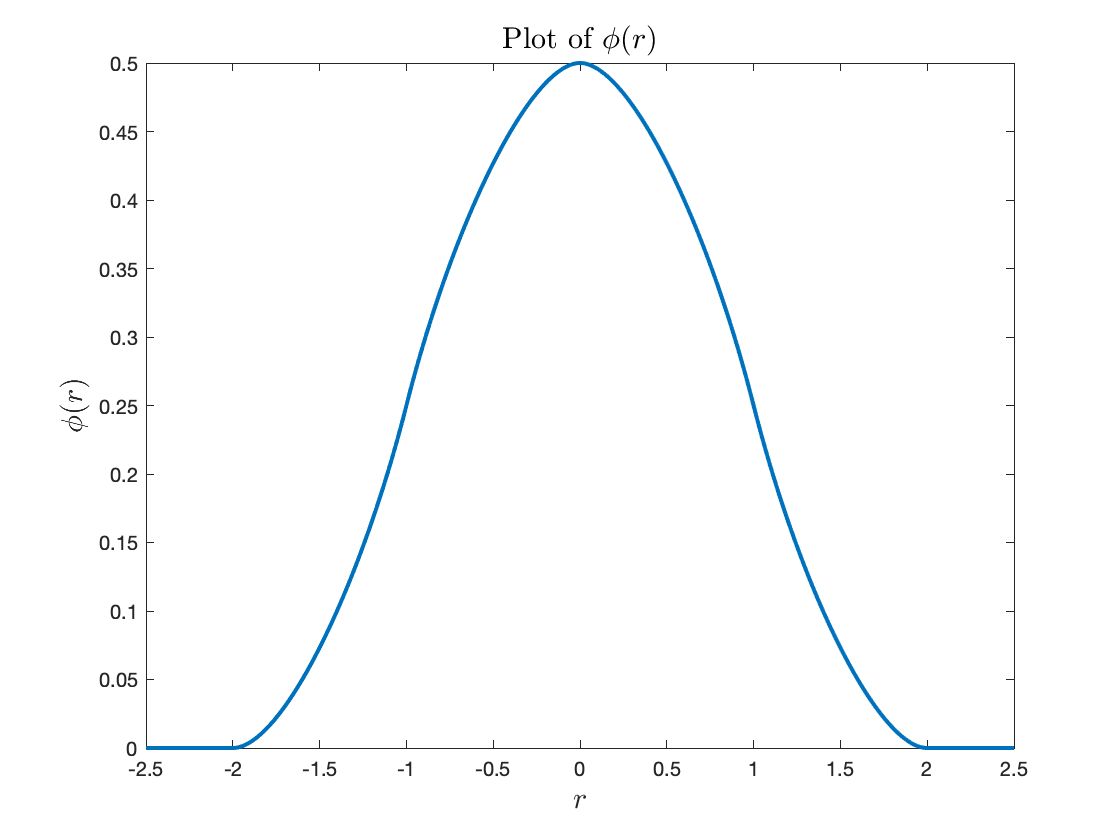
Let $\bm{\epsilon}=\bm{\sigma}/h$, so that $\bm{\epsilon}$ is the shift vector in units of meshwidth of the fluid grid. Then, equation (8) and (14) can be rewritten as follows

$$\mathbf{f}(\mathbf{x}_{\mathbf{j}},t)=\sum_{\mathbf{k}\in Z_{NP}^{2}}\mathbf{F}_{k_{1},k_{2}}(t)\phi(j_{1}-\frac{k_{1}}{P}-\epsilon_{1})\phi(j_{2}-\frac{k_{2}}{P}-\epsilon_{2})\phi(j_{3}-\epsilon_{3})\frac{h_{B}^{2}}{h^{3}}$$

(17)

$$\frac{\partial\mathbf{F}_{k_{1},k_{2}}}{\partial t}(t)=-K\sum_{\mathbf{j}\in Z_{N}^{3}}\mathbf{u}(\mathbf{x}_{\mathbf{j}},t)\phi(j_{1}-\frac{k_{1}}{P}-\epsilon_{1})\phi(j_{2}-\frac{k_{2}}{P}-\epsilon_{2})\phi(j_{3}-\epsilon_{3})$$

(18)

For discretization in time, we first write down a second-order Runge-Kutta scheme as in [11], but this scheme will turn out to be equivalent to a simple leapfrog scheme because we have here dropped the nonlinear convective term of the Navier-Stokes equations and also because the centering of the smoothed Dirac delta function $\delta_{h}$ at fixed positions.

In writing this scheme, it is helpful to introduce the following notation

$$\mathbf{U}_{k_{1},k_{2}}(t)=\sum_{\mathbf{j}\in Z_{N}^{3}}\mathbf{u}(\mathbf{x}_{\mathbf{j}},t)\phi(j_{1}-\frac{k_{1}}{P}-\epsilon_{1})\phi(j_{2}-\frac{k_{2}}{P}-\epsilon_{2})\phi(j_{3}-\epsilon_{3})$$

(19)

From now on, we use superscripts to indicate the time step. The Runge-Kutta scheme is then as follows

$$\mathbf{F}^{n+\frac{1}{2}}_{k_{1},k_{2}}=\mathbf{F}^{n}_{k_{1},k_{2}}-\frac{\Delta t}{2}K\mathbf{U}^{n}_{k_{1},k_{2}}$$

(20)

$$\mathbf{f}^{n+\frac{1}{2}}({\bf x}_{\mathbf{j}})=\sum_{\mathbf{k}\in Z_{NP}^{2}}\mathbf{F}^{n+\frac{1}{2}}_{k_{1},k_{2}}\phi(j_{1}-\frac{k_{1}}{P}-\epsilon_{1})\phi(j_{2}-\frac{k_{2}}{P}-\epsilon_{2})\phi(j_{3}-\epsilon_{3})\frac{h_{B}^{2}}{h^{3}}$$

(21)

$$\begin{cases}\rho\frac{\mathbf{u}^{n+\frac{1}{2}}-\mathbf{u}^{n}}{{\Delta t}/2}+\nabla_{h}\tilde{\mathbf{p}}^{n+\frac{1}{2}}=\mu\Delta_{h}\mathbf{u}^{n+\frac{1}{2}}+\mathbf{f}^{n+\frac{1}{2}}\\ \nabla_{h}\cdot\mathbf{u}^{n+\frac{1}{2}}=0\end{cases}$$

(22)

$$\begin{cases}\rho\frac{\mathbf{u}^{n+1}-\mathbf{u}^{n}}{{\Delta t}}+\nabla_{h}\mathbf{p}^{n+\frac{1}{2}}=\mu\Delta_{h}\frac{\mathbf{u}^{n+1}+\mathbf{u}^{n}}{2}+\mathbf{f}^{n+\frac{1}{2}}\\ \nabla_{h}\cdot\mathbf{u}^{n+1}=0\end{cases}$$

(23)

$$\mathbf{F}^{n+1}_{k_{1},k_{2}}=\mathbf{F}^{n}_{k_{1},k_{2}}-{\Delta t}K\mathbf{U}^{n+\frac{1}{2}}_{k_{1},k_{2}}$$

(24)

To see how this scheme simplifies, we notice that systems of equations (22) and (23), which have the same source term, are independent of each other, since $\mathbf{u}^{n+\frac{1}{2}}$ does not appear in (23) as it would if we were considering the Naiver-Stokes equations. Moreover, if we have the solution of (23), then we also have the solution of (22) simply by setting

$$\begin{cases}\mathbf{u}^{n+\frac{1}{2}}=\frac{\mathbf{u}^{n}+\mathbf{u}^{n+1}}{2}\\ \tilde{\mathbf{p}}^{n+\frac{1}{2}}=\mathbf{p}^{n+\frac{1}{2}}\end{cases}$$

(25)

Equation (25) implies that

$$\mathbf{U}^{n+\frac{1}{2}}=\frac{\mathbf{U}^{n}+\mathbf{U}^{n+1}}{2}$$

(26)

But note that it does so only because of the use of delta functions centered at fixed locations. Thus, we can dispense with (22), and also we can rewrite (24) as

$$\mathbf{F}^{n+1}_{k_{1},k_{2}}=\mathbf{F}^{n+\frac{1}{2}}_{k_{1},k_{2}}-\frac{{\Delta t}}{2}K\mathbf{U}^{n+1}_{k_{1},k_{2}}$$

(27)

Lowering n by 1 gives

$$\mathbf{F}^{n}_{k_{1},k_{2}}=\mathbf{F}^{n-\frac{1}{2}}_{k_{1},k_{2}}-\frac{{\Delta t}}{2}K\mathbf{U}^{n}_{k_{1},k_{2}}$$

(28)

and substitution of this into (20) gives

$$\mathbf{F}^{n+\frac{1}{2}}_{k_{1},k_{2}}=\mathbf{F}^{n-\frac{1}{2}}_{k_{1},k_{2}}-{\Delta t}K\mathbf{U}^{n}_{k_{1},k_{2}}$$

(29)

Therefore, we are left with a leapfrog scheme that can be written as follows:

$$\mathbf{F}^{n+\frac{1}{2}}_{k_{1},k_{2}}=\mathbf{F}^{n-\frac{1}{2}}_{k_{1},k_{2}}-{\Delta t}K\mathbf{U}^{n}_{k_{1},k_{2}}$$

(30)

$$\mathbf{f}^{n+\frac{1}{2}}({\bf x}_{\mathbf{j}})=\sum_{\mathbf{k}\in Z_{NP}^{2}}\mathbf{F}^{n+\frac{1}{2}}_{k_{1},k_{2}}\phi(j_{1}-\frac{k_{1}}{P}-\epsilon_{1})\phi(j_{2}-\frac{k_{2}}{P}-\epsilon_{2})\phi(j_{3}-\epsilon_{3})\frac{h_{B}^{2}}{h^{3}}$$

(31)

$$\begin{cases}\rho\frac{\mathbf{u}^{n+1}-\mathbf{u}^{n}}{{\Delta t}}+\nabla_{h}\mathbf{p}^{n+\frac{1}{2}}=\mu\Delta_{h}\frac{\mathbf{u}^{n+1}+\mathbf{u}^{n}}{2}+\mathbf{f}^{n+\frac{1}{2}}\\ \nabla_{h}\cdot\mathbf{u}^{n+1}=0\end{cases}$$

(32)

To analyze the numerical stability of the above leapfrog scheme, we introduce the discrete Fourier transform defined on the fluid grid by

$$\widehat{\mathbf{u}}(\mathbf{\bm{\xi}})=\sum_{\mathbf{j}\in Z_{N}^{3}}e^{-i\frac{2\pi}{N}\mathbf{j}\cdot\mathbf{\bm{\xi}}}\mathbf{u}(\mathbf{x}_{\mathbf{j}})$$

(33)

$$\mathbf{u}(\mathbf{x}_{\mathbf{j}})=\frac{1}{N^{3}}\sum_{\mathbf{\bm{\xi}}\in Z_{N}^{3}}e^{i\frac{2\pi}{N}\mathbf{j}\cdot\mathbf{\bm{\xi}}}\widehat{\mathbf{u}}(\mathbf{\bm{\xi}})$$

(34)

Similarly, we define the discrete Fourier transform on the boundary grid as follows

$$\widetilde{\mathbf{F}}(m_{1},m_{2})=\sum_{(k_{1},k_{2})\in Z_{NP}^{2}}e^{-i\frac{2\pi}{NP}(k_{1}m_{1}+k_{2}m_{2})}\mathbf{F}_{k_{1},k_{2}}$$

(35)

$$\mathbf{F}_{k_{1},k_{2}}=\frac{1}{N^{2}P^{2}}\sum_{(m_{1},m_{2})\in Z_{NP}^{2}}e^{i\frac{2\pi}{NP}(k_{1}m_{1}+k_{2}m_{2})}\widetilde{\mathbf{F}}(m_{1},m_{2})$$

(36)

The difference operators $\nabla_{h}$ and $\Delta_{h}$ become multiplication operators in Fourier space

$$(\widehat{\nabla}_{h})_{\alpha}(\bm{\xi})=\frac{i}{h}\sin(\frac{2\pi}{N}\xi_{\alpha}),\quad\alpha=1,2,3$$

(37)

$$(\widehat{\Delta}_{h})(\bm{\xi})=-\frac{4}{h^{2}}\sum_{\alpha=1}^{3}\sin^{2}(\frac{\pi}{N}\xi_{\alpha})$$

(38)

The following definition of the Fourier series representation of the function $\phi$ will turn out to be useful:

$$\phi(r)=\sum_{q=-\infty}^{\infty}\Phi(q)e^{i\frac{2\pi}{N}qr}$$

(39)

$$\Phi(q)=\frac{1}{N}\int_{-\frac{N}{2}}^{\frac{N}{2}}\phi(r)e^{-i\frac{2\pi}{N}qr}dr=\frac{1}{N}\int_{-2}^{2}\phi(r)e^{-i\frac{2\pi}{N}qr}dr$$

(40)

Here, we reinterpret the IB 4-point delta function $\phi(r)$ as a Fourier series with period $N$, since $r$ is in units of meshwidth of the fluid grid, and in those units our periodic domain has length $N$ in each coordinate direction. Since the IB 4-point delta function has support $[-2,2]$, we should here assume that $N\geq 4$ to make the periodic extension possible. By using equation (39) to rewrite equation (19) with $t=n\Delta t$ in terms of $\Phi$, and by using the evenness of the function $\phi$, we get the following:

$$\mathbf{U}^{n}_{k_{1},k_{2}}=\sum_{q_{1},q_{2},q_{3}=-\infty}^{\infty}\Phi(q_{1})\Phi(q_{2})\Phi(q_{3})e^{i\frac{2\pi}{NP}(k_{1}q_{1}+k_{2}q_{2})}e^{i\frac{2\pi}{N}(\mathbf{q}\cdot\bm{\epsilon})}\widehat{\mathbf{u}}^{n}(\mathbf{q})$$

(41)

Now we multiply both sides of (41) by $e^{-i\frac{2\pi}{NP}(k_{1}m_{1}+k_{2}m_{2})}$ and sum over $(k_{1},k_{2})\in Z_{NP}^{2}$. To evaluate this sum, we make use of

$$\sum_{k\in Z_{NP}}e^{i\frac{2\pi}{NP}k(q-m)}=\begin{cases}NP,\hskip 5.0pt\text{if}\hskip 5.0ptq-m\hskip 5.0pt\text{is an integer multiple of}\hskip 5.0ptNP\\ 0,\hskip 5.0pt\text{otherwise}\end{cases}$$

(42)

In this way, we get the result

	$\displaystyle\widetilde{\mathbf{U}}^{n}(m_{1},m_{2})=$	$\displaystyle(NP)^{2}e^{i\frac{2\pi}{N}(m_{1}\epsilon_{1}+m_{2}\epsilon_{2})}(\sum_{l_{1}=-\infty}^{\infty}\Phi(m_{1}+l_{1}NP)e^{i2\pi Pl_{1}\epsilon_{1}})$
		$\displaystyle(\sum_{l_{2}=-\infty}^{\infty}\Phi(m_{2}+l_{2}NP)e^{i2\pi Pl_{2}\epsilon_{2}})(\sum_{q_{3}=-\infty}^{\infty}\Phi(q_{3})e^{i\frac{2\pi}{N}q_{3}\epsilon_{3}}\widehat{\mathbf{u}}^{n}(m_{1},m_{2},q_{3}))$		(43)

Similarly, we make use of (39) on the right-hand side of (31) , apply the definition (35), multiply both sides of the equation by $e^{-i\frac{2\pi}{N}(\bm{\xi}\cdot\mathbf{j})}$, and sum over $\mathbf{j}\in Z_{N}^{3}$, we get the result

		$\displaystyle\widehat{\mathbf{f}}^{n+\frac{1}{2}}(\bm{\xi})=\frac{h_{B}^{2}N^{3}}{h^{3}}e^{-i\frac{2\pi}{N}(\bm{\xi}\cdot\bm{\epsilon})}\left(\sum_{l_{3}=-\infty}^{\infty}\Phi(\xi_{3}+l_{3}N)e^{-i2\pi l_{3}\epsilon_{3}}\right)$
		$\displaystyle\left(\sum_{l_{1},l_{2}=-\infty}^{\infty}\Phi(\xi_{1}+l_{1}N)\Phi(\xi_{2}+l_{2}N)e^{-i2\pi(l_{1}\epsilon_{1}+l_{2}\epsilon_{2})}\widetilde{F}^{n+\frac{1}{2}}(\xi_{1}+l_{1}N,\xi_{2}+l_{2}N)\right)$		(44)

Here we have used

$$\sum_{k\in Z_{N}}e^{i\frac{2\pi}{N}k(q-\xi)}=\begin{cases}N,\hskip 5.0pt\text{if}\hskip 5.0ptq-\xi\hskip 5.0pt\text{is an integer multiple of}\hskip 5.0ptN\\ 0,\hskip 5.0pt\text{otherwise}\end{cases}$$

(45)

In equation (41), we can use the periodicity of $\widehat{\mathbf{u}}^{n}$ to rewrite the last factor as follows:

$$\left(\sum_{m_{3}\in Z_{N}}(\sum_{l_{3}=-\infty}^{\infty}\Phi(m_{3}+l_{3}N)e^{i2\pi l_{3}\epsilon_{3}})e^{i\frac{2\pi}{N}m_{3}\epsilon_{3}}\widehat{\mathbf{u}}^{n}(\mathbf{m})\right)$$

(46)

where we let

$$q_{3}=m_{3}+l_{3}N$$

(47)

In a similar way, we can use the periodicity of $\widetilde{\mathbf{F}}$ to rewrite the sum over $(l_{1},l_{2})$ in equation (2.3). Note that $\widetilde{\mathbf{F}}$ is periodic in each of its arguments with period $NP$. Let

$$l_{1}=p_{1}+Pl_{1}^{{}^{\prime}}$$

(48)

$$l_{2}=p_{2}+Pl_{2}^{{}^{\prime}}$$

(49)

Then, the sum over $(l_{1},l_{2})$ in equation (2.3) can be rewritten as follows

	$\displaystyle\sum_{(p_{1},p_{2})\in Z_{P}^{2}}$	$\displaystyle\left(\sum_{l_{1}=-\infty}^{\infty}\Phi(\xi_{1}+NP_{1}+NPl_{1}^{{}^{\prime}})e^{-i2\pi Pl_{1}^{{}^{\prime}}\epsilon_{1}}\right)$
		$\displaystyle\left(\sum_{l_{2}=-\infty}^{\infty}\Phi(\xi_{2}+NP_{2}+NPl_{2}^{{}^{\prime}})e^{-i2\pi Pl_{2}^{{}^{\prime}}\epsilon_{2}}\right)$
		$\displaystyle e^{-2\pi(p_{1}\epsilon_{1}+p_{2}\epsilon_{2})\widetilde{\mathbf{F}}^{n+\frac{1}{2}}(\xi_{1}+Np_{1},\xi_{2}+Np_{2})}$		(50)

To simplify the notation, we let

$$a(m,\epsilon)=\sum_{l=-\infty}^{\infty}\Phi(m+lNP)e^{i2\pi Pl\epsilon}$$

(51)

$$b(\xi,\epsilon)=\sum_{l=-\infty}^{\infty}\Phi(\xi+lN)e^{i2\pi l\epsilon}$$

(52)

Since $\phi$ is real and even, $\Phi$ is real and even, we also have

$$\overline{a(m,\epsilon)}=\sum_{l=-\infty}^{\infty}\Phi(m+lNP)e^{-i2\pi Pl\epsilon}$$

(53)

$$\overline{b(\xi,\epsilon)}=\sum_{l=-\infty}^{\infty}\Phi(\xi+lN)e^{-i2\pi l\epsilon}$$

(54)

Moreover, we let

	$\displaystyle\widehat{\mathbf{F}}^{n+\frac{1}{2}}(\xi_{1},\xi_{2},\epsilon_{2},\epsilon_{2})=\sum_{(p_{1},p_{2})\in Z_{P}^{2}}$	$\displaystyle\overline{a(\xi_{1}+Np_{1},\epsilon_{1})}\hskip 3.0pt\overline{a(\xi_{2}+Np_{2},\epsilon_{2})}$
		$\displaystyle e^{-i2\pi(p_{1}\epsilon_{1}+p_{2}\epsilon_{2})}\widetilde{\mathbf{F}}^{n+\frac{1}{2}}(\xi_{1}+Np_{1},\xi_{2}+Np_{2})$		(55)

Therefore, equation (41) and equation (2.3) become

	$\displaystyle\widetilde{\mathbf{U}}^{n}(\xi_{1}+Np_{1},\xi_{2}+Np_{2})=$	$\displaystyle(NP)^{2}a(\xi_{1}+Np_{1},\epsilon_{1})a(\xi_{2}+Np_{2},\epsilon_{2})$
		$\displaystyle\left(\sum_{\xi_{3}\in Z_{N}}b(\xi_{3},\epsilon_{3})e^{i\frac{2\pi}{N}(\bm{\epsilon}\cdot\bm{\xi})}e^{i2\pi(p_{1}\epsilon_{1}+p_{2}\epsilon_{2})}\widehat{\mathbf{u}}^{n}(\bm{\xi})\right)$		(56)

$$\widehat{\mathbf{f}}^{n+\frac{1}{2}}(\bm{\xi})=\frac{h_{B}^{2}N^{3}}{h^{3}}e^{-i\frac{2\pi}{N}(\bm{\xi}\cdot\bm{\epsilon})}\widehat{\mathbf{F}}^{n+\frac{1}{2}}(\xi_{1},\xi_{2},\epsilon_{2},\epsilon_{2})\overline{b(\xi_{3},\epsilon_{3})}$$

(57)

By equation (30), we also have

$$\widetilde{\mathbf{F}}^{n+\frac{1}{2}}(\xi_{1}+Np_{1},\xi_{2}+Np_{2})=\widetilde{\mathbf{F}}^{n-\frac{1}{2}}(\xi_{1}+Np_{1},\xi_{2}+Np_{2})-\Delta tK\widetilde{\mathbf{U}}^{n}(\xi_{1}+Np_{1},\xi_{2}+Np_{2})$$

(58)

After application of the discrete Fourier transform defined on the fluid grid, the system (32) becomes

$$\begin{cases}\rho\frac{\widehat{\mathbf{u}}^{n+1}-\widehat{\mathbf{u}}^{n}}{{\Delta t}}+\widehat{\nabla}_{h}\widehat{\mathbf{p}}^{n+\frac{1}{2}}=\mu\widehat{\Delta}_{h}\frac{\widehat{\mathbf{u}}^{n+1}+\widehat{\mathbf{u}}^{n}}{2}+\widehat{\mathbf{f}}^{n+\frac{1}{2}}\\ \widehat{\nabla}_{h}\cdot\widehat{\mathbf{u}}^{n+1}=0\end{cases}$$

(59)

We can eliminate the pressure term $\widehat{\mathbf{p}}^{n+\frac{1}{2}}$ and solve for $\widehat{\mathbf{u}}^{n+1}$ by introducing a $3\times 3$ matrix

$$\widehat{P}(\mathbf{\bm{\xi}})=I-\frac{\left(\widehat{\nabla}_{h}(\mathbf{\bm{\xi}})\right)\left(\widehat{\nabla}_{h}(\mathbf{\bm{\xi}})\right)^{\ast}}{\left(\widehat{\nabla}_{h}(\mathbf{\bm{\xi}})\right)^{\ast}\left(\widehat{\nabla}_{h}(\mathbf{\bm{\xi}})\right)}$$

(60)

where $\ast$ denotes the Hermitian conjugate of a matrix and I is the $3\times 3$ identity matrix. The projection matrix $\widehat{P}(\mathbf{\bm{\xi}})$ projects a vector field $\widehat{\mathbf{u}}^{n+1}$ onto its divergence-free component by the Helmholtz decomposition. Therefore, $\widehat{P}(\mathbf{\bm{\xi}})\widehat{\nabla}_{h}\widehat{\mathbf{p}}^{n+\frac{1}{2}}=0$ and $\widehat{P}(\mathbf{\bm{\xi}})\widehat{\mathbf{u}}^{n+1}=\widehat{\mathbf{u}}^{n+1}$. Then the system (60) is reduced to

$$\rho\frac{\widehat{\mathbf{u}}^{n+1}-\widehat{\mathbf{u}}^{n}}{{\Delta t}}=\mu\widehat{\Delta}_{h}\frac{\widehat{\mathbf{u}}^{n+1}+\widehat{\mathbf{u}}^{n}}{2}+\widehat{P}(\mathbf{\bm{\xi}})\widehat{\mathbf{f}}^{n+\frac{1}{2}}\\$$

(61)

Solving for $\widehat{\mathbf{u}}^{n+1}$ gives

$$\widehat{\mathbf{u}}^{n+1}(\bm{\xi})=\frac{\left(1+\frac{{\Delta t}\mu}{2\rho}\widehat{\Delta}_{h}(\bm{\xi})\right)\widehat{\mathbf{u}}^{n}(\bm{\xi})+\frac{\rho}{{\Delta t}}\widehat{P}(\mathbf{\bm{\xi}})\widehat{\mathbf{f}}^{n+\frac{1}{2}}}{1-\frac{{\Delta t}\mu}{2\rho}\widehat{\Delta}_{h}(\bm{\xi})}$$

(62)

To study the stability of the leapfrog scheme, we look for a solution in which all the variables are multiplied by a possibly complex number $z$ at each time step. The type of the solution that we seek is defined by

$$\widehat{\mathbf{u}}^{n}(\bm{\xi})=z^{n}\widehat{\mathbf{u}}^{0}(\bm{\xi})$$

(63)

$$\widetilde{\mathbf{F}}^{n+\frac{1}{2}}(m_{1},m_{2})=z^{n}\widetilde{\mathbf{F}}^{\frac{1}{2}}(m_{1},m_{2})$$

(64)

$$\widehat{\mathbf{f}}^{n+\frac{1}{2}}(\bm{\xi})=z^{n}\widehat{\mathbf{f}}^{\frac{1}{2}}(\bm{\xi})$$

(65)

Here the superscript on $z$ is actually a power, whereas all of other superscripts are merely labels indicating time steps. Then, after substituting (63-65) into the Fourier transform of the leapfrog scheme, we obtain the following system:

	$\displaystyle\widehat{\mathbf{F}}^{\frac{1}{2}}(\xi_{1},\xi_{2},\epsilon_{2},\epsilon_{2})=\sum_{(p_{1},p_{2})\in Z_{P}^{2}}$	$\displaystyle\overline{a(\xi_{1}+Np_{1},\epsilon_{1})}\hskip 3.0pt\overline{a(\xi_{2}+Np_{2},\epsilon_{2})}$
		$\displaystyle e^{-i2\pi(p_{1}\epsilon_{1}+p_{2}\epsilon_{2})}\widetilde{\mathbf{F}}^{\frac{1}{2}}(\xi_{1}+Np_{1},\xi_{2}+Np_{2})$		(66)

$$\widetilde{\mathbf{F}}^{\frac{1}{2}}(\xi_{1}+Np_{1},\xi_{2}+Np_{2})=\frac{-z}{z-1}\Delta tK\widetilde{\mathbf{U}}^{0}(\xi_{1}+Np_{1},\xi_{2}+Np_{2})$$

(67)

	$\displaystyle\widetilde{\mathbf{U}}^{0}(\xi_{1}+Np_{1},\xi_{2}+Np_{2})=$	$\displaystyle(NP)^{2}a(\xi_{1}+Np_{1},\epsilon_{1})a(\xi_{2}+Np_{2},\epsilon_{2})$
		$\displaystyle e^{i2\pi(p_{1}\epsilon_{1}+p_{2}\epsilon_{2})}\left(\sum_{\xi_{3}\in Z_{N}}b(\xi_{3},\epsilon_{3})e^{i\frac{2\pi}{N}(\bm{\epsilon}\cdot\bm{\xi})}\widehat{\mathbf{u}}^{0}(\bm{\xi})\right)$		(68)

$$\widehat{\mathbf{u}}^{0}(\bm{\xi})=\frac{\frac{{\Delta t}}{\rho}\widehat{P}(\mathbf{\bm{\xi}})\widehat{\mathbf{f}}^{\frac{1}{2}}(\bm{\xi})}{(z-1)-(z+1)\frac{{\Delta t}\mu}{2\rho}\widehat{\Delta}_{h}(\bm{\xi})}$$

(69)

References

- [1] D. Boffi, L. Gastaldi, and L. Heltai, Numerical stability of the finite element immersed boundary method, Mathematical Models and Methods in Applied Sciences, 17 (2007), pp. 1479–1505.
- [2] L. Heltai, On the stability of the finite element immersed boundary method, Computers & Structures, 86 (2008), pp. 598–617.
- [3] Y. Kim and C. S. Peskin, Penalty immersed boundary method for an elastic boundary with mass, Physics of Fluids, 19 (2007), p. 053103.
- [4] Y. Kim and C. S. Peskin, A penalty immersed boundary method for a rigid body in fluid, Physics of Fluids, 28 (2016), p. 033603.
- [5] F.-H. Lin and J. Tong, Solvability of the Stokes immersed boundary problem in two dimensions, Communications on Pure and Applied Mathematics, 72 (2019), pp. 159–226.
- [6] Y. Liu and Y. Mori, Properties of discrete delta functions and local convergence of the immersed boundary method, SIAM J. Numer. Anal., 50 (2012), pp. 2986–3015.
- [7] Y. Liu and Y. Mori, convergence of the immersed boundary method for stationary Stokes problems, SIAM Journal on Numerical Analysis, 52 (2014), pp. 496–514.
- [8] Y. Mori, Convergence proof of the velocity field for a Stokes flow immersed boundary method, Communications on Pure and Applied Mathematics, 61 (2008), pp. 1213–1263.
- [9] Y. Mori, A. Rodenberg, and D. Spirn, Well-posedness and global behavior of the Peskin problem of an immersed elastic filament in Stokes flow, Communications on Pure and Applied Mathematics, 72 (2019), pp. 887–980.
- [10] C. S. Peskin, Flow patterns around heart valves: A numerical method, Journal of Computational Physics, 10 (1972), pp. 252–271.
- [11] C. S. Peskin, The immersed boundary method, Acta Numerica, 11 (2002), p. 479–517.
- [12] J. M. Stockie and B. R. Wetton, Analysis of stiffness in the immersed boundary method and implications for time-stepping schemes, Journal of Computational Physics, 154 (1999), pp. 41–64.
- [13] J. M. Stockie and B. T. R. Wetton, Stability analysis for the immersed fiber problem, SIAM Journal on Applied Mathematics, 55 (1995), pp. 1577–1591.
- [14] J. J. Stoker, Water Waves: The Mathematical Theory with Applications, John Wiley & Sons, Ltd, 1992.