A Fast Non-parametric Approach for Local Causal Structure Learning
Abstract
We study the problem of causal structure learning with essentially no assumptions on the functional relationships and noise. We develop DAG-FOCI, a computationally fast algorithm for this setting that is based on the FOCI variable selection algorithm in [1]. DAG-FOCI outputs the set of parents of a response variable of interest. We provide theoretical guarantees of our procedure when the underlying graph does not contain any (undirected) cycle containing the response variable of interest. Furthermore, in the absence of this assumption, we give a conservative guarantee against false positive causal claims when the set of parents is identifiable. We demonstrate the applicability of DAG-FOCI on simulated as well as a real dataset from computational biology [28].
Keywords: Causal inference, Graphical models, Markov boundary, Nonlinear models, Structural equation models.
1 Introduction
Causal reasoning is important in many areas, including the sciences, decision making, and public policy. The gold standard method for determining causal relations uses randomized control experiments, but the cost and ethical concerns often hinder their feasibility. Hence, it is worth estimating causal relations from observational data, that is, data obtained from observing a system without any interventions. We study this problem in a non-parametric setting where we assume that all relevant variables are observed, excluding latent variables.
This paper proposes a computationally efficient algorithm for local causal structure learning around a target variable of interest without restricting the functional forms, error distributions, or relying on conditional independence testing. The price to be paid for this generality is in terms of conservativeness. We provide finite sample guarantees that our algorithm will not wrongly claim a causal edge when the target variable has multiple parents: it may not lead to many causal findings, but when the underlying causal graph is a polytree, the parental set is correctly identified. From a practical perspective, in an observational study without latent variables, this is so far the only causal inference algorithm that does not rely on conditional independence testing and protects against false causal claims when there are multiple causes, in very general non-parametric models.
To develop our methodology, we consider a setting where the variables satisfy the Causal Markov property with respect to a directed acyclic graph (DAG) and are generated according to a structural equation model (SEM). As announced above, no assumptions or restrictions are imposed on the functional forms or the error distributions. We focus on recovering the set of parents of a given target variable (maybe multiple since the Markov equivalence class can entail more than one set of parents). Estimating the entire DAG can be viewed as combining the local neighborhood structures of all the nodes [24, 40].
Our proposed algorithm, dubbed DAG-FOCI, consists of two stages. In the first stage, we identify the local structure in terms of the Markov boundary of the target variable. This is done using a greedy algorithm named FOCI, introduced in [1]. FOCI does not rely on any statistical testing or distributional assumptions. Furthermore, it does not require the specification of any tuning parameters and is computationally efficient. In the second stage of DAG-FOCI, we combine some pairwise independence tests with the output of the first stage (for several targets) to determine the multi-set of parents of the target variable. We emphasize here that the second stage requires only marginal statistical testing, a much easier and better-posed task than conditional independence testing. Our theoretical guarantees for DAG-FOCI require a condition dubbed ‘-Markov Gap’, which states that the target variable has larger dependencies with members of its Markov boundary than with variables outside of its Markov boundary. The -Markov Gap condition is crucial for ensuring that the greedy algorithm in the first stage of DAG-FOCI is successful. Under such an assumption, we establish a finite sample guarantee that no false-positive causal edges are claimed by DAG-FOCI when the target variable of interest has more than one parent. Furthermore, again for finite sample cases and when the target variable has multiple parents, we show that DAG-FOCI identifies the parental set if the underlying DAG is a polytree.
The outline of this paper is as follows. In Section 2, we present our algorithm DAG-FOCI. We explain our main theoretical results in Section 3. In Section 4, we describe how to incorporate interventional data into DAG-FOCI for additional identifiability. Applications to simulated and real data are presented in Section 5. We conclude with future directions in Section 6.
1.1 Related Work
Prior work on causal structure learning can be broadly categorized into two groups: score-based algorithms and constraint-based approaches using conditional independence testing. The latter focuses mostly on Gaussian distributions [14, 17, 5] and transformable to Gaussian distributions [11]; one can also strengthen these approaches by using a kernel-based tests for conditional independence [7]. Score-based methods have been worked out for the Gaussian case [4, 36, 16], and there is a substantial amount of work when putting additional restrictions on the functional forms (e.g. nonlinear but additive errors [12, 27, 3, 21]), or on the error distributions (e.g. non-Gaussian and additive error [31] or equal error noise variances [25]). Some methods also combine score-based and constraint-based approaches [35, 20].
As highlighted above, in contrast to DAG-FOCI, both constraint-based and score-based methods rely on techniques or assumptions which are challenging or restrictive in the purely non-parametric case. In particular, constraint-based methods such as the PC and IC algorithms [32, 23] require conditional independence testing, which is known to be a hard problem in non-parametric settings [30]. Although there has been a large body of research exploring different ideas for conditional independence testing, there is no model-free and non-parametric method with theoretical guarantees for this purpose: one has to restrict the model class to obtain power against arbitrary alternatives. Hence, many constraint-based methods are vulnerable in applications where the data may not satisfy the properties needed for the validity of the conditional independence test. Similarly, non-parametric score-based methods are not tractable in general. In addition to requiring distributional assumptions, score-based methods can become computationally infeasible in high-dimensional settings. Improving the speed of score-based methods involves either using ad-hoc optimization [2, 41] or requiring tree structure or additive noise model [13].
The authors in [10, 9] propose polynomial-time algorithms for structural learning in non-parametric settings, and provide finite-sample theoretical guarantees for their methods. However, their methodology and theoretical analysis require more stringent assumptions than the ones imposed in this paper. Specifically, [10] places an ‘equal variance’ type condition on the error distributions and [9] requires non-source nodes to have higher conditional entropy compared to at least one of their ancestors.11 1 In general, this assumption is not satisfied: consider the simple example and where and is a measurable function. Furthermore, neither method provides false discovery control guarantees when their assumptions are violated.
1.2 Notations and Definitions
We represent a DAG with a node set and a collection of directed edges . We denote a directed edge by or . In this case, is a parent of , and is a child of . If there is a directed path , then is a descendent of , and is an ancestor of . The skeleton of is the undirected graph obtained from by substituting directed edges with undirected edges. Nodes , , and form a v-structure in a DAG if and there is no edge between and . In this case, and are spouses and node is called an unshielded collider. More generally, if and can have an edge connecting them, node is called a collider.
For the joint probability distribution on , the Causal Markov property holds if every variable is independent of its non-descendants conditional on its parents. The Markov equivalence class of is the set of all DAGs that encode the same set of conditional independencies. Two DAGs are Markov equivalent if and only if they have the same skeleton and the same v-structures [38]. Let be the Markov equivalence class of DAG . We denote the set of parents, children, and spouses of in DAG respectively by , , and . For simplicity in the notation and and for a special DAG of interest , we drop the subscripts, e.g, etc. We represent the collection of all parental sets in the Markov equivalence class by . Note that may be less than as DAGs and in the Markov equivalence class may encode the same set of parents for , i.e. . Note that if is a source node in , then . From the distribution of observational data, one can in general only identify the Markov equivalence class; in particular, this is the case in the fully non-parametric setting which we consider in this work.
For any , is the random vector consisting of all ’s excluding . For an index set , the random vector of corresponding features is denoted by . For , is a Markov blanket or a sufficient set for if and only if . A minimal Markov blanket is called a Markov boundary, i.e., a Markov blanket is a Markov boundary if no strict subset of it is a Markov blanket. In this paper, we always assume that the Markov boundary is unique; indeed this is the case under mild assumptions [22, Th.4.3]. We denote the unique Markov boundary of by . It is well-known that for any , .
Finally, our methodological development and theoretical analysis is motivated by the graphical notions of tree-neighborhood and polytree, which are defined below:
Definition 1.1.
Node satisfies a tree-neighborhood property if any cycle in the skeleton of contains at most one member of .
Definition 1.2.
A polytree is a DAG whose skeleton is a tree.
2 Our algorithm DAG-FOCI
We consider the random vector and denote by a response variable of special interest. We posit that the underlying distribution of satisfies the Causal Markov property with respect to a DAG and is parameterized by the following structural equation model (SEM):
| (1) |
Here, is a measurable function, and are jointly independent noise variables from non-degenerate probability laws.
We always assume that the observed data consists of independent and identically distributed realizations from the SEM in (1). Extensions to interventional data are presented in Section 4.
As described in the introduction, our algorithm DAG-FOCI consists of two stages. In the first stage, we deploy the non-parametric variable selection procedure FOCI [1] to obtain the local Markov structure around the node : the Markov boundary of , denoted as , as well as the Markov blanket of each of the variables in . In the second stage, we combine the local Markov structures around to identify the parents of . The description of DAG-FOCI is presented in Algorithm 1.
In Sections 2.1 and 2.2, we explain Algorithm 1 in more details. In Section 2.1 we explain how the Markov boundary search is done using FOCI and in Section 2.2 we elaborate on steps 2-3.
2.1 Stage I of DAG-FOCI: Finding the Markov Boundary
For Markov boundary estimation in step 1 of Algorithm 1, we use the model-free variable selection algorithm FOCI [1]. FOCI is based on the non-parametric and distribution-free measure of dependence CODEC [1]. For a random variable and random vectors and where and , CODEC quantifies the dependency of on conditional on as
| (2) |
where is the probability law of . When or in other words does not have any components, which measures the dependency of on without any conditioning.
Based on samples, the following estimator for was introduced in [1]:
| (3) |
Here, is the rank of among all the other ’s, is the index of the nearest neighbor of among other ’s, and is the index of the nearest neighbor of among the rest of ’s. The nearest neighbors are measured with respect to a metric of choice; in this paper, we use the euclidean distance. Since the estimator (3) only relies on the ranks and the nearest neighbor indices, it is computationally efficient and estimated with computational complexity . For the target variable , and features , FOCI proceeds in the following forward step-wise manner: In each step, FOCI selects one of the remaining variables until none of them adds any “predictive power”. Let be the set of selected variables by FOCI up to and including step , initializing with . In step , FOCI selects , if the maximum value is positive. Otherwise FOCI stops and returns . Note that FOCI possesses a natural stopping rule and does not require the user to specify any stopping criterion. We present a summary of FOCI in Algorithm 2.
In [1, Th.6.1], the authors show that under mild assumptions, and for large enough sample size , is with high probability a Markov blanket for . In general, there is no bound on the size of this Markov blanket, and it may not be the minimal one. In Theorem 3.1 we show that under a so-called -Markov Gap assumption (A.3), the estimated Markov blanket by FOCI is minimal and hence is the Markov boundary.
2.2 Stage II of DAG-FOCI: Combining Markov boundaries to identify parents
We next describe steps 2 and 3 of Algorithm 1, namely: how DAG-FOCI combines the information of Markov blankets obtained from the first stage to estimate the set(s) of parents. To develop these steps, we assume that the tree-neighborhood assumption for node is satisfied (see Definition 1.1); nonetheless, we will show in Theorem 3.5 that as long as is a collider, DAG-FOCI will not output wrong causal conclusions even when the tree-neighborhood assumption does not hold.
Let be the collection of all sets of parents of in the Markov equivalence class of (as defined in Section 1.2). The logic behind steps 2 and 3 heavily relies on the following properties, satisfied for every parental set :
- (p1)
If , then for all :
- (p2)
If , then for all
- (p3)
For , , , and iff there exists such that
- (p4)
If , we have and if , we have for all
To better understand step 2, we characterize the population analogue of , denoted by . The set is the output of step 2 if the Markov boundary search and pairwise independence tests of DAG-FOCI are performed without making any errors. Appealing to properties (p1)-(p4), we conclude that contains all possible sets of parents, i.e. . Furthermore, contains only nodes that are connected to in the skeleton of , i.e. for every . Thus, in population, step 2 removes all spouses from the Markov boundary of without excluding any parental nodes.
We propose the following procedure to obtain efficiently. Starting from an empty graph with the vertex set , we form an undirected graph as follows: for every pair of nodes , edge is added to if and . Properties (p1) and (p2) guarantee that consists of disjoint fully connected subgraphs, i.e. such that ’s are complete graphs and . Among these connected components, we let be those that contain pairwise independent nodes. Algorithm 3 presents the finite-sample analogue to obtain the estimate .
Thus far, we have presented an efficient approach to combine local Markov structure with pairwise independence tests to arrive at a superset of the true parental set . We now describe step 3, which removes non-parental elements of when possible. To that end, we highlight the following relation where satisfies:
- (e1)
for all
- (e2)
for all
Properties (e1) and (e2) are implied by (p1)-(p4) and motivate step 3 of Algorithm 1. Specifically, according to property (e1), the set consists of non-parental elements and should ideally be removed from . Property (e2) guides how we remove (when possible) in step 3.
Specifically, consider all the possible scenarios for the set : there exists a single set with , there exists multiple sets with , and for all . Appealing to properties (e1)-(e2) and (p4) , scenario implies that and scenario leads to a contradiction. These observations explain the following logic in step 3 of Algorithm 1: if contains exactly one set such that , we let ; if there are multiple sets with , DAG-FOCI returns an error message. Finally, in scenario , we cannot distinguish from , as property (p4) states that can consist of all singletons. This observation explains the following logic in step 3 of Algorithm 1: if for all , we let .
We remark that scenario highlights a fundamental challenge with applying a local algorithm, like DAG-FOCI, to obtain the parental set(s) of . Specifically, let be the DAG in Figure 1. Even if all of the steps (e.g. the Markov boundary search and pairwise independence tests) of DAG-FOCI are performed without making an error, DAG-FOCI will output as the collection of parental sets, whereas the true parental set is . This simple example demonstrates that when has only a single parent, DAG-FOCI may produce a superset of the true parental set.
To overcome this problem, one can modify the result of DAG-FOCI by running DAG-FOCI over neighborhoods of and combine the outputs. For example in in Figure 1, DAG-FOCI with high probability gives which rules out the possibility of being a child of . Hence we can modify the output of DAG-FOCI for and remove the extra sets and from its output. In general, this process may require investigating a larger neighborhood of and cannot be limited to only members of .
3 Theoretical Guarantees for DAG-FOCI
Let be as in the previous section, where ’s can be continuous or discrete or a mix of both. For any nonempty set , consider the function defined as in (6.1) in [1], where and
| (4) |
Note that is the numerator of in (2).
Let be the largest number such that for any insufficient subset for ( not sufficient), there is some such that . In other words adding to increases the “predictive power” by at least . The definition of ensures that there is at least one sufficient subset of size at most .
Our theoretical guarantees require the following three assumptions on the joint distribution of :
- (A.1)
There are non-negative real numbers and such that for any set of size , any and any ,
- (A.2)
There are positive numbers and such that for any of size and any , .
- (A.3)
(-Markov Gap) For any subset such that , there exists with , such that for any with
The value is the same everywhere in this paper for simplicity of notation. Furthermore, denotes the euclidean norm. Assumptions (A.1) and (A.2) are identical to the ones in [1] for identifying a Markov blanket. Assumption (A.3), called -Markov Gap, ensures that the estimated Markov blanket is minimal. More specifically, (A.3) requires that the members of the Markov boundary have higher predictive power compared to the rest of the variables.
In [1, Th.6.1], under Assumptions (A.1), and (A.2), the authors show that the output of FOCI is with high probability a Markov blanket for . With the addition of Assumption (A.3), we show that FOCI outputs the Markov boundary (i.e. smallest Markov blanket):
Theorem 3.1.
In the following lemma, we show how the -Markov Gap is satisfied for some when has the tree-neighborhood property (see Definition 1.1):
Lemma 3.2.
Assume there exists such that for any insufficient set there exists such that . If has the tree-neighborhood property then there exists such that satisfies the -Markov Gap property in (A.3) with .
Together with Theorem 3.1, Lemma 3.2 implies that for any node with the tree-neighborhood property, FOCI outputs their Markov boundary with high probability.
So far, we have analyzed the first stage of DAG-FOCI. In order to extend our analysis to the entire DAG-FOCI procedure, we must assess the accuracy of the independence tests in the second stage of DAG-FOCI. To that end, we introduce some notations. Given i.i.d observations of real-valued random variables and , a statistical test distinguishes between the null hypothesis and the alternate hypothesis . Here, is the size of the test and is an upper bound on the Type-I error, i.e. the probability that the test falsely rejects . Associated with the test is also the Type-II error , which is the probability that fails to reject the null when . In our analysis, we fix and the test , and define the quantity
| (5) |
Here, is the maximum Type-II error among all tests between pairs of dependent random variables in the Markov boundary of .
Now that we have characterized the performance of pairwise independence independence tests in the second stage of DAG-FOCI, we provide finite-sample guarantees for the entire procedure of DAG-FOCI.
Theorem 3.3.
Theorem 3.3 guarantees that for large enough and with high probability, DAG-FOCI’s output contains the true parental sets. We remark here that while may be a superset of , it can still provide meaningful causal conclusions. Specifically, it is straightforward to show that with high probability, contains only nodes that are directly connected to in the skeleton of . Nonetheless, the true parental sets can be recovered under the tree-neighborhood assumption and if is a collider (i.e. has multiple parents):
Corollary 3.4.
With the same setting and constants as in Theorem 3.3 and in addition when and we have
Note that the probability bound in Theorem 3.3 depends on some values that are usually unknown, namely , and . They can be bounded as follows. Denote by the maximal degree of the skeleton of . Then we have: as has at most directly connected neighbors and each of those have at most nodes connected to them besides ; ; Putting these together shows that the output of DAG-FOCI contains the sets of parents of with probability at least . Thus we guarantee that DAG-FOCI captures all the sets of parents correctly with high probability, even for high-dimensional cases where can grow polynomially fast with the sample size but the graph is sparse with maximal degree being constant or growing sufficiently slowly with .
3.1 Beyond polytrees
The tree-neighborhood assumption may not be satisfied in practice. In the following theorem, we characterize the output of DAG-FOCI without the tree-neighborhood assumption, as long as is an unshielded collider:
Theorem 3.5.
Suppose (A.1)-(A.3) hold for for some and (A.1)-(A.2) hold for all members of . Let be the output of DAG-FOCI for . Assume that and . Let be the event that such that . Then
The positive real numbers , , and are depending only on , , , , and . Constant is defined in (5) and is the size of the independence tests.
Theorem 3.5 emphasizes the conservative nature of DAG-FOCI: when the data does not meet our assumptions, then with high probability, DAG-FOCI does not yield any false discoveries.
4 Extensions of DAG-FOCI to interventional data
In Section 2, we developed DAG-FOCI in a general observational setting where the parental sets of a target variable can only be identified up to the Markov equivalence class. In the general case, however, identifiability can only be improved by performing interventions (experiments). Examples of such interventions are abundant in the empirical sciences, including in the dataset we analyze in Section 5.2 on protein expressions. Given the potential benefits of interventions and their applicability in real data, we develop an extension of DAG-FOCI to exploit interventional data.
We consider a setting where we have access to an observational environment and at least a single interventional environment with a do-intervention on (interventions on other variables are also allowed). Once again we assume that satisfies the tree-neighborhood assumption in the population DAG . We first supply data from the observational environment to DAG-FOCI (in Algorithm 1) to obtain the set of all possible parents ; from Theorem 3.3, we conclude that is a superset of the true parental sets with high probability. We then apply FOCI (in Algorithm 2) to the interventional environment to obtain a Markov boundary of ; from Theorem 3.1, we conclude that coincides with the true Markov boundary of in the modified DAG after interventions. Appealing to the fact that a do-intervention on cuts off its dependencies with its parents, as well to the tree-neighborhood property, we conclude that cannot contain any parents from the population DAG . Thus, for any where , the set of variables are child nodes of in the population DAG . Furthermore, again due to the tree-neighborhood assumption, such a set cannot contain a parent of in . Thus, following the recipe outlined above, which is also summarized in Algorithm 4, we combine observational and interventional data to arrive at a modified parental set and child nodes for the target variable .
- •
if , add to . Otherwise, add to .
As a straightforward result of Theorems 3.1 and 3.3, we next provide theoretical guarantees that the output of Algorithm 4 uniquely identifies (some of) the children and parents of node in the population DAG . Letting and be the parents and children of in the population DAG , we have the following theorem:
Corollary 4.1.
Suppose that Assumptions (A.1)-(A.3) hold for some for both the observational and interventional environments. Then outputs and of Algorithm 4 satisfy
Furthermore, assuming that there are no do-interventions on any child node of , that satisfies the tree-neighborhood property in Definition 1.1, we have:
where and are the number of samples in the observational and interventional environment, respectively and all the constants are as in Theorem 3.3.
Corollary 4.1 ensures, with high probability, that any child identified by Algorithm 4 is a child of in the population DAG . Note that this result does not require to satisfy the tree-neighborhood assumption, and also does not rule out the possibility of having interventions on the children. if there are no interventions on any child nodes of and under the tree-neighborhood assumption on , Corollary 4.1 ensures that with high probability, is the parental set of in .
5 Empirical results
In this section, we study the performance of the DAG-FOCI algorithm on both synthetic and real data examples. We compare it with Hill climbing [8], two version of the PC-algorithm, namely for the Gaussian case with partial correlations and for the non-parametric case with HSIC [7] for conditional independence testing, CAM [3], and GES [4].
In the second stage of DAG-FOCI we perform all the independence tests using permutation test and measure of dependence CODEC [1]. We generate 100 independent permutations for each test over the set of integers , where is the sample size, and we set our threshold to .
5.1 Simulated Data
All the results are based on 100 independent simulation runs.
Setting 5.1.
We consider the DAG structure in Figure 2 with the corresponding relationship between the nodes described in the following set of Equations (6).
| (6) |
We study the performance of DAG-FOCI in estimating the set of parents of and , which are both identifiable, over 100 independent simulation runs for sample sizes .
We evaluate our estimations using the Jaccard index. The Jaccard (similarity) index between two sets and is defined as and therefore, it takes values in .
Figures 3 and 4 show the histograms of the Jaccard index between the estimated set of parents and the true set of parents for nodes and respectively. Note that and . If and contains more than one set, we set the Jaccard index of that run equal to zero. As the sample size grows, the Jaccard index concentrates more on , which is expected from Theorem 3.3. Table 1 summarizes the results of these simulations for different sample sizes.
| Exact recovery | Non-unique | False | Missing | Jaccard Index | |
|---|---|---|---|---|---|
| 50 | 13 | 0.01 | 0.85 | 0.72 | |
| 66 | 3 | 0.03 | 0.51 | 0.83 | |
| 61 | 2 | 0.03 | 0.53 | 0.82 | |
| 74 | 0 | 0.05 | 0.4 | 0.87 | |
| 83 | 0 | 0.02 | 0.25 | 0.92 | |
| Exact recovery | Non-unique | False | Missing | Jaccard Index | |
| 23 | 18 | 0.08 | 1.28 | 0.57 | |
| 57 | 2 | 0.06 | 0.53 | 0.82 | |
| 72 | 3 | 0.05 | 0.44 | 0.85 | |
| 80 | 2 | 0.04 | 0.32 | 0.90 | |
| 85 | 0 | 0.03 | 0.21 | 0.93 |
Comparison with other methods.
For sample size and over the 100 independent simulation runs, we compare the performance of DAG-FOCI in identifying the set of parents of and with other methods. We use the implementation of Hill climbing from the R package bnlearn [29], and PC with partial correlation and GES from R package pcalg [15], and CAM from R package CAM [26], and PC with HSIC from R package kpcalg [37]. In Table 2 we summarize the performance of these methods.
| Exact recovery | Non-unique | False | Missing | Jaccard Index | |
|---|---|---|---|---|---|
| DAG-FOCI | 83 | 0 | 0.02 | 0.25 | 0.92 |
| PC (partial correlation) | 3 | 0 | 0.34 | 0.87 | 0.65 |
| PC (HSIC) | 100 | 0 | 0 | 0 | 1 |
| Hill-climbing | 4 | 0 | 0.85 | 0.93 | 0.55 |
| CAM | 2 | 0 | 0 | 2.07 | 0.61 |
| GES | 4 | 0 | 0.88 | 0.94 | 0.54 |
| Exact recovery | Non-unique | False | Missing | Jaccard Index | |
| DAG-FOCI | 85 | 0 | 0.03 | 0.21 | 0.93 |
| PC (partial correlation) | 1 | 0 | 1.07 | 0.91 | 0.52 |
| PC (HSIC) | 0 | 0 | 1.84 | 0.09 | 0.60 |
| Hill-climbing | 5 | 0 | 0.49 | 0.94 | 0.60 |
| CAM | 1 | 0 | 0.48 | 2.24 | 0.22 |
| GES | 3 | 0 | 0.59 | 0.9 | 0.60 |
As Table 2 shows, for DAG-FOCI has the best results in estimating the exact set of parents. For , PC algorithm using HSIC works perfectly in all the runs. Note that the signal in this case is additive and in for there are multiplicative interaction terms. This shows that the choice of the kernel plays an important role for the PC algorithm with a Kernel test of conditional independence even with a sample size as large as . Although the performance of PC algorithm for is impressive but the same technique fails for . The low average of false-positive discoveries for DAG-FOCI in Tables 1 and 2 is also in the line with Theorem 3.5.
Setting 5.2.
In this setting, we consider the DAG structure in Figure 5 with the corresponding relationship between the nodes described in the following set of Equations (7). Node in this DAG does not satisfy the tree-neighborhood property, and therefore, DAG-FOCI is not able to recover as the set of parents of . Nevertheless, from Theorem 3.5 we expect that with a large enough sample size, DAG-FOCI does not output any false-positives. To study this result empirically, for each sample size , we have generated 100 samples according to (7). We have counted the number of times that DAG-FOCI has resulted in at least one false-positive detection. Table 3 summarizes the results of these simulations. As it can be seen, as grows, the number of trials with at least one false-positive converges to zero. This observation is in line with Theorem 3.5 and shows the conservative nature of DAG-FOCI even when the tree-neighborhood assumption is not valid.
| (7) |
| 1000 | 2000 | 3000 | 4000 | 5000 | 6000 | 7000 | 8000 | |
|---|---|---|---|---|---|---|---|---|
| number of runs with false positive | 16 | 9 | 4 | 3 | 1 | 0 | 0 | 0 |
5.2 Application to Real Data
We consider the dataset in Sachs et al. [28]. This dataset consists of 7466 measurements of the abundance of phosphoproteins and phospholipids recorded under different experimental conditions in primary human immune system cells. Following the setting in [39], we consider only 5846 measurements in which the perturbations of receptor enzymes are identical. The observational distribution then is defined as the model where only the receptor enzymes are perturbed. This results in 1755 observational measurements and 4091 interventional measurements across five environments. Table 4 displays the number of samples for the observational environment (no interventions on any of the proteins) as well as for the five interventional environments; we also present the proteins that have been identified to receive an intervention (well approximated by a do-intervention) for each interventional environment [39].
| Intervention | None | Akt | PKC | PIP2 | Mek | PIP3 |
|---|---|---|---|---|---|---|
| samples | 1755 | 911 | 723 | 810 | 799 | 848 |
Analysis with observational environment: We first apply DAG-FOCI (in Algorithm 1) on observational data for the target variables . The second column of Table 5 displays the output containing the estimated sets of parents for each target variable of interest. Examining these results, we can conclude the undirected edges , , , , , where an undirected edge between a pair of variables means that they are connected in the skeleton of the directed graph, but the direction of the edge is not identifiable by DAG-FOCI.
Combining observational and interventional environments: We next exploit interventional environments to infer directionality in some of the edges found in our observational analysis. Specifically, we apply the extension of DAG-FOCI to interventional data (in Algorithm 4) to target variables ; as shown in Table 4, each of these variables has received a do-intervention and thus combining observational and interventional environments can potentially be useful for improving identifiability. The second column in Table 5 displays the estimated Markov boundary of each target variable in the corresponding interventional environment (step 2 in Algorithm 4) and the last two columns in Table 5 show the output of Algorithm 4: the sets consisting of all possible parental sets and child nodes of a target variable after incorporating knowledge of the interventions. We identify a child node corresponding to a target variable MEK and thus resolve the directionality between the nodes RaF and MEK. The remaining edges remain unresolved. A summary of all the causal conclusions made by DAG-FOCI are presented in Table 6.
| DAG-FOCI’s Output | ||||
|---|---|---|---|---|
| Akt | {Erk, PKA} | |||
| PKC | {{Mek}, } | {P38} | {{Mek}, } | |
| PIP2 | {{Mek}, } | {PKC} | {{Mek}, } | |
| PIP3 | {{Erk}, } | {PIP2, Plc} | {{Erk}, } | |
| Mek | {{PIP3}, {Raf}, } | {Raf, Erk} | {{PIP3}, } | {Raf} |
| [33] | [28] | [19] | [18] | [6] | [39] | [34] | |
|---|---|---|---|---|---|---|---|
| Mek Raf | ✓ | x | ✓ | ✓ | ✓ | x | ✓ |
| PKC - Mek | x | x | x | ||||
| PIP2 - Mek | x | x | x | x | x | x | x |
| PIP3 - Erk | x | x | x | x | x | x | x |
| Mek - PIP3 | x | x | x | x | x | x | x |
6 Discussion
In this paper, we proposed DAG-FOCI, a computationally efficient algorithm to identify the set of parents of a target variable of interest. We provided finite-sample guarantees for DAG-FOCI and illustrated its utility in synthetic and real data experiments. A number of interesting directions for future investigation arise from our work. First, our theoretical analysis in Section 3 relies heavily on the ‘-Markov Gap’ assumption. It would be of interest to explore the extent to which this condition can be relaxed if we impose restrictions on the functional relationships and the error structures. Second, our aim in this paper was to infer accurate causal relations without making any distributional assumptions; the price we pay for this generality is that our method may produce few discoveries. An interesting research direction is to improve the power of DAG-FOC by, for example, developing a hybrid procedure that incorporates valid conditional independence relationships (when available) into DAG-FOCI. Finally, we assumed throughout that all relevant variables are observed. Extensions of DAG-FOCI that account for latent confounding would be of practical interest.
Acknowledgments
This project has received funding from the European Research Council (ERC) under the European Union’s Horizon 2020 research and innovation programme (grant agreement No. 786461).
References
- Azadkia and Chatterjee [2021] M. Azadkia and S. Chatterjee. A simple measure of conditional dependence. Ann. Statist., 49(6):3070–3102, 2021.
- Brenner and Sontag [2013] E. Brenner and D. Sontag. Sparsityboost: A new scoring function for learning bayesian network structure. In Proceedings of the Twenty-Ninth Conference on Uncertainty in Artificial Intelligence, UAI’13, page 112–121, 2013.
- Bühlmann et al. [2014] P. Bühlmann, J. Peters, and J. Ernest. CAM: causal additive models, high-dimensional order search and penalized regression. Ann. Statist., 42(6):2526–2556, 2014.
- Chickering [2002] D. M. Chickering. Optimal structure identification with greedy search. J. Mach. Learn. Res., 3(3):507–554, 2002.
- Colombo and Maathuis [2014] D. Colombo and M. H. Maathuis. Order-independent constraint-based causal structure learning. J. Mach. Learn. Res., 15:3741–3782, 2014.
- Eaton and Murphy [2007] D. Eaton and K. Murphy. Exact bayesian structure learning from uncertain interventions. In AISTATS, pages 107–114. PMLR, 2007.
- Fukumizu et al. [2007] K. Fukumizu, A. Gretton, X. Sun, and B. Schölkopf. Kernel measures of conditional dependence. Adv. Neural Inf. Process. Syst., 20, 2007.
- Gámez et al. [2011] J. A. Gámez, J. L. Mateo, and J. M. Puerta. Learning Bayesian networks by hill climbing: efficient methods based on progressive restriction of the neighborhood. Data Min. Knowl. Discov., 22(1-2):106–148, 2011.
- Gao and Aragam [2021] M. Gao and B. Aragam. Efficient bayesian network structure learning via local markov boundary search. Adv. Neural Inf. Process. Syst., 34, 2021.
- Gao et al. [2020] M. Gao, Y. Ding, and B. Aragam. A polynomial-time algorithm for learning nonparametric causal graphs. Adv. Neural Inf. Process. Syst., 33:11599–11611, 2020.
- Harris and Drton [2013] N. Harris and M. Drton. PC algorithm for nonparanormal graphical models. J. Mach. Learn. Res., 14:3365–3383, 2013.
- Hoyer et al. [2008] P. Hoyer, D. Janzing, J. M. Mooij, J. Peters, and B. Schölkopf. Nonlinear causal discovery with additive noise models. Adv. Neural Inf. Process. Syst., 21:689–696, 2008.
- Jakobsen et al. [2021] M. E. Jakobsen, R. D. Shah, P. Bühlmann, and J. Peters. Structure learning for directed trees. preprint arXiv:2108.08871, 2021.
- Kalisch and Bühlman [2007] M. Kalisch and P. Bühlman. Estimating high-dimensional directed acyclic graphs with the pc-algorithm. J. Mach. Learn. Res., 8(3):2589–2609, 2007.
- Kalisch et al. [2010] M. Kalisch, M. Mächler, and D. Colombo. pcalg: estimation of CPDAG/PAG and causal inference using the IDA algorithm, 2010. R package version 2.7.5.
- Loh and Bühlmann [2014] P.-L. Loh and P. Bühlmann. High-dimensional learning of linear causal networks via inverse covariance estimation. J. Mach. Learn. Res., 15:3065–3105, 2014.
- Maathuis et al. [2009] M. H. Maathuis, M. Kalisch, and P. Bühlmann. Estimating high-dimensional intervention effects from observational data. Ann. Statist., 37(6A):3133–3164, 2009.
- Meinshausen et al. [2006] N. Meinshausen, A. Hauser, J. M. Mooij, J. Peters, P. Versteeg, and P. Bühlmann. Methods for causal inference from gene perturbation experiments and validation. Proceedings of the National Academy of Sciences, 113(27):7361–7368, 2006.
- Mooij and Heskes [2013] J. M. Mooij and T. Heskes. Cyclic causal discovery from continuous equilibrium data. In Proceedings of the Twenty-Ninth Conference on Uncertainty in Artificial Intelligence, UAI’13, page 431–439, 2013.
- Nandy et al. [2018] P. Nandy, A. Hauser, and M. H. Maathuis. High-dimensional consistency in score-based and hybrid structure learning. Ann. Statist., 46(6A):3151–3183, 2018.
- Nowzohour and Bühlmann [2016] C. Nowzohour and P. Bühlmann. Score-based causal learning in additive noise models. Statistics, 50(3):471–485, 2016.
- Pearl [1988] J. Pearl. Probabilistic reasoning in intelligent systems: networks of plausible inference. The Morgan Kaufmann Series in Representation and Reasoning. Morgan Kaufmann, San Mateo, CA, 1988.
- Pearl and Verma [1994] J. Pearl and T. S. Verma. A theory of inferred causation. In Logic, methodology and philosophy of science, IX (Uppsala, 1991), volume 134 of Stud. Logic Found. Math., pages 789–811. North-Holland, Amsterdam, 1994.
- Pellet and Elisseeff [2008] J.-P. Pellet and A. Elisseeff. Using Markov blankets for causal structure learning. J. Mach. Learn. Res., 9:1295–1342, 2008.
- Peters and Bühlmann [2014] J. Peters and P. Bühlmann. Identifiability of Gaussian structural equation models with equal error variances. Biometrika, 101(1):219–228, 2014.
- Peters and Ernest [2015] J. Peters and J. Ernest. CAM: Causal Additive Model, 2015. R package version 1.0.1.
- Peters et al. [2014] J. Peters, J. M. Mooij, D. Janzing, and B. Schölkopf. Causal discovery with continuous additive noise models. J. Mach. Learn. Res., 15:2009–2053, 2014.
- Sachs et al. [2005] K. Sachs, O. Perez, D. Pe’er, D. A. Lauffenburger, and G. P. Nolan. Causal protein-signaling networks derived from multiparameter single-cell data. Science, 308(5721):523–529, 2005.
- Scutari et al. [2021] M. Scutari, T. Silander, and R. Ness. bnlearn: Bayesian network structure learning, parameter learning and inference, 2021. R package version 4.7.
- Shah and Peters [2020] R. D. Shah and J. Peters. The hardness of conditional independence testing and the generalised covariance measure. Ann. Statist., 48(3):1514–1538, 2020.
- Shimizu et al. [2006] S. Shimizu, P. O. Hoyer, A. Hyvärinen, and A. Kerminen. A linear non-Gaussian acyclic model for causal discovery. J. Mach. Learn. Res., 7:2003–2030, 2006.
- Spirtes and Glymour [2006] P. Spirtes and C. Glymour. An algorithm for fast recovery of sparse causal graphs. Soc. Sci. Comput. Rev., 9(1):62–72, 2006.
- Taeb and Bühlmann [2021] A. Taeb and P. Bühlmann. Perturbations and causality in gaussian latent variable models. preprint arXiv:2101.06950, 2021.
- Triantafillou and Tsamardinos [2015] S. Triantafillou and I. Tsamardinos. Constraint-based causal discovery from multiple interventions over overlapping variable sets. J. Mach. Learn. Res., 16:2147–2205, 2015.
- Tsamardinos et al. [2006] I. Tsamardinos, L. E. Brown, and C. F. Aliferis. The max-min hill-climbing bayesian network structure learning algorithm. Mach. Learn., 65(1):31–78, 2006.
- van de Geer and Bühlmann [2013] S. van de Geer and P. Bühlmann. -penalized maximum likelihood for sparse directed acyclic graphs. Ann. Statist., 41(2):536–567, 2013.
- Verbyla et al. [2017] P. Verbyla, N. I. B. Desgranges, and L. Wernisch. kpcalg: Kernel PC Algorithm for Causal Structure Detection, 2017. R package version 1.0.1.
- Verma and Pearl [1991] T. Verma and J. Pearl. Equivalence and synthesis of causal models. UCLA, Computer Science Department, 1991.
- Wang et al. [2017] Y. Wang, L. Solus, K. D. Yang, and C. Uhler. Permutation-based causal inference algorithms with interventions. Adv. Neural Inf. Process. Syst., 2017.
- Yang et al. [2021] J. Yang, Y. Liu, Y. Liu, and W. Sun. Model free estimation of graphical model using gene expression data. Ann. Appl. Stat., 15(1):194–207, 2021.
- Zheng et al. [2018] X. Zheng, B. Aragam, P. Ravikumar, and E. P. Xing. Dags with no tears: Continuous optimization for structure learning. Adv. Neural Inf. Process. Syst., 31, 2018.
Appendix A Proofs
A.1 Proof of (p1)-(p4)
Proof.
For any such that let . We have , therefore . This shows the validity of (p1).
For and , if satisfies the tree-neighborhood assumption, conditional on , and are independent. Also belongs to the Markov boundary of and , therefore . This proves (p2).
For such that and and , we can only have for some . For the other direction note that by (p1) we have and and since satisfies the tree-neighborhood assumption, the only path containing in the skeleton of goes through . This implies which proves (p3).
For such that , if satisfies the tree-neighborhood assumption, by (p1) and (p2) we cannot have such that and therefore . On the other hand assume , and there exists some such that . Nodes and form a v-structure that should be present in all the Markov equivalence classes. This implies for all we must have . With the same argument we must have which means for all we have which is in contradiction with . This concludes (p4). ∎
A.2 Proof of Theorem 3.1
Proof.
Under assumptions (A.1), and (A.2), Theorem 6.1 in [1] gives us
Hence we only need to show that with the additional assumption (A.3), is exactly the Markov boundary.
Let be the complete ordering of all variables produced by the step-wise algorithm in FOCI. Let , and for all . Let
and
be the numerator of and respectively. Remember that , and , and is the index of the nearest neighbor of among all the other ’s.
A.3 Proof of Theorem 3.3
Proof.
We divide event , into two parts.
Theorem 3.1 gives an upper bound on . Therefore we need to bound . When , then the estimation of parents can go wrong if at least one of the following happens
- (F.1)
For at least one , ,
- (F.2)
We falsely reject the independence between at least two parental nodes,
- (F.3)
We falsely accept the independence between all the non-independent pairs in a non-parental component.
Theorem 3.1 gives us a bound to control (F.1). Note that controlling (F.2) is just controlling the Type I error in our independence test procedure.
Assume that for all , we get . In this case our estimated is equal to its population version and it has disjoint connected component. Consider a non-parental component in , containing child node and spouse nodes . DAG-FOCI would falsely recognize as a parental component if and only if all the p-values of independence tests between pairs of nodes in are bigger than . This means that for all the non-independent pairs the independence test fail to reject the null hypothesis. For node with the tree-neighborhood property we expect non-independent pairs of nodes in , all the ’s where is the child of and is a spouse. The probability of this event is , where is defined in (5). Putting all these together using union bound gives us
Since we have
This completes the proof of Theorem 3.3. ∎
A.4 Proof of Lemma 3.2
Proof.
Let be a set such that . Let be an arbitrary node. Take the closest member of on the path between and in to . Since has the tree-neighborhood property this path is unique and is well-defined. First let’s consider the case where . If the path from/to to/from is directed in then given , and are independent of each other. Since , this implies
If the path between and in is not directed let be the farthest node on the path between and to such that the path between and is directed.
- (m.1)
- (m.2)
Let the set consist of all the nodes on the path between and . Then we replace this part of the path by the single node . This will modify (m.1) and (m.2) into
- (n.1)
- (n.2)
When the path between and is directed again we have
By monotonocity of in its second argument we have and this results
When the path between and is not directed but is the parent of , i.e., , we have and similar to the previous case we get
So the only remaining case is . In this case there exists such that and hence is a spouse of . Then we have and therefore
If , then
Since is a strict subset of , for any we have
Let
Therefore satisfies the value for the -Markov Gap property. This finishes proof of Lemma 3.2. ∎
A.5 Proof of Theorem 3.5
Proof.
Note that under assumptions (A.1)-(A.3) with high probability we have . Also under assumptions (A.1)-(A.2) for nodes with high probability we have . Therefore to find an upper bound on we can decompose this event into two disjoint part.
By Theorem 3.1, [1, Th.6.1], and union bound we have
Now assume for all we have and , and occurs. Therefore there exists and such that for any . Note that in this case if then , since and for all we have , unless we mistakenly reject the null assumption of independence for a pair of nodes in . Now consider the following two cases:
- 1.
. In this case is a descendent of where and therefore .
- 2.
. In this case contains at least one child or spouse of like . Again in this case .
Therefore happens if at least for one pair of dependent pairs we wrongly accept the null hypothesis of independence or for two independent pair of nodes we mistakenly reject the null assumption of independence. Therefore
Therefore we have
∎
A.6 Proof of Corollary 4.1
Proof.
If then there exists . This happens only if and there exists such that . If and and for all , this happens only if . In this case and if we must have wrongly accepted the null hypothesis of independence between and some other node in . Note that if then estimation of the Markov blanket of one of the members of must have gone wrong. Using the union bound and Theorem 3.1 gives us
Note that with the extra assumptions that satisfies the tree-neighborhood assumption, and that there are no do-interventions on any child node of , when and and for all , we have . Therefore we get the following bound exactly as before.
∎
Appendix B Violation of the -Markov Gap Assumption
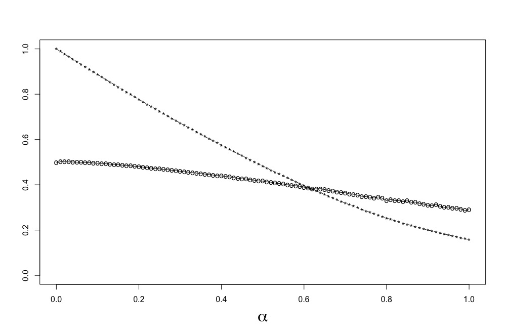
Consider the DAG structure in Figure 6. The Markov boundary of is . Note that since FOCI works in a greedy fashion, it is not hard to build distributions such that FOCI selects earlier than or . For example let
| (8) |
where , and are i.i.d , and is a non-negative constant. We assume for simplicity of exposition that is noiseless. Figure 7 shows the values of and for , with , where follow the SEM in (8). This shows that for small values of , the -Markov Gap assumption (A.3) is not satisfied and FOCI selects earlier than , .
Although FOCI stops after selecting all , therefore, returns a Markov blanket with high probability, this Markov blanket is no longer the Markov boundary. To get to the Markov boundary, one must perform further subset selection which makes the problem more computationally involved.