On the ground-state energy of a mixture of two different oppositely polarized fermionic gases

Whether the ferromagnetic behaviour of a gas of spin $1/2$ fermions (i.e. the emergence of the so-called itinerant ferromagnetism) can be induced by their repulsive spin-independent interaction is experimentally still an open issue which is being studied by exploiting the upper branch of the Feshbach resonance allowing to appropriately tune the interaction strength of fermionic atoms of ultra-cold gases [2, 3]. Theoretical studies of this problem have a long history. The classic mean-field calculation [4] predicts that the critical interaction strength above which the ground state energy $E_{\Omega}$ of the polarized gas of spin $1/2$ fermions is lower than that of the nonpolarized one is $k_{\rm F}a_{0}=\pi/2$, where $k_{\rm F}=3\pi^{2}N/V$ is the gas Fermi vector and $a_{0}$ is the $s$-wave scattering length characterizing the repulsive interaction. More recently computations of the ground-state energy going beyond the mean-field approximation [5], also ones exploiting the quantum Monte Carlo simulations [6], have resulted in a lower critical value, $k_{\rm F}a_{0}\approx 0.8$. This relatively large critical interaction strength seems to be a source of considerable difficulties in experimental observation of the effect [3, 7].

Among different possible ways of favouring the appearance of ferromagnetism the use of a mixture of oppositely polarized different fermionic atomic gases (of different masses) has been proposed. The computation of the ground-state energy of such a mixture in the approximation going one order beyond the simple mean-field one, i.e. up to terms of order $(k_{\rm F}a_{0})^{2}$ has been undertaken in [1] and a variety of possible phases of the system has been exhibited by a detailed numerical study.

The order $(k_{\rm F}a_{0})^{2}$ correction in the perturbative expansion of the ground-state energy $E_{\Omega}$ of interacting fermionic system can be computed either more traditionally, as in [1], by the method outlined in [8] which leads to rather complicated multiple integrals which must be evaluated numerically, or using the effective theory [9] (see also [10, 11] for applications of this method to many-body systems). The latter method is particularly well suited for the case in which the interaction potential is not given explicitly but is from the outset characterized only by the set of scattering lengths $a_{\ell}$ and effective radii $r_{\ell}$, $\ell=0,1,\dots$ It allowed to easily recover [9] the classic order $(k_{\rm F}a_{0})^{2}$ result in the case of a unpolarized gas of identical fermions of arbitrary spin and to extend it up to yet higher orders [9, 12]. Very recently we have used it [13] to obtain the order $(k_{\rm F}a_{0})^{2}$ correction to the ground state energy of the diluted polarized gas of identical spin 1/2 fermions, easily numerically recovering (and thereby demonstrating its universality) the old analytic result of Kanno [14] which has been obtained by the method of [8] for the specific hard-core interaction potential.

It is a natural step to extend the effective theory approach to the case of a diluted mixture of oppositely polarized fermions of different masses. We present this extension in this paper. It turns out that it reduces to only a small modification of the computation done in [13] and as there, part of the computations can be done analytically; the remaining integrals are simple (compared to the ones done in [1]) and can be easily evaluated numerically with the help of a three-line Mathematica code using its standard built-in integration routines. Moreover, the correctness of the computation is partially controlled by the cancellation of ultraviolet divergences. The computation is sketched in Section 2 and the comparison and the discussion are given in Section 3.

If the gas of fermions is diluted, so that the Fermi wave vector $k_{\rm F}=(3\pi^{2}N/V)^{1/3}$ (where $N=N_{a}+N_{b}$) is sufficiently small, its ground-state energy $E_{\Omega}$ can be computed using the effective theory approach [9]. As follows from the analysis done there, to obtain $E_{\Omega}$ up to the order $(k_{\rm F}a_{0})^{2}$, it is sufficient to restrict oneself to the lowest dimension interaction operator, i.e. to consider the Hamiltonian of form¹¹ 1 Since in the considered system there are no $a$-fermions with spin down ($b$-fermions with spin up), the possible interactions of $a$-fermions ($b$-fermions) between themselves do not play any role in determination of $E_{\Omega}$ owing to the Pauli exclusion principle and the nonrelativistic character of the theory (impossibility of particle-antiparticle pair creation) and can, therefore, be omitted.

$\displaystyle H_{\rm eff}=H_{0}+V_{\rm int}=\sum_{\mathbf{p}}\left({\hbar^{2}\mathbf{p}^{2}\over 2m_{a}}~\!a^{\dagger}_{\mathbf{p}}a_{\mathbf{p}}+{\hbar^{2}\mathbf{p}^{2}\over 2m_{b}}~\!b^{\dagger}_{\mathbf{p}}b_{\mathbf{p}}\right)+{C_{0}\over V}\sum_{\mathbf{q}}\sum_{\mathbf{p}_{1},\mathbf{p}_{2}}a^{\dagger}_{\mathbf{p}_{1}+\mathbf{q}}a_{\mathbf{p}_{1}}b^{\dagger}_{\mathbf{p}_{2}-\mathbf{q}}b_{\mathbf{p}_{2}}~\!,$

(2)

(the most general effective Hamiltonian has in principle infinitely many operator structures of growing dimension [9, 10, 11]). In contrast to the underlying “fundamental” Hamiltonian (1), the effective one, (2), is strictly local. The zeroth and first order contributions to $E_{\Omega}$

$\displaystyle E_{\Omega}^{(0)}+E_{\Omega}^{(1)}={V\over 6\pi^{2}}~\!{3\over 5}~\!{\hbar^{2}\over 2}\left({p^{5}_{{\rm F}a}\over m_{a}}+{p^{5}_{{\rm F}b}\over m_{b}}\right)+VC_{0}~\!{p^{3}_{{\rm F}a}\over 6\pi^{2}}~\!{p^{3}_{{\rm F}b}\over 6\pi^{2}}~\!,$

(3)

in which $p_{{\rm F}a/b}=(6\pi^{2}N_{a/b}/V)^{1/3}$ are the Fermi wave-vectors of the $a$- and $b$-fermions, can be then immediately obtained by applying to the Hamiltonian (2) the ordinary Rayleigh-Schrödinger expansion in conjunction with the standard methods of second quantization [16, 17]. The coefficient $C_{0}$ has to be related to the $s$-wave scattering length $a_{0}$ which is extracted from the expansion ($k=|\mathbf{k}|$)

$\displaystyle f(k,\theta)=-a_{0}\left[1-ia_{0}k+\left({1\over 2}~\!a_{0}r_{0}-a_{0}^{2}\right)k^{2}+\dots\right]-a_{1}^{3}k^{2}\cos\theta+\dots,$

(4)

of the amplitude of the elastic scattering of the $a$- and $b$-fermions with the wave vectors $\mathbf{k}_{a}=\mathbf{k}$ and $\mathbf{k}_{b}=-\mathbf{k}$, generated by the interaction $V_{\rm int}$ of (2). The amplitude $f(k,\theta)$ can in turn be obtained from the corresponding $S$-matrix element $S_{\beta\alpha}$ computed in the second quantization formalism with the help of the standard formula [18]

	$\displaystyle S_{\beta\alpha}=\langle\mathbf{k}^{\prime}_{a},\mathbf{k}^{\prime}_{b}|{\rm T}\exp\!\left(-{i\over\hbar}\!\int_{-\infty}^{\infty}\!dt~\!V_{\rm int}^{I}(t)\right)\!|\mathbf{k}_{a},\mathbf{k}_{b}\rangle$		(5)
	$\displaystyle\equiv\delta_{\beta\alpha}-{i\over\hbar}~\!(2\pi)^{4}\delta^{(4)}(k_{a}^{\prime}+k_{a}^{\prime}-k_{a}-k_{b})~\!{\cal A}~\!,~\!$

in which $V_{\rm int}^{I}(t)$ is the interaction picture counterpart of the interaction term of (2) written in the continuum normalization

	$\displaystyle V^{I}_{\rm int}(t)=C_{0}\int\!d^{3}\mathbf{x}~\!\psi^{\dagger}_{a}(t,\mathbf{x})~\!\psi_{a}(t,\mathbf{x})~\!\psi^{\dagger}_{b}(t,\mathbf{x})~\!\psi_{b}(t,\mathbf{x})~\!,$		(6)
	$\displaystyle\psi_{a}(t,\mathbf{x})=\int\!{d^{3}\mathbf{k}\over(2\pi)^{3}}~\!e^{-i\omega^{a}_{\mathbf{k}}t+i\mathbf{k}\cdot\mathbf{x}}~\!a(\mathbf{k})~\!,\phantom{aaaaaaaaaaaa}$

etc. and T is the symbol of the chronological ordering; employed is also the “four-vector” notation in which $k^{0}_{a/b}=\omega^{a/b}_{\mathbf{k}}\equiv\hbar\mathbf{k}^{2}/2m_{a/b}$. The necessary rule is

$\displaystyle f(k,\theta)=-{m_{\rm red}\over 2\pi\hbar^{2}}~\!{\cal A}(k,\theta)~\!,$

(7)

where $m_{\rm red}\equiv m_{a}m_{b}/(m_{a}+m_{b})$ is the reduced mass of the interacting fermions. In the lowest order of the Dyson expansion of (5) one readily finds (see e.g. [9, 10]) that $C_{0}=(2\pi\hbar^{2}/m_{\rm red})a_{0}$. This allows to express (3) - the first nontrivial approximation to the ground-state energy - in terms of a physical quantity $a_{0}$.

The local character of the interaction term of the Hamiltonian (2) results in ultraviolet divergences in higher order corrections, both to the scattering amplitude ${\cal A}$ extracted from (5) and to $E_{\Omega}$; the corrections to the result (3) can be most conveniently computed using the formula²² 2 The symbol T of the chronological ordering should not be confused with $T$ denoting time.

$\displaystyle\lim_{T\rightarrow\infty}\exp(-iT(E_{\Omega}-E_{\Omega_{0}})/\hbar)=\lim_{T\rightarrow\infty}\langle\Omega_{0}|{\rm T}\exp\!\left(-{i\over\hbar}\!\int_{-T/2}^{T/2}\!dt~\!V^{I}_{\rm int}(t)\right)\!|\Omega_{0}\rangle~\!.$

(8)

according to which $(E_{\Omega}-E_{\Omega_{0}})/V$ is directly given by $i\hbar$ times the sum of the momentum space connected vacuum Feynman diagrams (the factor $(2\pi)^{4}\delta^{(4)}(0)$ arising in evaluating connected vacuum diagrams in the position space is interpreted as $VT$). The divergences, if regularized in the same way in evaluating the formulae (5) and (8), disappear from the result for $E_{\Omega}$ when $C_{0}$ and coefficients of other operator structures of the effective Hamiltonian are in it consistently, order by order, traded for the scattering lengths $a_{\ell}$ and the effective ranges $r_{\ell}$ extracted from the computed scattering amplitude.

Here we regularize the divergences by cutting off all integrals over the wave vectors $\mathbf{k}$ at the scale $\Lambda$. The limit $\Lambda\rightarrow\infty$ will be taken after expressing $E_{\Omega}$ computed in terms of $a_{\ell}$ and $r_{\ell}$’s (as in [13] the cancellation of the terms diverging as $\Lambda\rightarrow\infty$ will serve as a partial check of the correctness of the calculation). Thus, to obtain the complete correction $E^{(2)}_{\Omega}$ to the result (3), $C_{0}$ in $E^{(1)}_{\Omega}$ has to be expressed through $a_{0}$ up to one-loop order. The interaction (6) leads to two one-loop diagrams shown in Figs. 1a and 1b, representing scattering of $a$-fermions on $b$-fermions. The second one vanishes, however, owing to the absence of antiparticles; moreover it is easy to see that this interaction generates a whole class of diagrams shown in Fig. 1c which can be easily taken into account. Evaluating them using the standard Feynman rules [16] with the propagators

$\displaystyle\langle{\rm void}|{\rm T}\psi_{a/b}(t,\mathbf{x})\psi^{\dagger}_{a/b}(t^{\prime},\mathbf{x}^{\prime})|{\rm void}\rangle=\int\!{d^{3}\mathbf{k}\over(2\pi)^{3}}~\!e^{i\mathbf{k}\cdot(\mathbf{x}-\mathbf{x}^{\prime})}\!\int\!{d\omega\over 2\pi}~\!{i~\!e^{-i\omega(t-t^{\prime})}\over\omega-\omega^{a/b}_{\mathbf{k}}+i0}~\!,$

one obtains for the scattering amplitude the expression³³ 3 Upon integrating over frequencies with the help of the residue method the denominators of the propagators neatly combine so that the result depends only on $m_{\rm red}$.

$\displaystyle f(k,\theta)=-{m_{\rm red}\over 2\pi\hbar^{2}}~\!C_{0}\left\{1+\left({C_{0}\over i\hbar}\right)\left({2m_{\rm red}\over i\hbar}~\!I_{0}\right)+\left({C_{0}\over i\hbar}\right)^{2}\left({2m_{\rm red}\over i\hbar}~\!I_{0}\right)^{2}+\dots\right\},$

(9)

where

$\displaystyle I_{0}=\int\!{d^{3}\mathbf{q}\over(2\pi)^{3}}~\!{1\over\mathbf{q}^{2}-\mathbf{k}^{2}-i0}~\!.$

(10)

The amplitude (9), supplemented in general with ($k$-dependent) terms which come from diagrams generated by the other interactions (omitted in (2)) of the effective Hamiltonian should be matched onto the expansion (4).

The integral $I_{0}$ is divergent and requires regularization. Imposing the UV cut-off $\Lambda$ on $q=|\mathbf{q}|$ one obtains ($k=|\mathbf{k}|$)

$\displaystyle I_{0}(k,\Lambda)={1\over 4\pi^{2}}\!\int_{0}^{\Lambda}\!dq~\!q\left[{1\over q-k-i0}+{1\over q+k+i0}\right]={i\over 4\pi}~\!k+{1\over 2\pi^{2}}~\!\Lambda-{1\over 2\pi^{2}}~\!{k^{2}\over\Lambda}+\dots,$

(11)

upon using the standard Sochocki formula $1/(x\pm i0)=P(1/x)\mp i\pi\delta(x)$ ($P$ stands for principal value). Inserting this into the formula (9) matched onto the expansion (4) and solving for $C_{0}$ one finds

$\displaystyle C_{0}={2\pi\hbar^{2}\over m_{\rm red}}~\!a_{0}\left(1+{2\over\pi}~\!a_{0}\Lambda+\dots\right).$

(12)

The right hand side of the formula (8) can be evaluated using the standard rules of the many-body quantum field theory (see e.g. [16]). Because $|\Omega_{0}\rangle$ is the lowest energy state of $N_{a}$ free $a$-fermions and $N_{b}$ free $b$-fermions, in the momentum space lines of Feynman diagrams correspond to the propagators

$\displaystyle i\tilde{G}^{(0)}_{a/b}(\omega,\mathbf{k})=i\left[{\theta(|\mathbf{k}|-p_{{\rm F}a/b})\over\omega-\omega^{a/b}_{\mathbf{k}}+i0}+{\theta(p_{{\rm F}a/b}-|\mathbf{k}|)\over\omega-\omega^{a/b}_{\mathbf{k}}-i0}\right].$

(13)

and, to account for the normal ordered form of the interaction term in (2), one has only to add the rule [16] that if a line originates from and ends up in one and the same vertex, the propagator (13) corresponding to this line has to be multiplied by $e^{i\omega\eta}$ with the limit $\eta\rightarrow 0^{+}$ taken at the end.

In the first order in $C_{0}$ there is only one connected vacuum graph shown in Figure 2 which (evaluated in the position space) immediately gives $(iG^{(0)}_{a/b}(0)$ are the propagators (13) written in the position space)

$\displaystyle TE^{(1)}_{\Omega}=C_{0}~\!VT~\!iG^{(0)}_{a}(0)~\!iG^{(0)}_{a}(0)=C_{0}~\!VT~\!{p^{3}_{{\rm F}a}\over 6\pi^{2}}~\!{p^{3}_{{\rm F}b}\over 6\pi^{2}}~\!,$

which reproduces the result (3).

As explained in [9], the only nonzero contribution to the second order correction $E^{(2)}_{\Omega}$ comes from the Feynman diagram shown in Figure 3. Performing the same steps as in the analogous computation [13] of the second order correction to the ground state energy of a polarized system of spin $1/2$ fermions (to which the present computation reduces in the limit of $m_{a}=m_{b}$) one arrives at the expression

$\displaystyle{E^{(2)}_{\Omega}\over V}={C_{0}^{2}\over\hbar}\!\!\int\!{d^{3}\mathbf{q}\over(2\pi)^{3}}\!\!\int\!{d^{3}\mathbf{p}\over(2\pi)^{3}}\!\!\int\!{d^{3}\mathbf{k}\over(2\pi)^{3}}{\theta(p_{{\rm F}a}-|\mathbf{k}|)~\!\theta(p_{{\rm F}b}-|\mathbf{p}|)~\!\theta(|\mathbf{k}+\mathbf{q}|-p_{{\rm F}a})~\!\theta(|\mathbf{p}-\mathbf{q}|-p_{{\rm F}b})\over\omega^{a}_{\mathbf{k}}+\omega^{b}_{\mathbf{p}}-\omega^{a}_{\mathbf{k}+\mathbf{q}}-\omega^{b}_{\mathbf{p}-\mathbf{q}}+i0}~\!.$

The next step is passing to the integrations over the variables $\mathbf{s}$, $\mathbf{t}$ and $\mathbf{u}$ defined by the relations (the Jacobian equals 8):

$\displaystyle\mathbf{k}=\tilde{m}_{a}\mathbf{s}-\mathbf{t}~\!,\phantom{aaa}\mathbf{p}=\tilde{m}_{b}\mathbf{s}+\mathbf{t}~\!,\phantom{aaa}\mathbf{q}=\mathbf{t}-\mathbf{u}~\!,$

which are the appropriate modification of those used in [9, 13], where

$\displaystyle\tilde{m}_{a/b}={2m_{a/b}\over m_{a}+m_{b}}~\!,\phantom{aaaa}\tilde{m}_{a}+\tilde{m}_{b}=2~\!.$

The denominator of the integrand then becomes equal $\hbar(\mathbf{t}^{2}-\mathbf{u}^{2}+i0)/2m_{\rm red}$ and the first and second order corrections to the ground-state energy can be, after using (12), written together in the form

$\displaystyle{E^{(1)}_{\Omega}+E^{(2)}_{\Omega}\over V}={p^{3}_{{\rm F}b}p^{3}_{{\rm F}a}\over 9\pi^{3}}~\!{\hbar^{2}\over 2m_{\rm red}}~\!a_{0}+{2~\!p^{3}_{{\rm F}b}p^{3}_{{\rm F}a}\over 9\pi^{4}}~\!{\hbar^{2}\over 2m_{\rm red}}~\!a^{2}_{0}\Lambda+{\hbar^{2}\over 2m_{\rm red}}~\!256a_{0}^{2}~\!{\tilde{J}\over(2\pi)^{4}}~\!,$

(14)

where ($\tilde{m}_{b}=2-\tilde{m}_{a}$)

	$\displaystyle\tilde{J}(p_{{\rm F}a},p_{{\rm F}b},\tilde{m}_{a})=\int_{0}^{s_{\rm max}}\!ds~\!s^{2}{1\over 4\pi}\!\int\!d^{3}\mathbf{t}~\!\theta(p_{{\rm F}b}-|\mathbf{t}+\tilde{m}_{b}\mathbf{s}|)~\!\theta(p_{{\rm F}a}-|\mathbf{t}-\tilde{m}_{a}\mathbf{s}|)~\!\tilde{g}(t,s)~\!,$		(15)
	$\displaystyle\tilde{g}(t,s)\equiv\tilde{g}(|\mathbf{t}|,s)={1\over 4\pi}\!\int\!d^{3}\mathbf{u}~\!{\theta(|\mathbf{u}+\tilde{m}_{b}\mathbf{s}|-p_{{\rm F}b})~\!\theta(|\mathbf{u}-\tilde{m}_{a}\mathbf{s}|-p_{{\rm F}a})\over\mathbf{t}^{2}-\mathbf{u}^{2}+i0}~\!.\phantom{aaaaa}\!$

The regions of the integrations over $d^{3}\mathbf{u}$ and over $d^{3}\mathbf{t}$ are determined by the intersections of two Fermi spheres of unequal radii, $p_{{\rm F}b}$ and $p_{{\rm F}a}$, the centers of which are displaced from the origin of the $\mathbf{u}$ (of the $\mathbf{t}$) space by the vectors $-\tilde{m}_{b}\mathbf{s}$ ($\mathbf{s}$ will be taken to determine the $z$-axes of the $\mathbf{u}$ and $\mathbf{t}$ spaces in the integrals over $d^{3}\mathbf{u}$ and $d^{3}\mathbf{t}$) and $\tilde{m}_{a}\mathbf{s}$, respectively (the distance between the centers is $2|\mathbf{s}|$). This is the only modification compared to the computation done in [13]. The integral over $\mathbf{u}$ runs over the infinite exterior of these spheres and is, therefore, divergent; the integration over $\mathbf{t}$ covers the interior of their intersection. For this reason the outermost integration over $s\equiv|\mathbf{s}|$ is restricted to $s\leq s_{\rm max}={1\over 2}(p_{{\rm F}a}+p_{{\rm F}b})$ because if $s>s_{\rm max}$, the two spheres which determine the region of the integration over $\mathbf{t}$ become disjoint.

As far as the integral giving $\tilde{g}(t,s)$ is concerned, the range of the variable $s$ splits into two domains: $0\leq s\leq s_{0}={1\over 2}(p_{{\rm F}a}-p_{{\rm F}b})$ and $s_{0}\leq s\leq s_{\rm max}$. Correspondingly, the integral $\tilde{J}$ splits into $\tilde{J}_{1}+\tilde{J}_{2}$.

If $0\leq s\leq s_{0}$, the smaller sphere of radius $p_{{\rm F}b}$ is entirely contained inside the one of radius $p_{{\rm F}a}$ and plays no role in determining the domain of integration over $\mathbf{u}$: this domain is then just the (infinite) exterior of the sphere of radius $p_{{\rm F}a}$ the center of which is at $u_{z}=0$, when $s=0$ and moves to the right as $s$ increases. The computation of $\tilde{g}(t,s)$ for $0\leq s\leq s_{0}$ and of $\tilde{J}_{1}$ proceeds therefore exactly as in the case of equal masses discussed in [13] and one readily finds that

$\displaystyle\tilde{g}(t,s)=g(t,~\!\tilde{m}_{a}s)~\!,\phantom{aaaa}0\leq s\leq s_{0}~\!,$

(16)

where

$\displaystyle g(t,s)=-\Lambda+{1\over 2}~\!p_{{\rm F}a}+{t\over 4}\ln{(p_{{\rm F}a}-t)^{2}-s^{2}\over(p_{{\rm F}a}+t)^{2}-s^{2}}+{p^{2}_{{\rm F}a}-s^{2}-t^{2}\over 8s}\ln{(p_{{\rm F}a}+s)^{2}-t^{2}\over(p_{{\rm F}a}-s)^{2}-t^{2}}~\!.\phantom{a}$

(17)

is the function obtained in [13] in the case of $m_{a}=m_{b}$.

Since $\tilde{J}_{1}$ is obtained by integrating the function $\tilde{g}(t,s)$ first over the interior of the sphere of radius $p_{{\rm F}b}$, the center of which is shifted by $-\tilde{m}_{b}\mathbf{s}$ from the origin of the $\mathbf{t}$ space, and then, with the weight $s^{2}$, over $s$ from 0 to $s_{0}$, it is straightforward to obtain the divergent part $\tilde{J}_{1}^{\rm div}$ of $\tilde{J}_{1}$:

$\displaystyle\tilde{J}^{\rm div}_{1}=-{1\over 9}~\!\Lambda~\!s_{0}^{3}~\!p^{3}_{{\rm F}b}=-{1\over 72}~\!\Lambda~\!(p_{{\rm F}a}-p_{{\rm F}b})^{3}~\!p^{3}_{{\rm F}b}~\!.$

(18)

The finite part of $\tilde{J}_{1}$ can be easily obtained by numerical integration. This can be done either by writing $\mathbf{t}=\mathbf{t}^{\prime}-\tilde{m}_{b}\mathbf{s}$ and introducing the spherical coordinate system in the $\mathbf{t}^{\prime}$ space with the $t^{\prime}_{z}$ axis taken in the direction of the vector $\mathbf{s}$:

$\displaystyle\tilde{J}_{1}={1\over 2}\int_{0}^{s_{0}}\!ds~\!s^{2}\!\int_{-1}^{1}\!d\eta\int_{0}^{p_{{\rm F}b}}\!dt^{\prime}~\!t^{\prime 2}~\!g\!\left(\sqrt{t^{\prime 2}-2t^{\prime}\tilde{m}_{b}s\eta+\tilde{m}_{b}^{2}s^{2}},~\!\tilde{m}_{a}s\right),$

or just by using the Mathematica instruction 0.5NIntegrate$[s^{2}t^{2}g[t,\tilde{m}_{a}s]~\!{\rm Boole}[t^{2}+2t\tilde{m}_{b}sx+\tilde{m}_{b}^{2}s^{2}<p^{2}_{{\rm F}b}],~\!\{s,0,s_{0}\},~\!\{x,-1,1\},~\!\{t,0,\infty\}]$.

We now compute the function $\tilde{g}(t,s)$ for $s_{0}\leq s\leq s_{\rm max}$ and the corresponding contribution $\tilde{J}_{2}$ to the integral (15). In this regime the two Fermi spheres which determine the ranges of integrations over $\mathbf{u}$ and over $\mathbf{t}$ intersect one another. In the $\mathbf{u}$ space the $z$ coordinate $u_{z}^{0}$ of the intersection and its distance $u_{0}$ from the origin are determined by solving the equations

	$\displaystyle u^{2}_{\perp}+(u_{z}-\tilde{m}_{a}s)^{2}=p^{2}_{{\rm F}a}~\!,$
	$\displaystyle u^{2}_{\perp}+(u_{z}+\tilde{m}_{b}s)^{2}=p^{2}_{{\rm F}b}~\!,\phantom{aa}$

which give (recall that $\tilde{m}_{a}+\tilde{m}_{b}=2$)

$\displaystyle u^{0}_{z}=-{1\over 4s}\left(p^{2}_{{\rm F}a}-p^{2}_{{\rm F}b}\right)+{1\over 2}(\tilde{m}_{a}-\tilde{m}_{b})~\!s~\!,\phantom{aaa}u^{2}_{0}={1\over 2}\left(\tilde{m}_{b}p^{2}_{{\rm F}a}+\tilde{m}_{a}p^{2}_{{\rm F}b}\right)-\tilde{m}_{a}\tilde{m}_{b}~\!s^{2}~\!.$

(19)

In the spherical system the “critical” angles $\vartheta_{0}$ corresponding to the intersection of the spheres (marked in Figs. 4) are given by

$\displaystyle\cos\vartheta_{0}=\xi_{0}={u_{z}^{0}\over u_{0}}~\!.$

(20)

Therefore, if $s_{0}\leq s\leq s_{\rm max}$ (i.e. when the two Fermi spheres intersect), the function $\tilde{g}(t,s)$ is given by⁴⁴ 4 Actually this way of computing $\tilde{g}(t,s)$ in this regime ($s_{0}<s<s_{\rm max}$) is justified geometrically only for $s$ not greater than some critical value (depending on the ratios $p_{{\rm F}b}/p_{{\rm F}a}$ and $m_{b}/m_{a}$) which is smaller than $s_{\rm max}$. For $s$ greater than critical, the dashed lines in Fig. 4 pass through the interiors of the smaller spheres and the formula (21) may seem to be unjustified. We have checked, however, by integrating numerically functions over the domain formed by the exterior of the intersecting spheres lying inside a large sphere of radius $R>2p_{{\rm F}a}$ that the formula (21) always gives the correct answer.

$\displaystyle\tilde{g}(t,s)={1\over 2}\int_{-1}^{\xi_{0}}\!d\xi\int_{u_{b}(\xi,s)}^{\Lambda}\!du~\!{u^{2}\over t^{2}-u^{2}+i0}+{1\over 2}\int_{\xi_{0}}^{1}\!d\xi\int_{u_{a}(\xi,s)}^{\Lambda}\!du~\!{u^{2}\over t^{2}-u^{2}+i0}~\!,$

(21)

where $u_{b}(\xi,s)=-\tilde{m}_{b}s~\!\xi+\sqrt{p^{2}_{{\rm F}b}-\tilde{m}_{b}^{2}s^{2}(1-\xi^{2})}$, $u_{a}(\xi,s)=\tilde{m}_{a}s~\!\xi+\sqrt{p^{2}_{{\rm F}a}-\tilde{m}_{a}^{2}s^{2}(1-\xi^{2})}$; of course $u_{b}(\xi_{0},s)=u_{a}(\xi_{0},s)\equiv u_{0}$. After extracting the terms diverging with $\Lambda\rightarrow\infty$ as in [9, 13] (they combine to $-2\pi^{2}I_{0}$ where $I_{0}$ is given in (11)) one gets

$\displaystyle\tilde{g}(t,s)=-\Lambda-i{\pi\over 2}~\!t+{1\over 2}\int_{-1}^{\xi_{0}}\!d\xi\int_{0}^{u_{b}(\xi,s)}\!du~\!{u^{2}\over u^{2}-t^{2}-i0}+{1\over 2}\int_{\xi_{0}}^{1}\!d\xi\int_{0}^{u_{a}(\xi,s)}\!du~\!{u^{2}\over u^{2}-t^{2}-i0}~\!.$

It is now straightforward to compute $\tilde{J}_{2}^{\rm div}$ and to check the cancellation of $\Lambda$. Indeed, the integral

$\displaystyle{1\over 4\pi}\int\!d^{3}\mathbf{t}~\!\theta(p_{{\rm F}b}-|\mathbf{t}+\tilde{m}_{b}\mathbf{s}|)~\!\theta(p_{{\rm F}a}-|\mathbf{t}-\tilde{m}_{a}\mathbf{s}|)(-\Lambda)~\!,$

can be done by shifting the origin of the $\mathbf{t}$-space so that the intersection of the two Fermi spheres occurs at $t_{z}^{\prime}=0$. The integration over $d^{3}\mathbf{t}$ is then easy and its result is

$\displaystyle-{\Lambda\over 2}\left\{\left[{1\over 3}p^{3}_{{\rm F}b}-{1\over 2}p^{2}_{{\rm F}b}(s+u_{z}^{0})+{1\over 6}(s+u_{z}^{0})^{3}\right]+\left[{1\over 3}p^{3}_{{\rm F}a}-{1\over 2}p^{2}_{{\rm F}a}(s-u_{z}^{0})+{1\over 6}(s-u_{z}^{0})^{3}\right]\right\},$

where $u_{z}^{0}$ is given by (19). This should be integrated from $s_{0}={1\over 2}(p_{{\rm F}a}-p_{{\rm F}b})$ to $s_{\rm max}={1\over 2}(p_{{\rm F}a}+p_{{\rm F}b})$ with the weight $s^{2}$. Mathematica does the integration readily with the expected result:

$\displaystyle\tilde{J}_{2}^{\rm div}=-\Lambda\left({p_{{\rm F}a}^{2}p_{{\rm F}b}^{4}\over 24}-{p_{{\rm F}a}p_{{\rm F}b}^{5}\over 24}+{p_{{\rm F}b}^{6}\over 72}\right).$

Combining this with the divergent part (18) of $\tilde{J}_{1}$ one gets

$\displaystyle\tilde{J}_{1}^{\rm div}+\tilde{J}_{2}^{\rm div}=-\Lambda~\!{p_{{\rm F}b}^{3}p_{{\rm F}a}^{3}\over 72}~\!,$

which is precisely what is needed to cancel in (14) the term explicitly proportional to $\Lambda$ which comes from expressing $C_{0}$ in terms of the scattering length in the first order result.

The remaining integrals in $\tilde{g}(t,s)$ can be worked out exactly as in [13] using the trick given in Appendix C of [15], that is by taking the integrals over $\xi$ by parts after inserting into them $1=d\xi/d\xi$. The integrals have imaginary parts which together precisely cancel the imaginary part which arose from the divergent integral $I_{0}$ and the final result for $s_{0}\leq s\leq s_{\rm max}$ is

	$\displaystyle\tilde{g}(t,s)=-\Lambda+{1\over 4}(p_{{\rm F}b}+p_{{\rm F}a}+2s)+{t\over 4}\ln{p_{{\rm F}b}+\tilde{m}_{b}s-t\over p_{{\rm F}b}+\tilde{m}_{b}s+t}+{t\over 4}\ln{p_{{\rm F}a}+\tilde{m}_{a}s-t\over p_{{\rm F}a}+\tilde{m}_{a}s+t}\phantom{aaaaaaaa}$
	$\displaystyle+~\!{p^{2}_{{\rm F}b}-t^{2}-\tilde{m}_{b}^{2}s^{2}\over 8\tilde{m}_{b}s}\ln{(p_{{\rm F}b}+\tilde{m}_{b}s)^{2}-t^{2}\over u_{0}^{2}-t^{2}}+{p^{2}_{{\rm F}a}-t^{2}-\tilde{m}_{a}^{2}s^{2}\over 8\tilde{m}_{a}s}\ln{(p_{{\rm F}a}+\tilde{m}_{a}s)^{2}-t^{2}\over u_{0}^{2}-t^{2}}~\!,\phantom{a}$		(22)

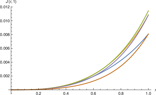
where $u_{0}^{2}$ is given in (19). In the limit $m_{a}=m_{b}$ (i.e. $\tilde{m}_{a}=\tilde{m}_{b}=1$) the results (16) and (22) go over into the ones obtained in [13] which agree with the result obtained in [14]. The finite parts of the functions $\tilde{J}_{1}$ and $\tilde{J}_{2}$, i.e. the integrals over $t$, $\eta$ and $s$, can be easily evaluated using for instance the standard Mathematica function allowing to numerically perform integrations over (multidimensional) domains. Since the finite part of $\tilde{J}=\tilde{J}_{1}+\tilde{J}_{2}$ scales as the seventh power of $p_{{\rm F}a}$, in Fig. 5 we show $\tilde{J}(r,1,\tilde{m}_{a})$ as a function of $r=p_{{\rm F}b}/p_{{\rm F}a}$ for several values of the mass ratio $m_{b}/m_{a}$. It is clear that the curves corresponding to $m_{b}/m_{a}=x$ and $1/x$ merge for $r=1$ (vanishing polarization) as they should; also, independently of the mass ratio, the function $\tilde{J}$ vanishes for the maximal polarization (at $P=1$, i.e. for $r=0$) when all fermions are of the same type, as required by the Pauli exclusion principle.

The energy density with the order $(k_{\rm F}a_{0})^{2}$ term included can be expressed in several equivalent ways. Either in terms of the ratio $r\equiv p_{{\rm F}b}/p_{{\rm F}a}$ and $k_{\rm F}\equiv 3\pi^{2}(N_{a}+N_{b})/V$, so that $p_{{\rm F}a}=k_{\rm F}(2/(1+r^{3}))^{1/3}$,

	$\displaystyle{E_{\Omega}\over V}={k_{\rm F}^{3}\over 3\pi^{2}}~\!{\hbar^{2}k_{\rm F}^{2}\over 4m_{\rm red}}\left({2\over 1+r^{3}}\right)^{5/3}\left\{{3\over 10}\left(\tilde{m}_{b}+\tilde{m}_{a}r^{5}\right)+{2\over 3\pi}~\!r^{3}\left({2\over 1+r^{3}}\right)^{1/3}(k_{\rm F}a_{0})\right.\phantom{aa}$
	$\displaystyle\left.+{96\over\pi^{2}}\left({2\over 1+r^{3}}\right)^{2/3}(k_{\rm F}a_{0})^{2}\tilde{J}(1,r,\tilde{m}_{a})+\dots\right\},~$		(23)

or in terms of the polarization $P=(N_{a}-N_{b})/(N_{a}+N_{b})=(1-r^{3})/(1+r^{3})$

	$\displaystyle{E_{\Omega}\over V}={k_{\rm F}^{3}\over 3\pi^{2}}~\!{\hbar^{2}k_{\rm F}^{2}\over 4m_{\rm red}}\left\{{3\over 10}\left(\tilde{m}_{b}(1+P)^{5/3}+\tilde{m}_{a}(1-P)^{5/3}\right)+{2\over 3\pi}~\!(1-P^{2})~\!(k_{\rm F}a_{0})\right.$
	$\displaystyle\left.+{96\over\pi^{2}}\left(1+P\right)^{7/3}(k_{\rm F}a_{0})^{2}\tilde{J}(1,r(P),\tilde{m}_{a})+\dots\right\},\phantom{aaaaaaaaa}$		(24)

where $r(P)=((1-P)/(1+P))^{1/3}$. Note also that the prefactor $\hbar^{2}k^{5}_{\rm F}/12\pi^{2}m_{\rm red}$ in this formula can be written in the form $(N/V)(\hbar^{2}k^{2}_{\rm F}/4m_{\rm red})$. At zero polarization ($r=1$, $P=0$) the formula (24) simplifies to

$\displaystyle{E_{\Omega}\over V}={k_{\rm F}^{3}\over 3\pi^{2}}~\!{\hbar^{2}k_{\rm F}^{2}\over 4m_{\rm red}}{3\over 5}\left\{1+{10\over 9\pi}~\!(k_{\rm F}a_{0})+{160\over\pi^{2}}~\!(k_{\rm F}a_{0})^{2}\tilde{J}(1,1,\tilde{m}_{a})+\dots\right\}.$

(25)

Setting here $\tilde{m}_{a}=40/23$, i.e. $m_{b}/m_{a}=6/40$, one finds that with $\tilde{J}=0.00808856$ this agrees with the second order result shown for this mass ration in Fig. 1 of [1]. No plots of energy density for nonzero polarization are shown in [1] but the authors give an interpolation formula for the evaluated numerically function $I(P,~\!m_{b}/m_{a})$ in terms of which their second order correction to the system’s energy is expressed. The precise relation of this function $I$ to our function $\tilde{J}$ should be

$\displaystyle{m_{a}+m_{b}\over m_{b}}~\!I(P,~\!m_{b}/m_{a})=320~\!(1+P)^{7/3}~\!\tilde{J}(1,~\!((1-P)/(1+P))^{1/3},~\!2m_{a}/(m_{a}+m_{b}))~\!.$

We have checked that although the interpolation formula of [1] yields for $P=1$ a small but nonzero value of the function $I$ (slightly at variance with the Pauli exclusion principle), it nevertheless agrees excellently with the results of our calculation.

The energy density given by the formula (24) in the case of equal masses ($m_{a}=m_{b}\equiv m_{f}$) of the oppositely polarized fermions is shown in Figure 6. It illustrates the well-known fact [19] that the emergence of a nonzero polarization (of the global minimum of the energy density as a function of $P$) which in the mean-field approximation (i.e. with only the order $k_{\rm F}a_{0}$ term included) is a second order transition [4], after the inclusion of the second order term becomes the first order one. This, however, occurs probably beyond the limits of the reliability of the approximation used: for vanishing polarization the comparison of the second order formula with the results of the quantum Monte Carlo simulations of [6] shows that it is numerically reliable only up to $k_{\rm F}a_{0}\stackrel{{\scriptstyle<}}{{{}_{\sim}}}0.5$.

References

- [1] E. Fratini, S. Pilati, Phys. Rev. A90, 023605 (2014).
- [2] G.-B. Jo, Y.-R. Lee, J.-H. Choi, C.A. Christensen, T.H. Kim, J.H.Thywissen, D.E. Pritchard and W. Ketterle, Science 325 (2009) 1521.
- [3] Y.-R. Lee, M.-S. Heo, J.-H. Choi, T.T. Wang, C.A. Christensen, T.M. Rvachov and W. Ketterle, Phys. Rev. A85 (2012), 063615; C. Sanner, E.J. Su, W. Huang, A. Keshet, J. Gillen and W. Ketterle, Phys. Rev. Lett. 108 (2012), 240404.
- [4] E. Stoner, Philos. Mag. 15, 1018 (1933); see also Section 13.4 in K. Huang, Statistical Mechanics, John Willey and Sons, Inc., New York 1963.
- [5] G.J. Conduit, A.G. Green and B.D. Simons, Phys. Rev. Lett. 103, 207201 (2009); S.-Y. Chang, M. Randeria and N. Trivedi, Proc. Natl. Acad. Sci. USA 108, 51 (2010)
- [6] S. Pilati, G. Bertaina, S. Giorgini and M. Troyer, Phys. Rev. Lett. 105, 030405 (2010), arXiv:1004/1169 [cond-mat.quant-gas].
- [7] D. Pekker, M. Babadi, R. Sensarma, N. Zinner, L. Polleti, W.M. Zwierlein and E. Demler, Phys. Rev. Lett. 106, 050402 (2011).
- [8] A.A. Abrikosov, L.P. Gorkov and I.E. Dzialoshinski, Methods of Quantum Field Theory in Statistical Physics, Dover Publications, Inc. New York, 1975.
- [9] H.-W. Hammer, R. J. Furnstahl, Nucl. Phys. A 678, 277 (2000); arXiv:nucl-th/0004043.
- [10] H.-W. Hammer, S. König and U. van Kolck, Rev. of Mod. Phys. 92 (2020), 025004.
- [11] see e.g. Proceedings of the Joint Caltech/INT Workshop Nuclear Physics with Effective Field Theory, ed. R. Seki, U. van Kolck and M. Savage (World Scientific, 1998); Proceedings of the INT Workshop Nuclear Physics with Effective Field Theory II, ed. P.F. Bedaque, M. Savage, R. Seki and U. van Kolck (World Scientific, 2000).
- [12] C. Wellenhofer, C. Drischler and A. Schwenk, Phys. Lett. B 802 (2020) 135247.
- [13] P. Chankowski and J. Wojtkiewicz, Phys. Rev. B104, 144425 (2021).
- [14] S. Kanno, Prog. Theor. Phys. 44, 813 (1970).
- [15] R. J. Furnstahl, H.-W. Hammer and N. Tirfessa, Nucl. Phys. A 689, 846 (2001).
- [16] A. L. Fetter and J. D. Walecka, Quantum Theory of Many Particle Systems. McGraw Hill, 1971.
- [17] R.P. Feynman, Statistical Mechanics. A Set of Lectures, W.A. Benjamin, Inc. 1972.
- [18] S. Weinberg, The Quantum Theory of Fields, Vol. I, The Press Syndicate of the University of Cambridge, 1995.
- [19] R.A. Duine, A.H. MacDonald, Phys. Rev. Lett. 95, 230403 (2005).