A Causal Approach for Unfair Edge Prioritization and Discrimination Removal

Motivation and Problem: Anti-discrimination laws in the U.S. prohibit unfair treatment of people based on sensitive features, such as gender or race (Act 1964). The fairness of a decision process is based on disparate treatment and disparate impact. Disparate treatment, referred to as intentional discrimination, is when sensitive information is explicitly used to make decisions. Disparate impact, referred to as unintentional discrimination, is when decisions hurt certain sensitive groups even when the policies are neutral. For instance, only candidates with a height of $6$ feet and above are selected for basketball teams. This might eliminate players of a certain race. Unjustifiable disparate impact is unlawful (Barocas and Selbst 2016). In high-risk decisions, such as in the criminal justice system, it is imperative to mitigate unfairness resulting from either disparate treatment or disparate impact. Considering that agencies operate in a budget-constrained scenario owing to limited resources, it is essential to prioritize potential sources of unfairness before we take measures to mitigate them. This paper proposes the Unfair Edge Prioritization methodology for prioritizing these sources before mitigating unfairness during the data generation phase. Further, this paper also proposes the Discrimination Removal procedure to de-bias data distribution after data is generated.

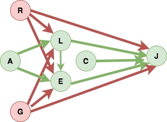
We motivate our problem through the following illustration using Fig. 1. Consider the problem of reducing unfairness in the bail decision $J$ towards a specific racial group $R$. We use an unfair edge as the potential source of unfairness as in Chiappa and Isaac 2018. An unfair path contains at least one unfair edge. The unfairness propagates along all the unfair paths from the racial group $R$ to the bail decision $J$. Although discrimination has been quantified in previous works (Zhang et al. 2017), it only serves as a caution against possible discrimination. There is utility when such notes of caution, like “discrimination exists in the bail decision $J$ towards the racial group $R$”, are augmented with tangible information to mitigate discrimination, like “unfairness in the unfair edge $R\rightarrow L$ is responsible for discrimination in the bail decision $J$ towards the racial group $R$”. Then, the agencies can attempt to address the real-world issues underlying $R\rightarrow L$, such as lack of scholarships for racial group $R$. The challenge lies in providing such tangible information and methodologies for mitigating discrimination such as the amount of unfairness present in an edge, the measure of how edge unfairness affects cumulative unfairness ¹¹ 1 Cumulative unfairness captures discrimination due to unequal influences of $R=r$ on $J=j$ as compared to $R=r^{\prime}$ on $J=j$ via the directed paths from $R$ to $J$., prioritizing the unfair edges, and removing discrimination.

This paper attempts to provide such “tangible” information using Pearl’s framework of Causal Inference (Pearl 2009). The contributions of this paper are as follows,

1. 1.

   Quantify Edge Flow in any edge $X\rightarrow Y$, which is the belief of observing a specific value of $Y$ due to the influence of a specific value of $X$ along the edge $X\rightarrow Y$.

2. 2.

   Quantify Edge Unfairness in any edge $X\rightarrow Y$, which is the average difference in conditional probability of $Y$ given its parents $Pa(Y)$, $\mathbb{P}(Y|Pa(Y))$, with and without edge flow along $X\rightarrow Y$. It measures average unit contribution of edge flow in $X\rightarrow Y$ to $\mathbb{P}(Y|Pa(Y))$. We formulate a non-parametric model for $\mathbb{P}(Y|Pa(Y))$ in terms of edge flows along the parental edges of $Y$ (see Theorem 10).

3. 3.

   Prove that the discrimination in any decision towards any sensitive groups is non-existent when edge unfairness is eliminated. The proof is non-trivial in the non-parametric model setting of CPTs as cumulative unfairness cannot be expressed in terms of edge unfairness. We derive this result by upper bounding the absolute value of cumulative unfairness and showing that the upper bound becomes zero when edge unfairness is zero (see Theorem 12 and Corollary 13).

4. 4.

   Quantify the Potential to Mitigate Cumulative Unfairness by calculating the derivative of the upper bound w.r.t edge unfairness. We do this as cumulative unfairness cannot be expressed in terms of edge unfairness in a non-parametric model setting of CPTs.

5. 5.

   Propose an Unfair Edge Prioritization algorithm to prioritize unfair edges based on their potential to mitigate cumulative unfairness and edge unfairness. Using these priorities, agencies can address the real-world issues underlying the unfair edge with the top priority.

6. 6.

   Propose a Discrimination Removal algorithm to de-bias data distribution by eliminating exponentially growing constraints and subjectively chosen threshold of discrimination.
   

Throughout the paper, we use boldfaced capital letters $\mathbf{X}$ to denote a set of nodes; italicized capital letter $X$ to denote a single node; boldfaced small letters $\mathbf{x}$ to denote a specific value taken by $\mathbf{X}$; italicized small letter $x$ to denote a specific value taken by its corresponding node $X$. $\mathbf{x}_{\mathbf{A}}$ restricts the values of $\mathbf{x}$ to the node-set $\mathbf{A}$. $Pa(X)$ denotes parents of $X$ and $pa(X)$ the specific values taken by them. Each node is associated with the conditional probability table $\mathbb{P}(X|Pa(X))$.

In this section, we quantify edge flow, edge unfairness, prove that eliminating edge unfairness eliminates cumulative unfairness, and quantify the potential to mitigate cumulative unfairness when edge unfairness is reduced.

Edge flow along any edge, say $R\rightarrow J$ is the belief of observing a specific value of bail decision $J$ due to the influence of a specific value of race $R$ along $R\rightarrow J$. This can be extended to multiple direct edges from $\mathbf{M}=\{R,G\}$ to $X$.

Edge flow is formalized using direct effect $SE_{\boldsymbol{\pi},x}(\mathbf{m},\mathbf{m^{\prime}})$ (Avin et al. 2005). $SE_{\boldsymbol{\pi},x}(\mathbf{m},\mathbf{m^{\prime}})$ is the effect of $\mathbf{M=m}$ on $X=x$ along the direct edges from M to $X$ irrespective of the value $\mathbf{m^{\prime}}$ set along the indirect paths ensured by averaging. $SE_{\boldsymbol{\pi},x}(\mathbf{m},\mathbf{m^{\prime}})$ is identifiable because there is no recanting witness (see Definition 3, Theorem 1, and Theorem 2 in Zhang et al. 2017). A positive scaling like softmax ensures that the edge flow is a positive quantity which we use to prove Theorem 12.

To quantify edge unfairness along $R\rightarrow J$, we first decompose $\mathbb{P}(J|Pa(J))$ into edge flows along the direct edges $\{X\rightarrow J|X\in Pa(J)\}$. The rationale is that the active trails $\{X\rightarrow J|X\in Pa(J)\}$ (Definition 6) resulting from the dependencies $\{(J\not\perp X|Pa(J)\backslash X)|X\in Pa(J)\}$, which influence $J$’s value in $\mathbb{P}(J|Pa(J))$ (Theorem 8), are same as the edges along which the edge flows from $Pa(J)$ to $J$ propagate. The theorem below formalizes this concept.

Proof: $\text{FairFlow}_{x,pa(X)}=\mathbb{P}^{pa(X)_{\mathbf{F}_{X}}}_{\text{flow}}(x)$ measures the effect of parents of X along the fair edges and $\text{UnfairFlow}_{x,pa(X)}=\{\mathbb{P}^{A=pa(X)_{A}}_{\text{flow}}(X=x);\penalty\ A\in\mathbf{U}_{X}\}$ measures the effect of parents of X along the unfair edges [Definition 9]. Thus, $\underset{A\in\mathbf{U}_{X}}{\bigcup}\mathbb{P}^{pa(X)_{A}}_{\text{flow}}(x)$ and $\mathbb{P}^{pa(X)_{\mathbf{F}_{X}}}_{\text{flow}}(x)$ measure the effects along the direct edges $\{M\rightarrow X|M\in Pa(X)\}$. Further, the set of active trails resulting from the dependencies $\{(X\not\perp M|Pa(X)\backslash M)|M\in Pa(X)\}$, which influence $X$’s value in $\mathbb{P}(x|pa(X))$, is also $\{M\rightarrow X|M\in Pa(X)\}$ [Theorem 8]. Hence, $\mathbb{P}(x|pa(X))$ can be formulated as a function of $\underset{A\in\mathbf{U}_{X}}{\bigcup}\mathbb{P}^{pa(X)_{A}}_{\text{flow}}(x)$ and $\mathbb{P}^{pa(X)_{\mathbf{F}_{X}}}_{\text{flow}}(x)$ provided the function satisfies the axioms of probability $\blacksquare$.

This theorem aids in the formulation of edge unfairness in an unfair edge, say in $R\rightarrow J$ as the difference in $\mathbb{P}(J|Pa(J))$ with and without the edge flow in $R\rightarrow J$. Edge unfairness is formalized below.

Edge unfairness $\mu_{e}$ is the unit contribution of edge flow $\mathbb{P}^{K}_{\text{flow}}(X)$ to $\mathbb{P}(X|Pa(X))$. $\mu_{e}$ measures the difference in $\mathbb{P}(X|Pa(X))$ with the edge flow along $e$, given by $\text{CPT}^{K}_{x,pa(X)}$, and without the edge flow along $e$, given by $\widetilde{\text{CPT}}^{K}_{x,pa(X)}$. We measure per unit edge flow to capture that a large $D_{X,K}$ compared to $\mathbb{P}^{K}_{\text{flow}}(X)$ still results in large $\mu_{e}$ even though $D^{K}_{X,Pa(X)}$ is small.

Now, we quantify cumulative unfairness. The objective for introducing cumulative (overall) unfairness is twofold: (1)To prove that eliminating edge (local) unfairness eliminates cumulative unfairness (2)To formulate the potential to mitigate cumulative unfairness. We combine direct and indirect discrimination, discussed in Section 3 of Zhang et al. 2017, to define cumulative unfairness towards sensitive nodes $\mathbf{S=s}$ in decision $Y=y$. Cumulative unfairness $C_{\mathbf{S=s},Y=y}$ is,

$C_{\mathbf{S=s},Y=y}$ measures the impact on outcome $Y=y$ when $\mathbf{S}$ is forcibly set to $\mathbf{s}$ along the unfair paths from $\mathbf{S}$ to $Y$ irrespective of the value set along other paths. Since all edges emanating from a sensitive node are potential sources of unfairness, the total causal effect $TE$ (see Definition 4) is used to formulate cumulative unfairness. Proving the result that eliminating edge unfairness $\mu_{e}$ in all unfair edges $e$ eliminates cumulative unfairness $C_{\mathbf{S=s},Y=y}$ is not straightforward as $C_{\mathbf{S=s},Y=y}$ cannot be expressed in terms $\mu_{e}$. We first upper bound $|C_{\mathbf{S=s},Y=y}|$ by $C^{\text{upper}}_{\mathbf{S=s},Y=y}$ that can be expressed in terms of $\mu_{e}$. Then, the result follows from the theorem.

Proof Sketch of Theorem:
Cumulative unfairness $C_{\mathbf{S=s},Y=y}$ cannot be expressed in terms of edge unfairness when the conditional probability is modeled by a non-parametric model $f$. Therefore, we write $C_{\mathbf{S=s},Y=y}$ in terms of conditional probabilities $CPT$s. Each $CPT$ is substituted by its functional model $f$ (see Theorem 10), because the edge unfairness is expressed in terms of $f$ (see Definition 12). To bring edge unfairness $\mu_{e}$ into the formulation, we upper bound each $f$ of a node present along an unfair edge $e$ with the following quantities: edge unfairness $\mu_{e}$ and $f$ having no edge flow along $e$. The rationale of this step comes from the definition of edge unfairness $\mu_{e}$ (see Definition 12) and the fact that the modulus operation is a non-negative quantity. This proves the result $C_{\mathbf{S=s},Y=y}\leq C^{\text{upper}}_{\mathbf{S=s},Y=y}$. By following similar steps and using modulus operation to lower bound $f$, we arrive at $C_{\mathbf{S=s},Y=y}\geq-C^{\text{upper}}_{\mathbf{S=s},Y=y}$. (see Supplementary for full proof) $\blacksquare$

We now measure the potential to mitigate cumulative unfairness when edge unfairness is reduced. Using the potential measure and edge unfairness, agencies can then prioritize the unfair edges before taking measures to mitigate them.

Sensitivity measures the variation in $C^{\text{upper}}_{\mathbf{S=s},Y=y}$ when edge unfairness $\mu_{e}$ in unfair edge $e$ is varied. Since $C^{\text{upper}}_{\mathbf{S=s},Y=y}$ is a linear function in edge unfairness, higher order derivatives ($\geq 2$) of $C^{\text{upper}}_{\mathbf{S=s},Y=y}$ with respect to $\mu_{e}$ are 0.

The following quantity measures the potential to mitigate $C^{\text{upper}}_{\mathbf{S=s},Y=y}$ when edge unfairness $\mu_{e}$ in unfair edge $e$ is decreased. $C^{\text{upper}}_{\mathbf{S=s},Y=y}$ is used to measure the potential contrary to $C_{\mathbf{S=s},Y=y}$ because $C_{\mathbf{S=s},Y=y}$ cannot be expressed in terms of edge unfairness. Experiment 5.3 validates that decreasing $C^{\text{upper}}_{\mathbf{S=s},Y=y}$ decreases $C_{\mathbf{S=s},Y=y}$.

$P^{\mathbf{S=s},Y=y}_{e}$ states that if $C^{\text{upper}}_{\mathbf{S=s},Y=y}=0$, then $C^{\text{upper}}_{\mathbf{S=s},Y=y}$ deviates from 0 (indicative of no-discrimination) as edge unfairness is decreased. The potential of $C^{\text{upper}}_{\mathbf{S=s},Y=y}$ to move towards 0 or to get mitigated is then quantified by $-|S^{\mathbf{S=s},Y=y}_{e}|$ wherein negative is due to $C^{\text{upper}}_{\mathbf{S=s},Y=y}$ deviating from 0. Similarly, one can analyze the other case.

Based on the theorems and the definitions, we present pseudo-codes for fitting the $CPTs$ in Algorithm 1, computing priority of the unfair edges in Algorithm 2, and removing discrimination in Algorithm 3. Algorithm 2 aids the agencies to mitigate unfairness underlying the unfair edges in the real-world during the data generation phase. Algorithm 3 de-biases data distribution after the data generation phase. Algorithm 2 calls Algorithm 1. Algorithm 1 does not call Algorithm 2 and Algorithm 3. Algorithm 3 does not call Algorithm 2 and Algorithm 1.

In this section, we perform experiments to validate the model and input specifications for approximating CPTs using the criminal recidivism graph as shown in Fig. 1. The effectiveness and efficiency of algorithms depend upon their building blocks: (1) Edge Unfairness, (2) Theorem 3, (3) Algorithm 1. Hence, we focus the experimental section on Edge Unfairness formulation, Theorem 12 and Algorithm 1 as they are used in Algorithm 2 and Algorithm 3. In particular, we analyze the relationship between Cumulative Unfairness and the upper bound of Cumulative Unfairness, and the applicability of our method to realistic scenarios where the causal model and the CPTs are unavailable. We first define the causal model by constructing the CPTs.

Mitigating Unfairness in the Data Generation Phase: Gebru et al. 2018 suggests documenting the dataset by recording the motivation and creation procedure. However, it does not attempt to provide a solution for mitigation with limited resources.

Assumptions: Zhang et al. 2017 assumes that the sensitive variable $S$ has no parents as it is an inherent nature of the individual. We follow Zhang et al. 2019 that relaxes this assumption because sensitive nodes such as religious belief can have parents like literacy $L$. Nabi and Shpitser 2018 and Chiappa 2019 propose discrimination removal procedures in the continuous node setting by handling the non-identifiability issues. We do not discuss the continuous variable setting to avoid digressing into the intractability issues. Wu et al. 2019 formulates cumulative unfairness as a solution to the optimization problem for the semi-markovian setting. We restrict our discussion to the markovian setting to avoid digressing into the challenges of formulating cumulative unfairness in terms of edge unfairness. Ravishankar et al. 2020 solves the problem for the trivial linear case when the cumulative unfairness can be expressed in terms of edge unfairness.

Edge Flow: Decomposing direct parental dependencies of a child into independent contributions from each of its parents helps in quantifying the edge flow. Srinivas 1993, Kim and Pearl 1983, and Henrion 2013 separate the independent contributions by using unobserved nodes in the representation of causal independence. To overcome the issues of intractability in unobserved nodes, Heckerman 1993 proposed a temporal definition of causal independence. It states that if and only cause $c$ transitions from time $t$ to $t+1$, then the effect’s distribution at time $t+1$ depends only on the effect and the cause at time $t$, and the cause at time $t+1$. Based on this definition, a belief network representation is constructed with the observed nodes that make the probability assessment and inference tractable. Heckerman and Breese 1994 proposes a temporal equivalent of the temporal definition of Heckerman 1993. The aforementioned works do not quantify the direct dependencies from the parents onto the child as in our work.

Edge Unfairness: Multiple statistical criteria have been proposed to identify discrimination (Berk et al. 2018) but it is mathematically incompatible to satisfy them all when base rates of the dependent variable differ across groups (Chouldechova 2017; Kleinberg et al. 2016). Consequently, there is an additional task of selecting which criterion has to be achieved. Moreover, statistical criteria caution about discrimination but do not help in identifying the sources of unfairness. Zhang et al. 2017 uses path-specific effects to identify direct and indirect discrimination after data is generated but does not address the problem of mitigating unfairness in the data generation phase. Unlike Zhang et al. 2017 that uses the presence of a redlining attribute in an indirect path and the presence of a sensitive node on a direct path to determine the unfairness of a path, our work uses the notion of an unfair edge as the potential source of unfairness akin to Chiappa and Isaac 2018.

Discrimination Removal Procedure: Zhang et al. 2017 and Kusner et al. 2017 remove discrimination by altering the data distribution. Firstly, the optimization technique in Zhang et al. 2017 and the sampling procedure in Kusner et al. 2017, scale exponentially in the number of nodes (and values taken by the sensitive nodes) that eventually increases the time to solve the quadratic programming problem. Secondly, the constraints in Zhang et al. 2017 depend on a subjectively chosen threshold of discrimination that is disadvantageous because the regenerated data distribution would remain unfair had a smaller threshold been chosen. Our paper formulates a discrimination removal procedure without exponentially growing constraints and a threshold of discrimination.

We introduce the problem of quantifying edge unfairness in an unfair edge. We give a novel formulation that models $CPTs$ in terms of edge flows to quantify edge unfairness. We prove a result that eliminating edge unfairness eliminates cumulative unfairness. Proving this result is not straightforward because cumulative unfairness cannot be expressed in terms of edge unfairness when $CPTs$ are modeled as a non-parametric function of the edge flows. Hence, we prove the result via an intermediate theorem that upper bounds the magnitude of cumulative unfairness by a quantity that can be expressed in terms of edge unfairness. To analyze the impact of edge unfairness on cumulative unfairness, we quantify the potential to mitigate cumulative unfairness when edge unfairness is decreased. This formulation uses the upper bound of cumulative unfairness as it can be expressed in terms of edge unfairness. Experimental results validate that mitigating cumulative unfairness mitigates its upper bound as well, thereby establishing the rationale for using the upper bound of cumulative unfairness in the formulation. Using the theorem result and measures, we present an unfair edge prioritization algorithm and a discrimination removal algorithm. The unfair edge prioritization algorithm gives tangible directions to agencies to mitigate unfairness in the real world while the data is being generated. There is no utility in making cautionary claims of potential discrimination when it is not complemented with information that aids in mitigating unfairness causing discrimination. On the other hand, the discrimination removal algorithm de-biases data after the data is generated. In the future, we aim to evaluate the impact of edge unfairness on subsequent stages of the machine learning pipeline such as selection, classification, etc. We also plan to extend to the semi-Markovian causal model (Wu et al. 2019) and continuous nodes settings (Nabi and Shpitser 2018).

References

- Act (1964) Civil Rights Act. Civil rights act of 1964. Title VII, Equal Employment Opportunities, 1964.
- Avin et al. (2005) Chen Avin, Ilya Shpitser, and Judea Pearl. Identifiability of path-specific effects. 2005.
- Barocas and Selbst (2016) Solon Barocas and Andrew D Selbst. Big data’s disparate impact. Calif. L. Rev., 104:671, 2016.
- Berk et al. (2018) Richard Berk, Hoda Heidari, Shahin Jabbari, Michael Kearns, and Aaron Roth. Fairness in criminal justice risk assessments: The state of the art. Sociological Methods & Research, page 0049124118782533, 2018.
- Chiappa (2019) Silvia Chiappa. Path-specific counterfactual fairness. In Proceedings of the AAAI Conference on Artificial Intelligence, volume 33, pages 7801–7808, 2019.
- Chiappa and Isaac (2018) Silvia Chiappa and William S Isaac. A causal bayesian networks viewpoint on fairness. In IFIP International Summer School on Privacy and Identity Management, pages 3–20. Springer, 2018.
- Chouldechova (2017) Alexandra Chouldechova. Fair prediction with disparate impact: A study of bias in recidivism prediction instruments. Big data, 5(2):153–163, 2017.
- Gebru et al. (2018) Timnit Gebru, Jamie Morgenstern, Briana Vecchione, Jennifer Wortman Vaughan, Hanna Wallach, Hal Daumeé III, and Kate Crawford. Datasheets for datasets. arXiv preprint arXiv:1803.09010, 2018.
- Heckerman (1993) David Heckerman. Causal independence for knowledge acquisition and inference. In Uncertainty in Artificial Intelligence, pages 122–127. Elsevier, 1993.
- Heckerman and Breese (1994) David Heckerman and John S Breese. A new look at causal independence. In Uncertainty Proceedings 1994, pages 286–292. Elsevier, 1994.
- Henrion (2013) Max Henrion. Practical issues in constructing a bayes’ belief network. arXiv preprint arXiv:1304.2725, 2013.
- Kim and Pearl (1983) JinHyung Kim and Judea Pearl. A computational model for causal and diagnostic reasoning in inference systems. In International Joint Conference on Artificial Intelligence, pages 0–0, 1983.
- Kingma and Ba (2014) Diederik P Kingma and Jimmy Ba. Adam: A method for stochastic optimization. arXiv preprint arXiv:1412.6980, 2014.
- Kleinberg et al. (2016) Jon Kleinberg, Sendhil Mullainathan, and Manish Raghavan. Inherent trade-offs in the fair determination of risk scores. arXiv preprint arXiv:1609.05807, 2016.
- Koller and Friedman (2009) Daphne Koller and Nir Friedman. Probabilistic graphical models: principles and techniques. MIT press, 2009.
- Kusner et al. (2017) Matt J Kusner, Joshua R Loftus, Chris Russell, and Ricardo Silva. Counterfactual fairness. arXiv preprint arXiv:1703.06856, 2017.
- Nabi and Shpitser (2018) Razieh Nabi and Ilya Shpitser. Fair inference on outcomes. In Thirty-Second AAAI Conference on Artificial Intelligence, 2018.
- Paszke et al. (2019) Adam Paszke et al. Pytorch: An imperative style, high-performance deep learning library. In H. Wallach, H. Larochelle, A. Beygelzimer, F. d'Alché-Buc, E. Fox, and R. Garnett, editors, Advances in Neural Information Processing Systems 32, pages 8024–8035. Curran Associates, Inc., 2019.
- Pearl (2009) Judea Pearl. Causality. Cambridge university press, 2009.
- Ramsey et al. (2018) Joseph D Ramsey, Kun Zhang, Madelyn Glymour, Ruben Sanchez Romero, Biwei Huang, Imme Ebert-Uphoff, Savini Samarasinghe, Elizabeth A Barnes, and Clark Glymour. Tetrad—a toolbox for causal discovery. In 8th International Workshop on Climate Informatics, 2018.
- Ravishankar et al. (2020) Pavan Ravishankar, Pranshu Malviya, and Balaraman Ravindran. A causal linear model to quantify edge unfairness for unfair edge prioritization and discrimination removal. arXiv e-prints, pages arXiv–2007, 2020.
- Srinivas (1993) Sampath Srinivas. A generalization of the noisy-or model. In Uncertainty in artificial intelligence, pages 208–215. Elsevier, 1993.
- VanderWeele and Staudt (2011) Tyler J VanderWeele and Nancy Staudt. Causal diagrams for empirical legal research: a methodology for identifying causation, avoiding bias and interpreting results. Law, Probability & Risk, 10(4):329–354, 2011.
- Wu et al. (2019) Yongkai Wu, Lu Zhang, Xintao Wu, and Hanghang Tong. Pc-fairness: A unified framework for measuring causality-based fairness. In Advances in Neural Information Processing Systems, pages 3404–3414, 2019.
- Zhang et al. (2019) L. Zhang, Y. Wu, and X. Wu. Causal modeling-based discrimination discovery and removal: Criteria, bounds, and algorithms. IEEE Transactions on Knowledge and Data Engineering, 31(11):2035–2050, 2019.
- Zhang et al. (2017) Lu Zhang, Yongkai Wu, and Xintao Wu. A causal framework for discovering and removing direct and indirect discrimination. In Proceedings of the Twenty-Sixth International Joint Conference on Artificial Intelligence, 2017.
Title: A Causal Approach for Unfair Edge Prioritization and Discrimination Removal
Supplementary Material
1. Choices for
We present two instances for . The list is not limited to these and can be extended as long as satisfies the constraints of the conditional probability (Eq. 9, 10).
- 1.
is a linear combination in the inputs where,
(22) (23) (24) and are constrained between 0 and 1 since the objective of the mapper is to capture the interaction between the fraction of the beliefs given by and and approximate . Eq. 23 and Eq. 24 ensure that the conditional probability axioms of are satisfied.
- 2.
is composite function representing a N-layer neural network with layer having neurons and weights capturing the non-linear combination of the inputs where,
(25) subject to, (26) (27) captures the interaction between and and models . Eq. 26 and Eq. 27 ensure that the conditional probability axioms of are satisfied. One possibility is to use a softmax function for to ensure that the outputs of satisfy probability axioms.
2. Proof of Theorem 12 & Corollary 13
Proof of Theorem 12