Pessimistic Model Selection for Offline Deep Reinforcement Learning
Abstract
Deep Reinforcement Learning (DRL) has demonstrated great potentials in solving sequential decision making problems in many applications. Despite its promising performance, practical gaps exist when deploying DRL in real-world scenarios. One main barrier is the over-fitting issue that leads to poor generalizability of the policy learned by DRL. In particular, for offline DRL with observational data, model selection is a challenging task as there is no ground truth available for performance demonstration, in contrast with the online setting with simulated environments. In this work, we propose a pessimistic model selection (PMS) approach for offline DRL with a theoretical guarantee, which features a provably effective framework for finding the best policy among a set of candidate models. Two refined approaches are also proposed to address the potential bias of DRL model in identifying the optimal policy. Numerical studies demonstrated the superior performance of our approach over existing methods.
1 Introduction
The success of deep reinforcement learning (Mnih et al. 2013; Henderson et al. 2018) (DRL) often leverages upon executive training data with considerable efforts to select effective neural architectures. Deploying online simulation to learn useful representations for DRL is not always realistic and possible especially in some high-stake environments, such as automatic navigation (Kahn et al. 2018; Hase et al. 2020), dialogue learning (Jaques et al. 2020), and clinical applications (Tang et al. 2020a). Offline reinforcement learning (Singh & Sutton 1996; Levine et al. 2020; Agarwal et al. 2020) (OffRL) has prompted strong interests (Paine et al. 2020; Kidambi et al. 2020) to empower DRL toward training tasks associated with severe potential cost and risks. The idea of OffRL is to train DRL models with only logged data and recorded trajectories. However, with given observational data, designing a successful neural architecture in OffRL is often expensive (Levine et al. 2020), requiring intensive experiments, time, and computing resources.
Unlike most aforementioned applications with online interaction, Offline tasks for reinforcement learning often suffer the challenges from insufficient observational data from offline collection to construct a universal approximated model for fully capturing the temporal dynamics. Therefore, relatively few attempts in the literature have been presented for provide a pipeline to automate the development process for model selection and neural architecture search in OffRL settings. Here, model selection refers to selecting the best model (e.g., the policy learned by a trained neural network) among a set of candidate models (e.g. different neural network hyperparameters).
In this work, we propose a novel model selection approach to automate OffRL development process, which provides an evaluation mechanism to identify a well-performed DRL model given offline data. Our method utilizes statistical inference to provide uncertainty quantification on value functions trained by different DRL models, based on which a pessimistic idea is incorporated to select the best model/policy. In addition, two refined approaches are further proposed to address the possible biases of DRL models in identifying the optimal policy. In this work, we mainly focus on deep Q-network (Mnih et al. 2013; Mnih et al. 2015) (DQN) based architectures, while our proposed methods can be extended to other settings. Figure 1 demonstrates the superior performance of the proposed pessimistic model selection (PMS) method in identifying the best model among DRL models of different algorithms on one navigation task (See Appendix C for details), compared with the model selection method by (Tang & Wiens 2021) which uses three offline policy evaluation (OPE) estimates for validation. Specifically, based on the derived confidence interval of the OPE value for each candidate model, the final selected model by our PMS method is the one that has the largest lower confidence limit, which exactly has the largest true OPE value among all candidate models. In contrast, none of three OPE estimates used for model selection by Tang & Wiens 2021 can identify the best model due to the inevitable overfitting issue during the validation procedure.
To close this section, we summarize the contributions of this work as follows:
- •
We propose a novel PMS framework, which targets finding the best policy from given candidate models (e.g., neural architecture, hyperparameters, etc) with offline data for DQN learning. Unlike many existing methods, our approach essentially does not involve additional hyperparameter tuning except for two interpretable parameters.
- •
Leveraging asymptotic analysis in statistical inference, we provide uncertainty quantification on each candidate model, based on which our method can guarantee that the worst performance of finally selected model is the best among all candidate models. See Corollary 1 for more details.
- •
To address potential biases of candidate models in identifying the optimal policy, two refined approaches are proposed, one of which can be shown to have regret bounded by the smallest error bound among all candidate models under some technical conditions (See Corollary 2). To the best of our knowledge, this is the first model-selection method in offline DRL with such a guarantee.
- •
The numerical results demonstrate that the proposed PMS shows superior performance in different DQN benchmark environments.
2 Related Work
Model Selection for Reinforcement Learning: Model selection has been studied in online decision-making environments (Fard & Pineau 2010; Lee & Taylor 2014). Searching nearly optimal online model is a critical topic for online bandits problems with limited information feed-backs. For linear contextual bandits, Abbasi-Yadkori et al. 2011; Chu et al. 2011 are aiming to find the best worst-case bound when the optimal model class is given. For model-based reinforcement learning, Pacchiano et al. 2020 introduces advantages of using noise augmented Markov Decision Processes (MDP) to archive a competitive regret bound to select an individual model with constraints for ensemble training. Recently, Lee et al. 2021 utilized an online algorithm to select a low-complexity model based on a statistical test. However, most of the previous model selection approaches are focused on the online reinforcement learning setting. Very few works including Farahmand & Szepesvári 2011; Paine et al. 2020; Su et al. 2020; Yang et al. 2020b; Kuzborskij et al. 2021; Tang & Wiens 2021; Xie & Jiang 2021 are focused on the offline setting. In particular, (Su et al. 2020; Yang et al. 2020b; Kuzborskij et al. 2021) focus on model selection for OPE problem. (Farahmand & Szepesvári 2011; Xie & Jiang 2021) select the best model/policy based on minimizing the Bellman error, while the first approach requires an additional tuning and latter does not. (Paine et al. 2020; Tang & Wiens 2021) proposed several criteria to perform model selection in OffRL and mainly focused on numerical studies. In this work, we provide one of the first model selection approaches based on statistical inference for RL tasks with offline data collection.
Offline-Policy Learning: Training a DRL agent with offline data collection often relies on batch-wise optimization. Batch-Constrained deep Q-learning (Fujimoto et al. 2019) (BCQ) is considered one OffRL benchmark that uses a generative model to minimize the distance of selected actions to the batch-wise data with a perturbation model to maximize its value function. Other popular OffRL approaches, such as behavior regularized actor-critic (BRAC) (Wu et al. 2019), and random ensemble mixture (Agarwal et al. 2020) (REM) (as an optimistic perspective on large dataset), have also been studied in RL Unplugged (RLU) (Gulcehre et al. 2020) benchmark together with behavior cloning (Bain & Sammut 1995; Ross & Bagnell 2010) (BC), DQN, and DQN with quantile regression (Dabney et al. 2018) (QR-DQN). RLU suggests a naive approach based on human experience for offline policy selection, which requires independent modification with shared domain expertise (e.g., Atari environments) for tuning each baseline. Meanwhile, how to design a model selection algorithm for OffRL remains an open question. Motivated by the benefits and the challenges as mentioned earlier of the model selection for offline DRL, we aim to develop a unified approach for model selection in offline DRL with theoretical guarantee and interpretable tuning parameters.
3 Background and Notations
Consider a time-homogeneous Markov decision process (MDP) characterized by a tuple , where is the state space, is the action space, is the transition kernel, i.e., is the probability mass (density) of transiting to given current state-action , is the reward function, i.e., for , and is a discount factor. For simplifying presentation, we assume and are both finite. But our method can also be applied in continuous cases. Under this MDP setting, it is sufficient to consider stationary Markovian policies for optimizing discounted sum of rewards (Puterman 1994). Denote as a stationary Markovian policy mapping from the state space into a probability distribution over the action space. For example, denotes the probability of choosing action given the state value . One essential goal of RL is to learn an optimal policy that maximizes the value function. Define and then the optimal policy is defined as , where denotes some reference distribution function over . In addition, we denote Q-function as for and . In this work, we consider the OffRL setting. The observed data consist of trajectories, corresponding to independent and identically distributed copies of . For any , data collected from the th trajectory can be summarized by , where denotes the termination time. We assume that the data are generated by some fixed stationary policy denoted by .
Among many RL algorithms, we focus on Q-learning type of methods. The foundation is the optimal Bellman equation given below.
| (1) |
where is called optimal Q-function, i.e., Q-function under . Among others, fitted q-iteration (FQI) is one of the most popular RL algorithms (Ernst et al. 2005). FQI leverages supervised learning techniques to iteratively solve the optimal Bellman equation (1) and shows competitive performance in OffRL.
To facilitate our model-selection algorithm, we introduce the discounted visitation probability, motivated by the marginal importance sampling estimator in (Liu et al. 2018). For any , let denote the -step visitation probability assuming the actions are selected according to at time . We define the discounted visitation probability function as . To adjust the distribution from behavior policy to any target policy , we use the discounted probability ratio function defined as
| (2) |
where is the -step visitation probability under the behavior policy , i.e., . The ratio function is always assumed well defined. The estimation of ratio function is motivated by the observation that for every measurable function defined over ,
| (3) |
based on which several min-max estimation methods has been proposed such as (Liu et al. 2018; Nachum et al. 2019; Uehara & Jiang 2019); We refer to (Uehara & Jiang 2019, Lemma 1) for a formal proof of equation (3).
Finally, because our proposed model selection algorithm relies on an efficient evaluation of any target policy using batch data, we introduce three types of offline policy evaluation estimators in the existing RL literature. The first type is called direct method via estimating Q-function, based on the relationship that . The second type is motivated by the importance sampling (Precup 2000). Based on the definition of ratio function, we can see , from which a plugin estimator can be constructed. The last type of OPE methods combines the first two types of methods and construct a so-called doubly robust estimator (Kallus & Uehara 2019; Tang et al. 2020b). This estimator is motivated by the efficient influence function of under a transition-sampling setting and the model that consists of the set of all observed data distributions given by arbitrarily varying the initial, transition, reward, and behavior policy distributions, subject to certain minimal regularity and identifiability conditions (Kallus & Uehara 2019), i.e.,
| (4) |
A nice property of doubly robust estimators is that as long as either the Q-function or the ratio function can be consistently estimated, the final estimator of is consistent (Robins et al. 1994; Jiang & Li 2015; Kallus & Uehara 2019; Tang et al. 2020b). Furthermore, a doubly robust estimator based on (3) can achieve semiparametric efficiency under the conditions proposed by (Kallus & Uehara 2019), even if nuisance parameters are estimated via black box models such as deep neural networks. Therefore such an estimator is particularly suitable under the framework of DRL. Our proposed algorithm will rely on this doubly robust type of OPE estimator.
4 Pessimistic Model Selection (PMS) for Best Policy
In this section, we discuss our pessimistic model selection approach. For the ease of presentation, we focus on the framework of (deep) Q-learning, where policy optimization is performed via estimating the optimal Q-function. While this covers a wide range of state-of-the-art RL algorithms such as FQI (Ernst et al. 2005), DQN (Mnih et al. 2013) and QR-DQN (Dabney et al. 2018), we remark that our method is not restricted to this class of algorithms.
Suppose we have total number of candidate models for policy optimization, where each candidate model will output an estimated policy, say for . Our goal is to select the best policy among policies during our training procedure. Note that these models can be different deep neural network architectures, hyper-parameters, and various classes of functions for approximating the optimal Q-function or policy class, etc.
4.1 Difficulties and Challenges
Given a candidate among models, we can apply for example FQI using the whole batch data to learn an estimate of as and an estimated optimal policy defined as for every . In order to select the final policy, one may use a naive greedy approach to choose some such that as our goal is to maximize . However, using this criterion will lead to over-fitting. Specifically, due to the distributional mismatch between the behavior policy and target policies, which is regarded as a fundamental challenge in OffRL (Levine et al. 2020), we may easily overestimate Q-function, especially when some state-action pairs are not sufficiently visited in the batch data. This issue becomes more serious when we apply max-operator during our policy optimization procedure. Such observations have already been noticed in recent works, such as (Kumar et al. 2019; Kumar et al. 2020; Paine et al. 2020; Yu et al. 2020; Tang & Wiens 2021; Jin et al. 2021). Therefore, it may be inappropriate to use this criterion for selecting the best policy among models.
One may also use cross-validation procedure to address the issue of over-fitting or overestimating Q-function for model selection. For example, one can use OPE approaches on the validate dataset to evaluate the performance of estimated policies from the training data set (see Tang & Wiens 2021 for more details). However, since there is no ground truth for the value function of any policies, the OPE procedure on the validation dataset cannot avoid involving additional tuning on hyperparameters. Therefore such a procedure may still incur a large variability due to the over-fitting issue. In addition, arbitrarily splitting the dataset for cross-validation and ignoring the Markov dependent structure will cause additional errors, which should be seriously taken care of.
4.2 Sequential Model Selection
In the following, we propose a pessimistic model selection algorithm for finding an optimal policy among candidate models. Our goal is to develop an approach to estimate the value function under each candidate model during our policy optimization procedure with theoretical guarantee. The proposed algorithm is motivated by recent development in statistical inference of sequential decision making (Luedtke & Van Der Laan 2016; Shi et al. 2020). The idea is to first estimate optimal Q-function , optimal policy and the resulting ratio function based on a chunk of data, and evaluate the performance of the estimated policy on the next chunk of data using previously estimated nuisance functions. Then we combine the first two chunks of data, perform the same estimation procedure and evaluation on the next chunk of data. The framework of MDP provides a nature way of splitting the data.
Specifically, denote the index of our batch dataset as . We divide into number of non-overlapping subsets, denoted by and the corresponding data subsets are denoted by . Without loss of generality, we assume these data subsets have equal size. We require that for any , any and , either or . For , denote the aggregate chunks of data as
We focus on FQI algorithm for illustrative purpose and it should be noticed that our algorithm can be applied to other RL algorithms. Starting from the first chunk of our batch data, at the -th step (, for each candidate model , we apply FQI on to compute as an estimate of optimal Q-function and obtain correspondingly such that for every . Additionally, we compute an estimate of ratio function using by many existing algorithms such as Nachum et al. 2019. Denote the resulting estimator as . The purpose of estimating this ratio function is to improve the efficiency and robustness of our value function estimation for each candidate model. Then we compute the estimated value function of on as
| (5) | ||||
| (6) |
where denotes the empirical average over the chunk of dataset and is one transition tuple in . While one can aggregate for to evaluate the performance of models, the uncertainty of these estimates due to the finite sample estimation should not be ignored. Therefore, in the following, we derive an uncertainty quantification of our estimated value function for each candidate model, for performing model selection. Based on equation (3), (conditioning on ), the variance of is
| (7) |
where is a transition tuple with follows some stationary distribution. See Assumption 1. Correspondingly we have an estimate defined as
| (8) |
The estimation procedure stops once we have used all our offline data and denote the final estimated policy as for each . Notice that . Finally, we compute the weighted average of all the intermediate value functions as our final evaluation of the estimated policy , i.e.,
| (9) |
In Section 5, we show that under some technical conditions, the following asymptotic result holds:
| (10) |
where , refers to weak convergence when either or goes to infinity, and refers to the standard normal distribution. Based on the asymptotic result in (10), we can construct a confidence interval for the value function of each policy . Given a confidence level , for each , we can compute , where is -quantile of the standard normal distribution. Our final selected one is .
The use of is motivated by the recent proposed pessimistic idea to address the overestimation issue of value (or Q) function in the OffRL setting. See Kumar et al. 2019; Kumar et al. 2020; Jin et al. 2021; Xie et al. 2021; Uehara & Sun 2021; Zanette et al. 2021 for details. The final output of our algorithm is and an outline of the proposed algorithm can be found in Algorithm 1. As we can see, our algorithm is nearly tuning free, which provides great flexibility in real-world applications. The only two adjustable parameters is and . The size of balances the computational cost and the finite-sample accuracy of evaluating each candidate model. In specific, we can indeed show that the variance of the estimated value function by our algorithm can achieve the semi-parametric efficiency bound, which is best one can hope for. So in the asymptotic sense, the effect of is negligible. In the finite-sample setting, we believe the performance will be discounted by a factor . Therefore, if is large enough, will have a mere effect on the performance. See Theorem 1. However, using large will result in a large computational cost. As a sacrifice for the nearly tuning free algorithm, we need to apply OffRL algorithms times for each candidate model. The parameter determines how worst the performance of each policy we should use to evaluate each policy. See Corollary 1 for more insights.
2 Compute using by Nachum et al. 2019 and min-max solver for (3).
2 Compute and using given in (5) and (8) respectively.
end for 3
5 Theoretical Results
In this section, we justify our asymptotic result given in (10). We use to denote the stochastic boundedness. Before that, we make several technical assumptions:
Assumption 1
The stochastic process is stationary with stationary distribution .
Assumption 2
For every and , we have for some constant and .
Assumption 1 is standard in the existing literature such as (Kallus & Uehara 2019). Assumption 2 is key to our developed asymptotic results developed. This assumption essentially states that all candidate models are good enough so that eventually their value functions will converge to that of the optimal one. This implies that there is no asymptotic bias in identifying the optimal policy. While this is reasonable thanks to the capability of deep neutral networks, which has demonstrated their empirical success in many RL applications, such an assumption could still be strong. In Section 6, we try to relax this assumption and provide two remedies for addressing possibly biased estimated policies. In addition, Assumption 1 also requires that the convergence rates of value functions under estimated policies are fast enough. This has been shown to hold under the margin condition on , see e.g., (Hu et al. 2021) for more details.
Assumption 3
For every and , suppose for some constant . In addition, is uniformly bounded almost surely.
Assumption 4
For every and , suppose for some constant . In addition, both and are uniformly bounded above and below away from almost surely.
Assumption 5
For every and , and are bounded above and below from almost surely.
Assumptions 3 and 4 impose high-level conditions on two nuisance functions. Our theoretical results only require , which is a mild assumption. For example, if considered parametric models for both Q-function and ratio function, then . If considered nonparametric models for these two nuisance functions such as deep neural networks, then can be obtained under some regularity conditions. See Fan et al. 2020 and Liao et al. 2020; Uehara et al. 2021 for the convergence rates of Q-function and ratio function by non-parametric models respectively. In addition, Assumption 5 is a mild assumption, mainly for theoretical justification. Then we have the following main theorem as a foundation of our proposed algorithm.
Theorem 1 provides an uncertainty quantification of each candidate model used in policy optimization. Such uncertainty quantification is essential in OffRL as data are often limited. We highlight the importance of such results in Appendix A. A consequent result following Theorem 1 validates the proposed Algorithm 1:
As can be seen clearly from Corollary 1 and the proposed PMS, with a large probability (by letting small), we consider the worst performance of each candidate model in the sense of the lower confidence limit of the value function, and then select the best one among all models.
6 Two Refined Approaches
In this section, we relax Assumption 2 by allowing possibly non-negligible bias in estimating the optimal policy and introduce two refined approaches for addressing this issue. Instead of imposing Assumption 2, we make an alternative assumption below.
Assumption 6
For every , there exists such that almost surely.
Assumption 6 is a very mild assumption. It essentially states that the biases for all our intermediate value function estimates are bounded by some constant, which is much weaker than Assumption 2. In this case, the asymptotic results in (11) may not hold in general. Correspondingly, we have the following result.
Motivated by Lepski’s principle (Lepski & Spokoiny 1997) from nonparametric statistics and (Su et al. 2020) studying the model selection of OPE, we consider the following refined model-selection procedure to find the best policy. We first rank candidate models in an non-increasing order based on the value of , i.e., for , . Then for -th model, we construct an interval as Finally the optimal model/policy we choose is such that To show this procedure is valid, we need to make one additional assumption.
Assumption 7
There exists a such that for , and almost surely.
This assumption is borrowed from Su et al. 2020. It typically assumes that after sorting our model based on , the bias of estimated policy is monotonically increasing and the standard deviation is monotonically deceasing but not too quickly. This is commonly seen when all candidate estimators exhibit some bias-variance trade-off phenomena. Define the following event
| (13) |
Then we have the following theoretical guarantee for our refined procedure.
Corollary 2
The additional assumption (i.e., the high probability bound) in Corollary 2 can be shown to hold by the empirical process theory under some technical conditions (Van de Geer 2000). Hence Corollary 2 provides a strong guarantee that the regret of the final selected policy is bounded by the smallest error bound among all candidate policies. Note that Assumption 3 imposed here could be strong.
Another refined approach: Notice that the above refined approach indeed focuses on OPE estimates to select the best policy with regret warranty. The rough motivation behind is to find a policy that has the smallest estimation error to the optimal one. However, such procedure may not directly match the goal of maximizing the value function in OffRL. To relieve this issue , we can alternatively choose the final policy as such that where the argmax is taken over models. This approach can be viewed as a combination of PMS and the above refined approach. By adopting this approach, candidate models with large biases are firtly removed by the truncation on . Then, we use the idea of PMS to select the best model having the best worst performance among the remaining candidates. Unfortunately, we do not have theoretical guarantee for this combined approach.
7 Experimental Results
We select six DQN environments ( to ) from open-source benchmarks (Brockman et al. 2016; Juliani et al. 2018) to conduct numerical experiments, as shown in Fig. 5 of Appendix C. These tasks of deployed environments cover different domains that include tabular learning (Fig 5(a)); automatic navigation in a geometry environment with a physical ray-tracker (Fig 5(b)); Atari digital gaming (Fig 5(c) and (d)), and continuous control (Fig 5(e) and (f)). We provide detailed task description and targeted reward for each environment in Appendix C.
Experiment setups. To evaluate the performance of PMS with DQN models in offRL, we choose different neural network architectures under five competitive DRL algorithms including DQN by (Mnih et al. 2013; Mnih et al. 2015), BCQ by (Fujimoto et al. 2019), BC by (Bain & Sammut 1995; Ross & Bagnell 2010), BRAC by (Wu et al. 2019) from RLU benchmarks, and REM by (Agarwal et al. 2020). Within each architecture, 70 candidate models are created by assigning different hyperparameters and training setups. See Appendix C.1 for details. We then conduct performance evaluation of different OffRL model selection methods on these generated candidate models.

Evaluation procedure. We utilize validation scores from OPE for each model selection algorithm, which picks the best (or a good) policy from the candidate set of size based on its own criterion. Regret is used as the evaluation metric for each candidate. The regret for model is defined as , where corresponds to the candidate policy with the best OPE validation performance. In our implementation, we treat as , the oracle but unknown best possible policy. A small regret is desirable after model selection. Note the optimal regret is not zero since we can only use data to obtain instead of for each model. We provide additional top-k regret and precision results from Figure 6 to 16 in Appendix C.
Performance comparison. As highlighted in Fig. 1 in the introduction, we report estimated OPE values by different model selection approaches, i.e. PMS and three methods by (Tang & Wiens 2021), versus the true OPE values. In this experiment, we consider 70 DQN models under the above mentioned five DRL algorithms, i.e., models are considered for each architecture. We use fewer models for each DRL algorithm mainly for clear presentation. By using the confidence interval constructed by our PMS procedure, our method is able to correctly select the top models, while the other three methods fail. To further investigate the performance of PMS, we implement model selection among models within each DRL algorithm separately. Fig. 2 shows the box plots of averaged regret over six environments after OPE per neural network architecture. Each subfigure contains results from one particular DRL algorithm with different hyperparameters or training setups. The left box plot refers to the regrets of all models and the right one represents the regrets of top models selected by the proposed PMS method. Note that the right box plot is a subset of the left one. The results show that our proposed PMS successfully helps to select models with the best policies and improve the average regret by a significant margin. In particular, PMS-REM-based models attain the lowest regrets, due to the benefit from its ensemble process. Detailed results for each environment is given in Appendix C, where and are used in all experiments.

Sensitivity analysis. Fig. 3 compares different selection algorithms with varying training data size. PMS outperforms others across all scales, and larger number of episodes gives smaller variation and lower sensitivity.
PMS algorithm with refinements. We replicate our experiments on in the offline navigation task in (Banana Collector) for 30 times and report regrets of top models selected by PMS and two refinements in Fig. 4. As we can see, while the overall performances of the proposed three model selection methods are similar, two refined approaches have better regrets than PMS in terms of median, demonstrating their promising performances in identifying the best model. OPE results have been also evaluated also in DRL tasks with and to , where the refinement algorithms (PMS R1/R2) have only a small relative 0.423 % performance difference compared to its original PMS setups.
8 Conclusion
We propose a new theory-driven model selection framework (PMS) for offline deep reinforcement learning based on statistical inference. The proposed pessimistic mechanism is warrants that the worst performance of the selected model is the best among all candidate models. Two refined approaches are further proposed to address the biases of DRL models. Extensive experimental results on six DQN environments with various network architectures and training hyperparameters demonstrate that our proposed PMS method consistently yields improved model selection performance over existing baselines. The results suggest the effectiveness of PMS as a powerful tool toward automating model selection in offline DRL.
References
- Abbasi-Yadkori et al. (2011) Yasin Abbasi-Yadkori, Dávid Pál, and Csaba Szepesvári. Improved algorithms for linear stochastic bandits. Advances in neural information processing systems, 24:2312–2320, 2011.
- Agarwal et al. (2020) Rishabh Agarwal, Dale Schuurmans, and Mohammad Norouzi. An optimistic perspective on offline reinforcement learning. In International Conference on Machine Learning, pp. 104–114. PMLR, 2020.
- Bain & Sammut (1995) Michael Bain and Claude Sammut. A framework for behavioural cloning. In Machine Intelligence 15, pp. 103–129, 1995.
- Barth-Maron et al. (2018) Gabriel Barth-Maron, Matthew W Hoffman, David Budden, Will Dabney, Dan Horgan, TB Dhruva, Alistair Muldal, Nicolas Heess, and Timothy Lillicrap. Distributed distributional deterministic policy gradients. In International Conference on Learning Representations, 2018.
- Bennett & Kallus (2021) Andrew Bennett and Nathan Kallus. Proximal reinforcement learning: Efficient off-policy evaluation in partially observed markov decision processes. arXiv preprint arXiv:2110.15332, 2021.
- Brockman et al. (2016) Greg Brockman, Vicki Cheung, Ludwig Pettersson, Jonas Schneider, John Schulman, Jie Tang, and Wojciech Zaremba. Openai gym. arXiv preprint arXiv:1606.01540, 2016.
- Chen et al. (2021) Xiaocong Chen, Lina Yao, Julian McAuley, Guanglin Zhou, and Xianzhi Wang. A survey of deep reinforcement learning in recommender systems: A systematic review and future directions. arXiv preprint arXiv:2109.03540, 2021.
- Chu et al. (2011) Wei Chu, Lihong Li, Lev Reyzin, and Robert Schapire. Contextual bandits with linear payoff functions. In Proceedings of the Fourteenth International Conference on Artificial Intelligence and Statistics, pp. 208–214. JMLR Workshop and Conference Proceedings, 2011.
- Dabney et al. (2018) Will Dabney, Mark Rowland, Marc Bellemare, and Rémi Munos. Distributional reinforcement learning with quantile regression. In Proceedings of the AAAI Conference on Artificial Intelligence, volume 32, 2018.
- Ernst et al. (2005) Damien Ernst, Pierre Geurts, Louis Wehenkel, and L. Littman. Tree-based batch mode reinforcement learning. Journal of Machine Learning Research, 6:503–556, 2005.
- Fan et al. (2020) Jianqing Fan, Zhaoran Wang, Yuchen Xie, and Zhuoran Yang. A theoretical analysis of deep q-learning. In Learning for Dynamics and Control, pp. 486–489. PMLR, 2020.
- Farahmand & Szepesvári (2011) Amir-massoud Farahmand and Csaba Szepesvári. Model selection in reinforcement learning. Machine learning, 85(3):299–332, 2011.
- Fard & Pineau (2010) M Fard and Joelle Pineau. Pac-bayesian model selection for reinforcement learning. Advances in Neural Information Processing Systems, 23:1624–1632, 2010.
- Freedman (1975) David A Freedman. On tail probabilities for martingales. the Annals of Probability, pp. 100–118, 1975.
- Fujimoto et al. (2019) Scott Fujimoto, David Meger, and Doina Precup. Off-policy deep reinforcement learning without exploration. In International Conference on Machine Learning, pp. 2052–2062. PMLR, 2019.
- Gottesman et al. (2018) Omer Gottesman, Fredrik Johansson, Joshua Meier, Jack Dent, Donghun Lee, Srivatsan Srinivasan, Linying Zhang, Yi Ding, David Wihl, Xuefeng Peng, et al. Evaluating reinforcement learning algorithms in observational health settings. arXiv preprint arXiv:1805.12298, 2018.
- Gulcehre et al. (2020) Caglar Gulcehre, Ziyu Wang, Alexander Novikov, Tom Le Paine, Sergio Gomez Colmenarejo, Konrad Zolna, Rishabh Agarwal, Josh Merel, Daniel Mankowitz, Cosmin Paduraru, et al. Rl unplugged: Benchmarks for offline reinforcement learning. arXiv e-prints, pp. arXiv–2006, 2020.
- Hase et al. (2020) Hannes Hase, Mohammad Farid Azampour, Maria Tirindelli, Magdalini Paschali, Walter Simson, Emad Fatemizadeh, and Nassir Navab. Ultrasound-guided robotic navigation with deep reinforcement learning. In 2020 IEEE/RSJ International Conference on Intelligent Robots and Systems (IROS), pp. 5534–5541. IEEE, 2020.
- Henderson et al. (2018) Peter Henderson, Riashat Islam, Philip Bachman, Joelle Pineau, Doina Precup, and David Meger. Deep reinforcement learning that matters. In Proceedings of the AAAI conference on artificial intelligence, volume 32, 2018.
- Hu et al. (2021) Yichun Hu, Nathan Kallus, and Masatoshi Uehara. Fast rates for the regret of offline reinforcement learning. arXiv preprint arXiv:2102.00479, 2021.
- Jaques et al. (2020) Natasha Jaques, Judy Hanwen Shen, Asma Ghandeharioun, Craig Ferguson, Agata Lapedriza, Noah Jones, Shixiang Gu, and Rosalind Picard. Human-centric dialog training via offline reinforcement learning. In Proceedings of the 2020 Conference on Empirical Methods in Natural Language Processing (EMNLP), pp. 3985–4003, 2020.
- Jiang & Li (2015) Nan Jiang and Lihong Li. Doubly robust off-policy value evaluation for reinforcement learning. arXiv preprint arXiv:1511.03722, 2015.
- Jin et al. (2021) Ying Jin, Zhuoran Yang, and Zhaoran Wang. Is pessimism provably efficient for offline rl? In International Conference on Machine Learning, pp. 5084–5096. PMLR, 2021.
- Juliani et al. (2018) Arthur Juliani, Vincent-Pierre Berges, Ervin Teng, Andrew Cohen, Jonathan Harper, Chris Elion, Chris Goy, Yuan Gao, Hunter Henry, Marwan Mattar, et al. Unity: A general platform for intelligent agents. arXiv preprint arXiv:1809.02627, 2018.
- Kahn et al. (2018) Gregory Kahn, Adam Villaflor, Bosen Ding, Pieter Abbeel, and Sergey Levine. Self-supervised deep reinforcement learning with generalized computation graphs for robot navigation. In 2018 IEEE International Conference on Robotics and Automation (ICRA), pp. 5129–5136. IEEE, 2018.
- Kallus & Uehara (2019) Nathan Kallus and Masatoshi Uehara. Efficiently breaking the curse of horizon: Double reinforcement learning in infinite-horizon processes. arXiv preprint arXiv:1909.05850, 2019.
- Kidambi et al. (2020) Rahul Kidambi, Aravind Rajeswaran, Praneeth Netrapalli, and Thorsten Joachims. Morel: Model-based offline reinforcement learning. In NeurIPS, 2020.
- Kumar et al. (2019) Aviral Kumar, Justin Fu, Matthew Soh, George Tucker, and Sergey Levine. Stabilizing off-policy q-learning via bootstrapping error reduction. In Advances in Neural Information Processing Systems, pp. 11784–11794, 2019.
- Kumar et al. (2020) Aviral Kumar, Aurick Zhou, George Tucker, and Sergey Levine. Conservative q-learning for offline reinforcement learning. arXiv preprint arXiv:2006.04779, 2020.
- Kuzborskij et al. (2021) Ilja Kuzborskij, Claire Vernade, Andras Gyorgy, and Csaba Szepesvári. Confident off-policy evaluation and selection through self-normalized importance weighting. In International Conference on Artificial Intelligence and Statistics, pp. 640–648. PMLR, 2021.
- Le et al. (2019) Hoang Le, Cameron Voloshin, and Yisong Yue. Batch policy learning under constraints. In International Conference on Machine Learning, pp. 3703–3712, 2019.
- Lee & Taylor (2014) Jason D Lee and Jonathan E Taylor. Exact post model selection inference for marginal screening. In Proceedings of the 27th International Conference on Neural Information Processing Systems-Volume 1, pp. 136–144, 2014.
- Lee et al. (2021) Jonathan Lee, Aldo Pacchiano, Vidya Muthukumar, Weihao Kong, and Emma Brunskill. Online model selection for reinforcement learning with function approximation. In International Conference on Artificial Intelligence and Statistics, pp. 3340–3348. PMLR, 2021.
- Lepski & Spokoiny (1997) Oleg V Lepski and Vladimir G Spokoiny. Optimal pointwise adaptive methods in nonparametric estimation. The Annals of Statistics, pp. 2512–2546, 1997.
- Levine et al. (2020) Sergey Levine, Aviral Kumar, George Tucker, and Justin Fu. Offline reinforcement learning: Tutorial, review, and perspectives on open problems. arXiv preprint arXiv:2005.01643, 2020.
- Liao et al. (2020) Peng Liao, Zhengling Qi, and Susan Murphy. Batch policy learning in average reward markov decision processes. arXiv preprint arXiv:2007.11771, 2020.
- Liu et al. (2018) Qiang Liu, Lihong Li, Ziyang Tang, and Dengyong Zhou. Breaking the curse of horizon: Infinite-horizon off-policy estimation. In Advances in Neural Information Processing Systems, pp. 5356–5366, 2018.
- Luedtke & Van Der Laan (2016) Alexander R Luedtke and Mark J Van Der Laan. Statistical inference for the mean outcome under a possibly non-unique optimal treatment strategy. Annals of statistics, 44(2):713, 2016.
- Mathé (2006) Peter Mathé. The lepskii principle revisited. Inverse problems, 22(3):L11, 2006.
- McLeish (1974) Donald L McLeish. Dependent central limit theorems and invariance principles. the Annals of Probability, 2(4):620–628, 1974.
- Mnih et al. (2013) Volodymyr Mnih, Koray Kavukcuoglu, David Silver, Alex Graves, Ioannis Antonoglou, Daan Wierstra, and Martin Riedmiller. Playing atari with deep reinforcement learning. arXiv preprint arXiv:1312.5602, 2013.
- Mnih et al. (2015) Volodymyr Mnih, Koray Kavukcuoglu, David Silver, Andrei A Rusu, Joel Veness, Marc G Bellemare, Alex Graves, Martin Riedmiller, Andreas K Fidjeland, Georg Ostrovski, et al. Human-level control through deep reinforcement learning. nature, 518(7540):529–533, 2015.
- Nachum et al. (2019) Ofir Nachum, Yinlam Chow, Bo Dai, and Lihong Li. Dualdice: Behavior-agnostic estimation of discounted stationary distribution corrections. In Advances in Neural Information Processing Systems, pp. 2315–2325, 2019.
- Pacchiano et al. (2020) Aldo Pacchiano, Philip Ball, Jack Parker-Holder, Krzysztof Choromanski, and Stephen Roberts. On optimism in model-based reinforcement learning. arXiv preprint arXiv:2006.11911, 2020.
- Paine et al. (2020) Tom Le Paine, Cosmin Paduraru, Andrea Michi, Caglar Gulcehre, Konrad Zolna, Alexander Novikov, Ziyu Wang, and Nando de Freitas. Hyperparameter selection for offline reinforcement learning. arXiv preprint arXiv:2007.09055, 2020.
- Precup (2000) Doina Precup. Eligibility traces for off-policy policy evaluation. Computer Science Department Faculty Publication Series, pp. 80, 2000.
- Puterman (1994) Martin L Puterman. Markov Decision Processes: Discrete Stochastic Dynamic Programming. John Wiley & Sons, Inc., 1994.
- Robins et al. (1994) James M. Robins, Andrea Rotnitzky, and Lue Ping Zhao. Estimation of regression coefficients when some regressors are not always observed. Journal of the American Statistical Association, 89(427):846–866, 1994. ISSN 01621459. URL http://www.jstor.org/stable/2290910.
- Ross & Bagnell (2010) Stéphane Ross and Drew Bagnell. Efficient reductions for imitation learning. In Proceedings of the thirteenth international conference on artificial intelligence and statistics, pp. 661–668. JMLR Workshop and Conference Proceedings, 2010.
- Schaul et al. (2015) Tom Schaul, John Quan, Ioannis Antonoglou, and David Silver. Prioritized experience replay. arXiv preprint arXiv:1511.05952, 2015.
- Shi et al. (2020) Chengchun Shi, Sheng Zhang, Wenbin Lu, and Rui Song. Statistical inference of the value function for reinforcement learning in infinite horizon settings. arXiv preprint arXiv:2001.04515, 2020.
- Siegel et al. (2019) Noah Siegel, Jost Tobias Springenberg, Felix Berkenkamp, Abbas Abdolmaleki, Michael Neunert, Thomas Lampe, Roland Hafner, Nicolas Heess, and Martin Riedmiller. Keep doing what worked: Behavior modelling priors for offline reinforcement learning. In International Conference on Learning Representations, 2019.
- Singh & Sutton (1996) Satinder P Singh and Richard S Sutton. Reinforcement learning with replacing eligibility traces. Machine learning, 22(1):123–158, 1996.
- Su et al. (2020) Yi Su, Pavithra Srinath, and Akshay Krishnamurthy. Adaptive estimator selection for off-policy evaluation. In International Conference on Machine Learning, pp. 9196–9205. PMLR, 2020.
- Tang & Wiens (2021) Shengpu Tang and Jenna Wiens. Model selection for offline reinforcement learning: Practical considerations for healthcare settings. arXiv preprint arXiv:2107.11003, 2021.
- Tang et al. (2020a) Shengpu Tang, Aditya Modi, Michael Sjoding, and Jenna Wiens. Clinician-in-the-loop decision making: Reinforcement learning with near-optimal set-valued policies. In International Conference on Machine Learning, pp. 9387–9396. PMLR, 2020a.
- Tang et al. (2020b) Ziyang Tang, Yihao Feng, Lihong Li, Dengyong Zhou, and Qiang Liu. Doubly robust bias reduction in infinite horizon off-policy estimation. In International Conference on Learning Representations, 2020b.
- Uehara & Jiang (2019) Masatoshi Uehara and Nan Jiang. Minimax weight and q-function learning for off-policy evaluation. arXiv preprint arXiv:1910.12809, 2019.
- Uehara & Sun (2021) Masatoshi Uehara and Wen Sun. Pessimistic model-based offline rl: Pac bounds and posterior sampling under partial coverage. arXiv preprint arXiv:2107.06226, 2021.
- Uehara et al. (2021) Masatoshi Uehara, Masaaki Imaizumi, Nan Jiang, Nathan Kallus, Wen Sun, and Tengyang Xie. Finite sample analysis of minimax offline reinforcement learning: Completeness, fast rates and first-order efficiency. arXiv preprint arXiv:2102.02981, 2021.
- Van de Geer (2000) Sara Van de Geer. Empirical Processes in M-estimation, volume 6. Cambridge university press, 2000.
- Van Hasselt et al. (2016) Hado Van Hasselt, Arthur Guez, and David Silver. Deep reinforcement learning with double q-learning. In Proceedings of the AAAI conference on artificial intelligence, volume 30, 2016.
- Voloshin et al. (2019) Cameron Voloshin, Hoang M Le, Nan Jiang, and Yisong Yue. Empirical study of off-policy policy evaluation for reinforcement learning. arXiv preprint arXiv:1911.06854, 2019.
- Wu et al. (2019) Yifan Wu, George Tucker, and Ofir Nachum. Behavior regularized offline reinforcement learning. arXiv preprint arXiv:1911.11361, 2019.
- Xie & Jiang (2021) Tengyang Xie and Nan Jiang. Batch value-function approximation with only realizability. In International Conference on Machine Learning, pp. 11404–11413. PMLR, 2021.
- Xie et al. (2021) Tengyang Xie, Ching-An Cheng, Nan Jiang, Paul Mineiro, and Alekh Agarwal. Bellman-consistent pessimism for offline reinforcement learning. arXiv preprint arXiv:2106.06926, 2021.
- Yang et al. (2020a) Chao-Han Huck Yang, Jun Qi, Pin-Yu Chen, Yi Ouyang, I-Te Danny Hung, Chin-Hui Lee, and Xiaoli Ma. Enhanced adversarial strategically-timed attacks against deep reinforcement learning. In ICASSP 2020-2020 IEEE International Conference on Acoustics, Speech and Signal Processing (ICASSP), pp. 3407–3411. IEEE, 2020a.
- Yang et al. (2021) Chao-Han Huck Yang, I Hung, Te Danny, Yi Ouyang, and Pin-Yu Chen. Causal inference q-network: Toward resilient reinforcement learning. arXiv preprint arXiv:2102.09677, 2021.
- Yang et al. (2020b) Mengjiao Yang, Bo Dai, Ofir Nachum, George Tucker, and Dale Schuurmans. Offline policy selection under uncertainty. arXiv preprint arXiv:2012.06919, 2020b.
- Yu et al. (2020) Tianhe Yu, Garrett Thomas, Lantao Yu, Stefano Ermon, James Zou, Sergey Levine, Chelsea Finn, and Tengyu Ma. Mopo: Model-based offline policy optimization. arXiv preprint arXiv:2005.13239, 2020.
- Zanette et al. (2021) Andrea Zanette, Martin J Wainwright, and Emma Brunskill. Provable benefits of actor-critic methods for offline reinforcement learning. arXiv preprint arXiv:2108.08812, 2021.
Appendix A Comments on Asymptotic Results
We remark here that all theoretical justification in this paper is based on asymptotics. It might be possible to investigate finite sample regimes when one has an exact confidence interval instead of (11) or a non-asymptotic bound. However, having an exact confidence interval might require some model specification of the value function, and using non-asymptotic bounds might require additional tuning steps (e.g., constants in many concentration inequalities), which is beyond the scope of this paper. In addition, as seen from our empirical evaluations below, with a relatively large sample size, the proposed model selection approach performs well.
Appendix B Technical Proofs
Notations: The notation (resp. ) means that there exists a sufficiently large (resp. small) constant (resp. ) such that (resp. ) for some sequences and related to . In the following proofs, often refers to some quantity related to and .
Lemma 1 and its proof : Let denotes some index of our batch data . Define
where is the cardinality of the index set , e.g., for every . Then we have the following Lemma 1 as an intermediate result to Theorem 1.
Lemma 1
The proof is similar to that of Theorem 7 in Kallus & Uehara 2019. First, notice that
Then it suffices to show the term in the first bracket converges to faster than . Notice that
where
and
Next, we bound each of the above three terms. For term , it can be seen that
In addition, by Assumptions 3 and 4, we can show
where the inequality is based on that each item in is uncorrelated with others. Then by Markov’s inequality, we can show
Similarly, we can show
For term , by Cauchy Schwarz inequality and similar arguments as before, we can show
Therefore, as long as , we have , which concludes our proof.
Proof of Theorem 1 We aim to show that
It can be seen that
Define
where is the cardinality of the index set , i.e., . Then by Lemma 1, we show that
| (16) |
If we can show that
which will be shown later, then by Slutsky theorem, we can show that
For , we can see that
| (17) | ||||
| (18) |
By the sequential structure of our proposed algorithm, forms a mean zero martingale. Then we use Corollary 2.8 of (McLeish 1974) to show its asymptotic distribution. First of all, by the uniformly bounded assumption on Q-function, ratio function and the variance, we can show that
Next, we aim to show that
| (19) | ||||
Notice that the left hand side of the above is bounded above by
| (20) | ||||
| (21) |
Because, for each ,
| (22) | ||||
| (23) | ||||
| (24) |
forms a mean zero martingale, we apply Freedman’s inequality in (Freedman 1975) with Assumptions 3-5 to show it is bounded by . Applying union bound shows (19) is and furthermore consistency of in (16) holds. Then we apply the martingale central limit theorem to show
The remaining is to show
is asymptotically negligible. Consider
| (25) | ||||
| (26) | ||||
| (27) | ||||
| (28) |
where we use Assumption 2 for the last inequality. Summarizing together, we can show that
where we obtain the second inequality by that . In the last inequality, we use in Assumption 2. Then Markov inequality gives that
Moreover, by Assumption 5 that for some constant , we can further show that
which completes our proof.
Proof of Corollary 1 Denote the sets , , where . Note that and
where the last inequality holds because given the event , one has and for any . This completes the proof by taking on both sides.
Proof of Theorem 2 To show the results in Theorem 2, it can be seen that
Then by results in the proof of Theorem 1, we can show that
| (29) |
This implies that
| (30) | ||||
| (31) |
which concludes our proof.
Proof of Corollary 2: We mainly show the proof of the second claim in the corollary, based on which the first claim can be readily seen. Define an event such that , and . Based on the assumption given in Corollary 2 and Theorem 2, we have . In the following, we suppose event holds.
Inspired by the proofs of Corollary 1 in (Mathé 2006) and Theorem 3 of (Su et al. 2020), we define , where . Let . By Assumption 7, for ,
which further implies that for any ,
Then based on the construction of for all . In addition, we have for
| (32) |
by triangle inequality and event . Since share at least one common element for , we have . Moreover, there must exist an element such that , where and . This indicates that
| (33) | ||||
| (34) |
by again triangle inequality and Assumption 7, and
| (35) |
by event and Assumption 7. Define . Then following the similar proof of (Su et al. 2020), we consider two cases:
Appendix C More Details on DQN Environments

We introduce our deployed DQN environments in this section, which included four environments with discrete action ( to ) and two environments ( to ) with continuous action. These environments cover wide applications, including tabular learning (), navigation to a target object in a geometrical space (), digital gaming ( to ), and continuous control ( to ).


: Frozen Lake: The Frozen Lake is a maze environment that manipulates an agent to walk from a starting point (S) to a goal point without failing into the hole (H). We use FrozenLake-v0 from OpenAI Gym (Brockman et al. 2016) as shown in Fig 5(a). We provide top-5 regret and precision results shown in Figure 6 and 7.
: Banana Collector: The Banana collector is one popular 3D-graphical navigation environment that compresses discrete actions and states as an open source DQN benchmark from Unity 11 1 https://www.youtube.com/watch?v=heVMs3t9qSk ML-Agents v0.3.(Juliani et al. 2018). The DRL agent controls an automatic vehicle with 37 dimensions of state observations including velocity and a ray-based perceptional information from objects around the agent. The targeted reward is points by accessing correct yellow bananas () and avoiding purple bananas () in first-person point of view as shown in Fig 5(b). We provide the related top-5 regret and precision results shown in Figure 8 and 9.


: Pong: Pong is one Atari game environment from OpenAI Gym (Brockman et al. 2016) as shown in Fig 5(c). We provide its top-5 regret and precision results shown in Figure 10 and 11.


: Breakout: Breakout is one Atari game environment from OpenAI Gym (Brockman et al. 2016) as shown in Fig 12(d). We provide the related top-5 regret and precision results shown in Figure 12 and 13.
: HalfCheetah-v1: Halfcheetah is a continuous action and state environment to control agent with monuments made by MuJoCo simulators as shown in Fig 5(e). We provide the related top-5 regret and precision results shown in Figure 14 and 15.
: Walker2d-v1: Walker2d-v1 is a continuous action and state environment to control agent with monuments made by MuJoCo simulators as shown in Fig 5(f). We provide the related top-5 regret and precision results shown in Figure 16 and 17.
C.1 Hyper-Parameters Information
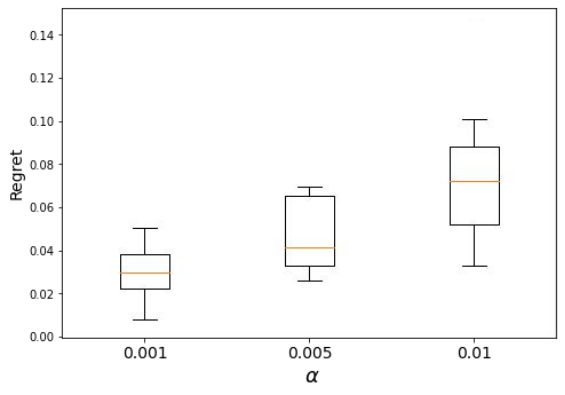
We select a total of DQN based models for each environment. We will open source the model and implementation for future studies. Table 1, Table 2, and Table 3 summarize their hyper-parameter and setups. In addition, Figure 18 and Figure 19 provide ablation studies on different scales of and selection in PMS experiments for the deployed DRL navigation task (). From the experimental results, a more pessimistic (e.g., 0.001) is associated with a slightly better attained top-5 regret. Meanwhile, the selection of does not produce much different performance on selected policies but slightly affects the range of the selected policies.
| Hyper-parameters | Values |
|---|---|
| Hidden layers | |
| Hidden units | |
| Learning rate | |
| DQN training iterations | |
| Batch size |
| Hyper-parameters | Values |
|---|---|
| Convolutional layers | |
| Convolutional units | |
| Hidden layers | |
| Hidden units | |
| Learning rate | |
| DQN training iterations | |
| Batch size |
| Hyper-parameters | Values |
|---|---|
| Hidden layers | |
| Hidden units | |
| Learning rate | |
| DDQN training frames | |
| Batch size | |
| Buffer size | |
| Updated target |

Broader Impact
There are also some limitations of the proposed PMS as one of the preliminary attempts on model selection for offline reinforcement learning. When the benchmarks environments (excluded Atari games) are based on simulated environments to collect the true policy (Barth-Maron et al. 2018; Siegel et al. 2019; Bennett & Kallus 2021), more real-world-based environments could be customized and studied in future works. For example, one experimental setup needs to be carefully controlled in clinical settings (Tang & Wiens 2021), recommendation systems (Chen et al. 2021), or resilience-oriented (Yang et al. 2021; Yang et al. 2020a) reinforcement learning.