A Simple Necessary Condition
For Independence of Real-Valued
Random Variables
David Draper , Erdong Guo, Robert Lund,Note: Address for correspondence: David Draper, Department of Statistics, Baskin School of Engineering, University of California, 1156 High Street, Santa Cruz CA 95064 USA; email address <draper@ucsc.edu>. Additional email addresses: Erdong Guo$ˆ♠$ <eguo1@ucsc.edu>, Robert Lund$^\varheartsuit$ <rolund@ucsc.edu>, and Jon Woody$^⧫$ <jwoody@math.msstate.edu>.and Jon Woody
University of California, Santa Cruz (DD, EG, RL) Mississippi State University (JW) 27 Nov 2021
Abstract
The standard method to check for independence of two real-valued random variables — demonstrating that the bivariate joint distribution factors into the product of its marginals — is both necessary and sufficient. Here we present a simple necessary condition based on the support sets of the random variables, which — if not satisfied — avoids the need to extract the marginals from the joint in demonstrating dependence. We review, in an accessible manner, the measure-theoretic, topological, and probabilistic details necessary to establish the background for the old and new ideas presented here. We prove our result in both the discrete case (where the basic ideas emerge in a simple setting), the continuous case (where serious complications emerge), and for general real-valued random variables, and we illustrate the use of our condition in three simple examples.
Keywords: Absolutely continuous CDF, amiable PMF, Borel sets in , canonical PDF version, closure of a set, continuous probability density function (PDF), cumulative distribution function (CDF), discrete probability mass function (PMF), IID (independent identically distributed) sampling, limit point of a set, Lebesgue measure in , metric space, point of increase of a CDF, probability space, SRS (simple random sampling), singular distribution, support set, topology of , version of a collection of PDFs possessed by an absolutely continuous CDF.
1 Introduction
Independence of two real-valued random variables and is a bedrock idea in probability theory and statistical data science. The usual approach to checking for independence involves seeing whether the joint distribution factors into the product of the marginal distributions, which requires extracting the marginals from the joint. Here we offer a simple necessary condition for independence based instead on seeing whether the bivariate and marginal support sets factor, which — if they do not — obviates the necessity to compute the marginal distributions.
The plan of the paper is as follows. In Section 2 we present an intuitive summary of our main result, in the form of a relevant example. Section 3 introduces notation, definitions, and preliminary results from the literature, including basic ideas from measure theory and topology. In Section 4 we state and prove our result in the case of discrete real-valued random variables; Section 5 provides parallel results in the continuous case. In Section 6 we tell our story for general real-valued random variables. Section 7 offers several examples, and in Section 8 we conclude the paper with a brief discussion.
Before beginning our main story, we note (prompted by Terenin (2021, personal communication)) that it’s possible to prove our main result at an extremely high level of abstraction, but we’ve found that this obscures a number of details, relevant to practical data science, when working with random variables with values in and ; interested readers will find a more abstract proof sketch in the Appendix.
2 An intuitive summary of our main result
We introduce our main finding intuitively in the context of the following example.
Example 1. Consider a darts player whose throws land on or inside a circle (except when they land outside the circle, in which case they’re rejected with no penalty to the player); without loss of generality we can base our modeling of this situation on the unit circle in the real plane. Prior to the next throw (knowing nothing about previous throws, if any), we’re uncertain about the Cartesian coordinates identifying where the dart will land, so as usual we can create a (continuous) bivariate random vector to quantify our uncertainty. Are the component random variables and independent?
The standard method for answering this question involves (a) extracting the marginal probability density functions (PDFs) and from the joint PDF and (b) seeing if the joint factors as the product of the marginals. This is not possible here, with the information given: at present we know nothing about the skill of the darts player, i.e., is not uniquely specified by problem context. However, if we add the assumption that all points on or inside the circle are realizable places for the dart to land, it’s immediate from the main result of this paper that and are dependent, even without any further knowledge about the joint PDF.
Our approach is based, not on the PDFs, but on the support sets of , , and : intuitively these are the nontrivial subsets of the real line (for and ) and the real plane (for ), in the sense that (in the continuous case) they identify the values of the random variables with positive density. Denoting the relevant support sets here by , , and , respectively, our main result provides a necessary condition for independence: if and are independent, the support sets must factor: , in which denotes the Cartesian product of the sets and . In this example, evidently is all of the points in the real plane on or inside the unit circle and , so that is the square that circumscribes the unit circle (a larger set than ); thus and must be dependent.
To see what’s going on, consider two cases of this setting in which more is assumed about the bivariate PDF. The left panel of Figure 1 presents both a contour plot of the Uniform PDF { for such that and 0 otherwise} (illustrating the repeated outcomes generated by a completely inept darts player) and a visualization of the support sets (the dark blue circle, together with the red circular boundary), (the solid horizontal red line segment from to ), and (the solid vertical red line segment from to ); the light blue area represents the discrepancy between and in this case. The right panel of the figure gives a perspective plot of what may be termed a Roman Colosseum PDF (this one has PDF { for such that and 0 otherwise}); this is more visually interesting than the Uniform PDF in the left panel and represents the repeated results of a highly skilled darts player who is rewarded for landing darts as close to the unit circle as possible.
Figure 1: Left panel: contour plot of a Uniform PDF on the unit circle, with support sets indicated in red; right panel: perspective plot of a Roman Colosseum PDF (see text; higher PDF values in yellow).
Our main result is easy to state, but proving it in full generality turns out to involve engaging with several technical challenges:
We need to be mindful of measure-theoretic considerations, because (a) the general definition of independence for real-valued random variables involves measure theory and (b) PDFs of real-valued random variables are not uniquely defined (e.g., you can punch a hole in the standard Normal PDF at any you like and replace its value there with, e.g., 0 without changing the probabilistic character of ); and
We need to be careful with our topological details, because — to work properly — support sets need to be closed (a key property of some, but not all, subsets of the real line and real plane).
Along the way we’ll encounter and cope with several nasty counterexamples to ordinary intuition, and we’ll need to create several new definitions of properties shared by some, but not all, real-valued random variables, to make the theory match up with standard treatments of independence and support in (a) textbooks in probability and (b) papers in statistical data science.
3 Notation, definitions, and preliminary results
3.1 The probability context
With as a finite positive integer, let be the probability space (Kolmogorov 1933; e.g., Breiman 1992; throughout the paper the symbol means is defined to be) in which
the sample space is ;
the -algebra is , the Borel -field on ; and
is a probability measure, in which is a set contained in .
This space is natural for working with real-valued random vectors taking on values of the form , because (for ) simply picks out coordinate of the random vector. As special cases of this general notation in what follows, when we work with single random variables with names such as and , and when we use the notation . As is customary, we write expressions such as as shorthand for .
Remark 1. Since we work here solely with the probability space defined above, to avoid repetition, in this paper (a) all mentions of the phrase random variable are abbreviations for the phrase real-valued random variable, and (b) always represents the dimension of the real space under current consideration and is therefore always a finite positive integer.
The Borel sets of particular interest to us are
Neighborhoods of a point in : open balls (-spheres) of radius centered at (in which is standard Euclidean distance); and
Rectangles in of the form , for and for .
Let denote Lebesgue measure on for in what follows. Throughout the paper, we regard as (a) a metric space with the distance function mentioned above and (b) a topological space in which the basic open sets are open balls defined by the metric in (a).
3.2 Independence in
The general definition of independence of random variables defined on (see, e.g., Shiryaev 1996), when specialized to our notation with , is as follows:
1.
Random variables are independent iff for all Borel sets with (for )
(1)
Remark 2. As usual with definitions, this makes equation (1) a necessary and sufficient condition for independence; later, as noted in Sections 1–2, as our main result we’ll identify a condition that’s necessary but not sufficent.
An alternative approach to defining independence is as follows (proof omitted).
1.
(e.g., Breiman 1992) For all , let be the bivariate cumulative distribution function (CDF) of the random vector , and denote by and the marginal CDFs for and , respectively, based on . Then a necessary and sufficient condition for and to be independent is that
(2)
3.3 Support sets in
Further simplification of Definition 1 is possible as a function of the univariate (marginal) support of each of and and the bivariate support of .
Remark 3. The basic idea of the support (set) of a random variable — collecting together all values of that are nontrivial (i.e., that have positive probability, in the discrete case, or positive density, in the continuous case) — is both natural and intuitive, but precisely defining this concept for general is a bit slippery. We follow Billingsley 1995 in laying out the following definitions and lemma (proof omitted). The idea is (a) to define a (not the) support (set), then (b) to define the minimal closed support set, and then finally (c) to characterize the set in (b) in user-friendly ways.
2.
Given a general probability space , a (not the) support (set) of is any set for which .
Remark 4. By itself this definition is almost completely unhelpful; for example, the entire sample space is a support set of . The next definition is where the key concept comes to life.
3.
The minimal closed support of a probability measure on is a closed set such that
(3)
in which the idea of a closed set arises from the topology of when considered (as noted above) as a metric space with the Euclidean distance function . When is a probability measure induced by a random variable , we refer to as , with similar notation and meaning for and .
4.
Given a random variable with CDF (for all real ), a possible value of is called a point of increase of iff for all
(4)
2.
(Billingsley 1995) The set in Definition 3 exists and is unique. Moreover, the minimal closed support set can be characterized in two equivalent ways in the setting of this paper:
for general , ; and
for , and for a specific random variable with CDF , is the set of all points of increase of .
Figure 2: An approximation to the interesting portion of the Cantor CDF, for , based on 1,023 partition sets along the axis.
Remark 5. This support machinery is general enough that it can even handle truly weird probability distributions on . To set up a nasty example, first consider Lebesgue’s Decomposition Theorem (e.g., Halmos 1974) when applied to probability measures on the real line, which states that any CDF of a random variable can be expressed as the mixture
(5)
in which are CDFs of (discrete, (absolutely) continuous, singular) random variables (respectively) and where (for ) with . Weirdness can ensue whenever (note that a probability distribution on is singular with respect to iff concentrates all of its probability on a set of -measure 0).
Example 2. One of the most notorious probability distributions on is the CDF defined by the Cantor function (e.g., Dovgosheya et al. 2006), which has domain and range ; this can be made into a CDF on the entire real line by extending to include the values 0 and 1 on and , respectively. The resulting nightmarish CDF (Figure 2 illustrates an approximation for ) is everywhere continuous but has 0 derivative almost everywhere (); moreover, as noted, e.g., by Shiryaev 1996, letting be the set of points of increase of , one can show that but (in which is the probability measure on induced by ). This demonstrates both (a) that has in equation (5), i.e., that defines an entirely singular distribution, and (b) that, even considering this weirdness, by Definition 3 and Lemma 2 the (minimal closed) support set for an with the Cantor CDF is perfectly well defined and equals the entire interval .
Remark 6. Since the minimal closed support set always exists and is unique in the context of this paper, we simply call it the support set or the support in what follows.
Remark 7. We conjecture that it’s possible to prove the results examined here using the points-of-increase characterization of the support set in Lemma 2, by extending the idea of points-of-increase to for , for example using the following definition (which appears to be new to the literature):
5.
(new) Consider a random vector with CDF (for all ) and let be an arbitrary positive number. A possible value of is called a point of increase of iff for all
(6)
in which the notation in equation (6) means hold all coordinates in constant except coordinate and compare the multivariate CDF at the two values .
Instead of using Definition 5, in the rest of the paper we use the neighborhood characterization in the Lemma, as follows.
6.
Consider a random vector with values . For any let denote the open ball (circle) in of radius centered at . Then the bivariate support of is the set
(7)
and the marginal support of is the set
(8)
with an analogous definition for , the marginal support of .
4 The discrete case
4.1 The support sets: the need for amiable PMFs
When the set in equation (7) is finite or at most countably infinite, it becomes meaningful to define the (joint) probability mass function (PMF) of and the marginal PMFs and , respectively, in the usual way, as follows:
7.
(e.g., Ash and
Doléans-Dade 2000) If the cardinality of is finite or countably infinite, is called a discrete random vector with (joint) probability mass function (PMF)
(for all ) and with marginal PMFs (for all real ) and (for all real ), respectively.
Remark 8. With reference to the Lebesgue Decomposition Theorem on the CDF scale in equation (5), the discrete setting in this Section of the paper corresponds to .
Considering the marginal PMF of in this discrete case, it might be hoped that the marginal support set in equation (8) would simply be
(9)
(note that and are not necessarily the same), but this is not correct in full generality, as the following unpleasant example (e.g., Billingsley 1995) shows.
Example 3. The rational numbers in are countable, and may be enumerated using the diagonalization argument given by Cantor 1891 specialized to the unit interval (there are many such enumerations, but they all lead to the same result in this context); call the resulting enumeration set , and construct the discrete random variable with PMF
(10)
Now it turns out that the set of all rational numbers on is not closed (in the metric/topological space of the real numbers, as specified in Section 3.1), so the support of is not the set of rationals on the unit interval (because all support sets are closed). It’s natural to wonder if this can be remedied by working not with but with its closure.
8.
The closure of a set is the union of with the set of all of its limit points:
(11)
Here is a limit point of iff every neighborhood of contains at least one point of different from .
Now, finally, since every real number is a limit of rational numbers, the support of the discrete random variable specified by the PMF in equation (10) is the entire (closed) interval .
Example 4. A difficulty similar to that in Example 3 arises with the slightly less unpleasant but still problematic PMF
(12)
As in Example 3, is not closed and therefore cannot be the support of this random variable; note that here has the single limit point . From equation (8) in Definition 6 it’s again evident that .
It’s now reasonable to conjecture that working with instead of solves the problem identified by Examples 3–4 in general, not just in those examples. The following result demonstrates that this is indeed true, in the case of a single discrete random variable (the proof is similar in for ).
3.
(new) Let be a discrete random variable with PMF , and define . In this setting the general definition of support in equation (8) becomes
(13)
with an analogous expression for when and are both discrete.
Proof:
We give details for . There are two cases to consider:
In case (i), exemplified (for instance) by a Poisson PMF with any , , because if you choose any such that , for small enough the neighborhood around with radius will have 0 probability under . In this case, by equation (8) in Definition 6, , yielding equation (13); and
In case (ii), illustrated by the unpleasant Examples 3–4 above, because ; but in this setting if we construct , every neighborhood of every point in will have positive probability, again yielding (13).
To rule out unpleasant PMFs such as those in Examples 3–4, which have no useful place in practical data science, in what follows we restrict attention solely to the discrete distributions in case (i) in the proof of Lemma 3, by making the following definition.
9.
(new) A discrete random variable with PMF is said to be amiable iff , with an analogous definition for when is part of a bivariate random vector; note that amiability is equivalent to the conditions (i) that and (ii) that is closed.
Remark 9. All well-regarded introductory probability textbooks (e.g., DeGroot and
Schervish 2012) are written as if all discrete random variables are amiable in the sense of Definition 9, and with good reason: all of the standard PMFs in everyday probability and data science (e.g., Bernoulli, Beta-Binomial, Binomial, Hypergeometric, Negative Binomial (including Geometric), Poisson, and (discrete) Uniform) are amiable, because for each of them the corresponding set has no limit points.
4.2 The probabilities under independence in the discrete setting
Consider what happens to the general definition of independence of two random variables and in the discrete case. Definition 1 says that for all Borel sets and in . So consider singleton sets of the form and ; all such sets are Borel. Thus Definition 1 in the discrete case specializes to the following: if discrete and are independent, then
(14)
The converse is also true (proof omitted).
4.3 Our result in the discrete case
We can now state and prove our main result in the discrete case, which illustrates the basic ideas of the proof in the general setting of Section 6.
1.
(new) Let and be amiable discrete random variables with support sets and PMFs and , respectively, and joint support set and PMF . If and are independent, then
(15)
Proof:
Under amiability and independence, from equation (13) the bivariate support set takes the form
(16)
Now we use a basic fact about real numbers:
Fact If real and are both non-negative and their product is positive, they must both be positive.
This implies, using Fact and the definition of a Cartesian product, that
(17)
as desired.
Remark 10. The contrapositive form of Proposition 1 establishes a necessary condition for independence with amiable discrete random variables: for example, to demonstrate that amiable discrete and are dependent, all you have to do is to show that their bivariate support set doesn’t factor, which is typically easier than (a) extracting their marginal PMFs and (b) showing that the bivariate PMF is different from the product of the marginals.
Remark 11. Our necessary condition for independence is of course far from sufficient; it’s easy to construct settings in which the support sets factor but the PMFs do not (e.g., see Examples 7–8 in Section 7 below).
Remark 12. Proposition 1 has an equivalent formulation in terms of conditional PMFs and support sets, as follows. For a fixed such that , and continuing the case in which discrete and are each amiable, define the conditional support of given to be
(18)
in which is the conditional PMF of given , and let be defined analogously. Then (the trivial proof is omitted)
2.
(new) Let and be amiable discrete random variables with marginal and conditional support sets and , respectively. If and are independent, then
(19)
5 The continuous case
5.1 The support sets: the need for canonical PDFs
When the set in equation (7) is uncountably infinite, it becomes meaningful to define a (joint) probability density function (PDF) for and marginal PDFs and , respectively, in the usual way, as follows.
10.
(e.g., Feller 1970) Let and be random variables with joint CDF and marginal CDFs and , and consider the continuous case in which (the bivariate probability measure induced by) is absolutely continuous with respect to . This means (i) that a (not the) non-negative bivariate probability density function (PDF) exists with the property that for almost all (Lebesgue)
(20)
and (ii) that a (not the) non-negative marginal PDF for and a (not the) non-negative marginal PDF for exist such that for almost all (Lebesgue) and
(21)
and
(22)
Remark 13. Unfortunately, as is well known, this means that, under absolute continuity of , the in (20) and the and in (21–22) are unique only up to sets of Lebesgue measure 0; thus
there are infinitely many possible densities associated with each of , and
all that we can say for sure about the differentiability of each of the CDFs is that (a) is twice differentiable (once in , once in ) almost everywhere () and (b) each of and are (once) differentiable almost everywhere ().
This prompts the following Definition, which is new only in its proposed terminology.
11.
(new) We refer to any satisfying equation (20) as a version of the collection of PDFs possessed by an absolutely continuous CDF , with similar terminology and notation for and .
Remark 14. With reference to the Lebesgue Decomposition Theorem on the CDF scale in equation (5), the continuous setting in this Section of the paper corresponds to .
Remark 15. Note that, in the absolutely continuous case, all singletons and have probability 0 under all versions of the relevant densities .
Consider first the marginal distribution for defined by . As in the discrete case, for any version , the set is of considerable interest, as is its closure . It might be hoped that all PDF versions would share the same , but this is not true, as the following example shows.
Example 5. Consider two versions of the familiar continuous Uniform distribution on the unit interval:
(23)
in which is any singleton not contained in . It may appear at first that these two versions share the same set ; however, singletons on the real number line are closed sets (in the topology relevant to this paper; see Section 3.1), so . This slightly unpleasant example can be extended further to a much nastier version for which is the entire real line (by putting point masses of height 1 at all of the rational numbers in outside ), even though all of the probability associated with all three versions is concentrated solely on .
Remark 16. Excellent introductory (non-measure-theoretic) textbooks (e.g., DeGroot and
Schervish 2012, p. 101) can be found which state (edited to match our notation) that “If has a continuous distribution, … the closure of the set is called the support of (the distribution of) .” As Example 5 shows, however, this cannot be the whole story in full generality, because different versions in the PDF collection possessed by an absolutely continuous CDF can have different sets of the form .
In parallel with the discrete case, we wish to rule out unpleasant PDFs such as and in Example 5, which have no useful place in practical data science. Given a particular CDF of interest, the best way to remedy this problem turns out to be to construct a special PDF version from the CDF, as in the following definition.
12.
Let be an absolutely continuous CDF on with collection of PDF versions. For any there are two possibilities: either is differentiable at or it’s not (recall from Remark 13 that all we know for sure is that is differentiable almost everywhere ()). Define the canonical version as follows:
(24)
with an analogous expression for . The corresponding definition for the joint CDF is
(25)
Remark 17. Since the PDFs have been defined in equations (24-25) in a pointwise manner with no ambiguity at any point, it’s clear that the canonical PDFs defined in this way always exist and are unique.
Remark 18. Note that the unpleasant PDF versions and in Example 5 lose their power to confound us if we restrict attention to the canonical PDF version of the Uniform distribution: all three of the PDF versions (for ) arise from the same CDF, which (as usual with Uniform) is
(26)
but we’re free to choose the canonical PDF version if we wish and ignore all other versions as unhelpful in day-to-day statistical modeling.
Example 6. Consider the following examples of the application of Definition 12.
The standard Normal CDF is differentiable for all , so the canonical PDF corresponding to the standard Normal CDF is the usual textbook Gaussian PDF . If we try to work instead with a Normal PDF that equals except at a finite or countably infinite set of singletons, the result cannot be canonical, because is everywhere differentiable. The same remarks (of course) apply to the entire family of CDFs and PDFs.
One parameterization of the usual family of Exponential distributions (indexed by ) has a family of CDFs given by the expression
(27)
This CDF is differentiable everywhere except at the point ; the resulting canonical PDF family then becomes
(28)
Note for this example that , an open set whose closure is . Many (but not all) good introductory probability texts define the Exponential PDF as in equation (28); others define the positive-PDF region to be , for which the closure is still .
Remark 19. In typical statistical data-science modeling with an unknown quantity about which (from problem context) our uncertainty is continuous, we’re accustomed to concentrating on the PDF except when we need to compute (e.g.) tail areas, when (of course) we need to think about the CDF. This can put us into a mindset in which we start with the PDF and ask “What CDF corresponds to this PDF?” It’s crucial to our definition of canonical PDFs that we think about the CDF–PDF relationship in the other direction: we start with the CDF and ask “What version of the collection of PDFs possessed by this CDF is the most useful?” As an extreme instance of what happens when we try to create a counterexample to our canonical–PDF definition, consider the following PDF version of the Uniform CDF, which follows on from Example 5:
(29)
This deeply unpleasant version is obtained by punching a hole in version 1 of the Uniform PDF in equation (23) at every rational number in the unit interval (a countable collection of singletons) and replacing the value of the PDF version there with 0. However, the CDF possessing this PDF version is still the usual Uniform CDF given by equation (26), so cannot be canonical, and in fact is only useful from a statistically practical point of view as a curiosity that can be safely ignored.
Remark 20. In the rest of this section we work only with the canonical versions of all PDF collections.
We’re now ready to identify the manner in which the general support set definition in equation (8) specializes in the continuous case.
4.
(new) Let be an absolutely continuous CDF with canonical PDF defining the sets and . In this setting the general definition of support in equation (8) becomes
(30)
with analogous expressions for and when and are both continuous.
Proof:
One of the simplest ways to show that two sets are equal is to demonstrate that each is a subset of the other, so the proof below is in two parts: (a) and (b) .
(a)
: Choose an arbitrary ; then for all we have that
(31)
The only way that the probability on the left side of equation (31) can be positive for all is either (i) or (ii) is a limit point of (because, if neither of these things were true — i.e., if and there does not exist a point (different from ) in with — it would then follow that ). Thus .
(b)
: Choose an arbitrary and an arbitrary . Then either (i) or (ii) is a limit point of .
(i)
implies that ; thus it must be true that , because the only way that could be 0 for all would be for .
(ii)
If instead is a limit point of , then every set has at least one point (i.e., for which ) with ; use the argument in (i) again to complete the proof.
Remark 21. All well-regarded (non-measure-theoretic) introductory probability textbooks are written with each family of PDFs possessed by an absolutely continuous represented by a single PDF. All such textbook distributions that are supported on the entire real line (e.g., Cauchy, Laplace, Logistic, Normal, and with ) are canonical in the sense of Definition 12. All such textbook distributions with support on a proper subset of (e.g., Beta, Chi-Square, Exponential, Gamma, Inverse Chi-Square, Inverse Gamma, Log Logistic, Lognormal, continuous Uniform, and Weibull) are either canonical or differ from canonical at most at the one or two points defining the edges of their support; for example, the canonical PDF for the Uniform distribution is positive only on , but the support is still
(what to do at the finite sets of edge points is a matter of taste, not necessity). Similar remarks apply to multivariate distributions on .
5.2 The probabilities under independence in the continuous setting
To examine what happens to the general definition of independence of two random variables and in the continuous case, we offer the following result.
5.
(new) Let be an absolutely continuous CDF on with marginal CDFs and , possessing canonical PDF versions , , and . If and are independent in this joint CDF, then for all
(32)
Proof:
Choose an arbitrary point ; either is twice differentiable at this point (once in , once in , which would imply differentiability of and ) or it’s not. If not, both sides of equation (32) are 0 and the result is trivially true; if we do have differentiability at , by Lemma 1 in Section 3.2
(33)
as desired.
5.3 Our result in the continuous case
We can now state and prove our main result in the continuous case.
3.
(new) Let be an absolutely continuous CDF on with support sets and canonical PDF versions , , and . If and are independent, then
(34)
Proof:
Choose an arbitrary point . By Lemma 4, ; using Lemma 5 and Fact from the proof of Proposition 1,
(35)
Now, by a basic property of the closure operation in topological spaces (specialized to the setting in this paper), in which for any subsets and of , we obtain finally that
(36)
Since the point was arbitrary, the proof is complete.
Remark 22. In parallel with the discrete case, in which Proposition 2 offered a conditional version of
Proposition 1, and having defined conditional support sets in the continuous case appropriately (details omitted), an analogous conditional version of Proposition 3 is available, as follows (proof omitted).
4.
(new) Let and be the conditional support sets under the same conditions as in Proposition 3. If and are independent, then
(37)
6 The general case
Now, finally, consider the setting in which and are arbitrary random variables, to which Definitions 1–2 and Lemma 2 apply.
1.
(new) Let and be random variables with marginal support sets and , respectively, and with bivariate support set (in all three instances using the user-friendly version of the definition of support in Lemma 2 based on neighborhoods). If and are independent, then
(38)
Proof:
As in Lemma 4 above, we show that in two steps: and .
: Let . To show that and , let and be intervals centered at and , respectively, with arbitrary and . The Cartesian product of these two intervals defines a rectangle in of the form
(39)
which contains the bivariate ball with . Then
(40)
in which the second inequality follows from Lemma 2. But since and are independent,
(41)
and now by Fact in the proof of Proposition 1 it follows that
(42)
meaning (since and are arbitrary positive real numbers) that and , as was to be shown in this step of the proof.
: Let , so that and . Construct the rectangle as in the first case (again with arbitrary and ), but this time build the ball with big enough so that the rectangle lies inside the ball, yielding . Then
Now, since (a) and are arbitrary positive real numbers and (b) by assumption and , it follows that both of and are positive, meaning that , i.e., as desired.
Remark 23. With reference to the Lebesgue Decomposition Theorem on the CDF scale in equation (5), the general setting in this Section of the paper corresponds to any with (for ) and .
Remark 24. The generality of this result covers the interesting mixed case in which one of the two random variables in a bivariate distribution is discrete and the other one is continuous (for which and are both in , summing to 1, and ). For example, in a simple Bayesian setting we might have (with and ) and ; the joint PMF/PDF would then be for and and 0 otherwise (with as a normalizing constant), and the marginal PMF for would then be Bernoulli.
7 Examples
We now offer three applications of our basic result.
Example 7 ((Necessary) (Necessary and Sufficient) with PDFs). Consider the following bivariate PDF:
(45)
in which (a) and are both integrable, strictly positive on their common domain , and non-constant and (b) is chosen to make integrate to 1; the simplest such example is perhaps the diamond- or kite-shaped PDF on the unit square, as displayed in Figure 3. Here, for all and as specified above, and , so the necessary condition in Theorem 1 and Proposition 3 is satisfied, but the additive nature of the in equation (45) ensures that the joint PDF does not factor into the product of the marginals; in the specific example in Figure 3, on , on the same support, and . Here our result does not offer a short-cut in assessing independence, because (Necessary) (Necessary and Sufficient).
Figure 3: A perspective plot of the bivariate PDF in Example 7 (higher PDF values in yellow).
Example 8 ((Necessary) (Necessary and Sufficient) with PMFs). Imagine making random draws (with as the first draw) from a finite population , in which is a finite integer and the are real numbers (for ); without loss of generality we may take and for illustration. Consider and , in which IID and SRS are (independent identically distributed sampling) and (simple random sampling), respectively. Under IID sampling, and is as in the left display in Table 1; under SRS, and are again both equal to and is summarized in the right display in Table 1. In both cases it’s clear that , so the necessary condition for independence in Theorem 1 and Proposition 1 is met; but and are independent under IID sampling and dependent with SRS, as is clear by inspection of Table 1. Once again, as in Example 7, (Necessary) is weaker than (Necessary and Sufficient).
Table 1: Bivariate sample spaces in Example 8. Entries in left display: with IID sampling; entries in right display: with SRS. In both tables, the margins specify (rows) and (columns); means that the corresponding ordered pair is not possible.
IID
SRS
4
5
7
4
5
7
4
4
5
5
7
7
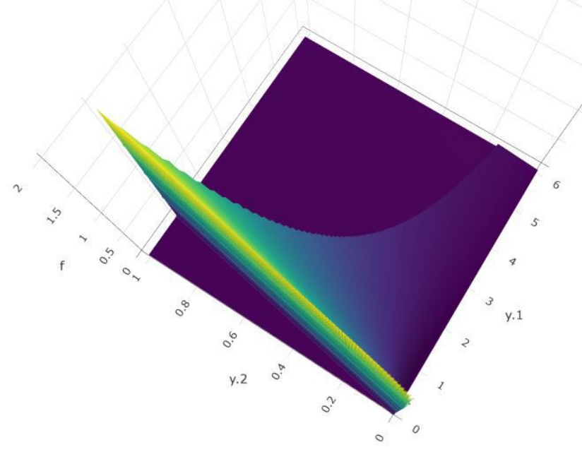
Figure 4: Support sets in Example 9. Left panel: bivariate support of (inside and boundary of green unit square), with and in red; right panel: bivariate support of (boundary and region between green curve and horizontal axis), with (half-open rectangle) in red.
Example 9 (DeGroot and
Schervish 2012, p. 183). In a departure from the previous notation in the paper, let have the following joint PDF:
(46)
and are clearly independent in this joint PDF, with marginal PDFs on for (the left panel of Figure 4 illustrates the support sets for ). Consider the interesting transformation under which ; intuitively and must be dependent, for example because they share the common multiplicative factor (interestingly, the correlation between and is about , when intuition might have suggested a positive association; the reason is the long right tail for large values of in Figure 5). It’s a matter of some tedium to demonstrate this in the usual way, because (a) you need to compute the Jacobian matrix of the inverse transformation to get the joint PDF of and then (b) you have to extract the marginals for the ; our method also requires some attention to detail but may arguably be less tedious, as follows. Considering the realized values and of and , respectively, a brief calculation reveals that the inverse transformation is given by . Solving the system of inequalities in the new coordinates yields the set in the right panel of Figure 4 (the oddly-shaped region on and below the green piecewise curve), which is the transformed image of the unit square in the left panel of that Figure; here and . Their Cartesian product (the half-open rectangle outlined in red in the right panel) is clearly unequal to , i.e., our Theorem 1 and Proposition 3 demonstrate dependence of and . We conclude this slightly strange example with a perspective plot (Figure 5) of the more-than-slightly-strange joint PDF in the coordinate system.
Figure 5: A perspective plot of the bivariate PDF in Example 9 (higher PDF values in yellow).
8 Discussion
The environment in which two real-valued random variables and are independent is replete with factorization: under independence, the joint CDF factors into the product of the marginal CDFs, and the same is true on the PMF and (with some care in stating the result) PDF scales. In this paper we add yet another scale with analogous behavior: if and are independent, the joint support set factors into the product of the marginal support sets. The contrapositive of this result offers a simple necessary condition for independence: if the joint support does not correctly factor, the random variables must be dependent. This will in some cases ease the burden of proof when exploring independence, as the examples in Section 7 illustrate. It has been an interesting journey, crucially involving simple ideas in measure theory and topology, to demonstrate this basic probabilistic finding.
Appendix
Here we present a proof sketch that supports our main finding at a high level of abstraction, based on suggestions from Terenin (2021, personal communication) and definitions and theorems from Kallenberg 2021, abbreviated in what follows; also see Williams 1991 for a deeply and highly usefully intuitive account of the fundamental measure theory and topology needed here. Familiarity with the following topics is assumed in this Appendix: measurable function, measurable space, probability space, product measure, product topology, and topological space.
Start with an arbitrary probability space , and consider
a measurable function that takes into a measurable space ; calls a random element in . By the definition of measurable functions, for any set we can speak meaningfully (a) of the set and (b) of the derived probabilities . As observes, the set function is a probability measure on , which may be termed the distribution of ; differs from ordinary usage in reserving the term random variable only for those situations in which .
To get two or more independent random elements up and running, establishes the following results.
6.
(Kallenberg (2021)) Let and be -finite measure spaces. Then there exists a unique (product) measure on such that
(47)
Remark 25. This result extends with no new ideas to -finite measure spaces for all finite integers .
7.
(Kallenberg (2021)) Let be random elements with distributions , respectively, in some measurable spaces . Then the are independent iff has distribution .
’s general definition of support is as follows.
13.
(Kallenberg (2021)) For any measure on a topological space , the support of is the set of points such that for every neighborhood of .
Remark 26. This matches the first result in Billingsley’s Lemma 2 in Section 3.3, when specialized to .
We can now state our basic result at this level of abstraction.
2.
(new) Let be random elements with distributions , respectively, in some measurable spaces , in which is equipped with the product topology. If the are independent, then the support of the product measure must factor:
(48)
Proof:
(sketch) The exact same proof as in Theorem 1 works here with the obvious necessary modifications:
(1)
Show that the two sets in equation (48) are equal by showing (a) that and (b) that ;
(2)
For (1)(a), pick an arbitrary point and build both a (Cartesian product) box and a (neighborhood) ball around such that the box contains the ball; use independence, ’s support definition and Fact from Proposition 1 to conclude that ; and
(3)
For (1)(b), pick an arbitrary point and again build both a (Cartesian product) box and a (neighborhood) ball around , but this time such that the ball contains the box; again use independence, ’s support definition and Fact from Proposition 1 to conclude that .
Acknowledgments
We’re grateful to John Kolassa, Alex Terenin, and David Williams for helpful references and comments. Membership on this list does not constitute agreement with the views presented here, nor are any of these people responsible for any errors that may remain.
References
Ash and
Doléans-Dade (2000)
Ash, R. and C. Doléans-Dade (2000).
Probability and Measure Theory (Second Edition).
London: Academic Press.
Billingsley (1995)
Billingsley, P. (1995).
Probability and Measure (Third Edition).
New York: Wiley.
Breiman (1992)
Breiman, L. (1992).
Probability.
Philadelphia: Society For Industrial and Applied Mathematics.
Cantor (1891)
Cantor, G. (1891).
Ueber eine elementare frage der mannigfaltigkeitslehre.
Jahresbericht der Deutschen Mathematiker-Vereinigung1,
75–78.
DeGroot and
Schervish (2012)
DeGroot, M. and M. Schervish (2012).
Probability and Statistics (Fourth Edition).
Boston: Addison-Wesley.
Dovgosheya et al. (2006)
Dovgosheya, O., O. Martio, V. Ryazanov, and M. Vuorinen (2006).
The Cantor function.
Expositiones Mathematicae24, 1–37.
Feller (1970)
Feller, W. (1970).
An Introduction to Probability Theory and Its Applications
(Volume II, Second Edition).
New York: Wiley.
Halmos (1974)
Halmos, P. (1974).
Measure Theory.
New York: Springer-Verlag.
Kallenberg (2021)
Kallenberg, O. (2021).
Foundations of Modern Probability (Third Edition).
Switzerland: Springer Nature.
Kolmogorov (1933)
Kolmogorov, A. (1933).
Grundbegriffe der Wahrscheinlichkeitsrechnung.
Ergebnisse der Mathematik und Ihrer Grenzgebiete. 1. Folge, 2.
Shiryaev (1996)
Shiryaev, A. (1996).
Probability (Second Edition).
New York: Springer-Verlag.
Williams (1991)
Williams, D. (1991).
Probability with Martingales.
Cambridge: University Press.